Massive Parallel Quantum Computer Simulator
Abstract
We describe portable software to simulate universal quantum computers on massive parallel computers. We illustrate the use of the simulation software by running various quantum algorithms on different computer architectures, such as a IBM BlueGene/L, a IBM Regatta p690+, a Hitachi SR11000/J1, a Cray X1E, a SGI Altix 3700 and clusters of PCs running Windows XP. We study the performance of the software by simulating quantum computers containing up to 36 qubits, using up to 4096 processors and up to 1 TB of memory. Our results demonstrate that the simulator exhibits nearly ideal scaling as a function of the number of processors and suggest that the simulation software described in this paper may also serve as benchmark for testing high-end parallel computers.
pacs:
03.67.Lx, 02.70.-cI Introduction
In this paper, we describe a Fortran 90 software package to simulate universal quantum computers NIEL00 . The software runs on various computer architectures, ranging from PCs to high-end (vector) parallel machines. The simulator can perform all the quantum operations that are necessary for universal quantum computation. The maximum number of qubits is set by the memory of the machine on which the code runs. We present simulation results for quantum computers containing up to 36 qubits. In view of the fact that the simulation of quantum systems, such as quantum computers, requires computational resources that grow exponentially with the system size, this represents a significant advance beyond the state of the art, which is currently around 32 qubits FRAU05 . An overview of quantum computer simulator software is given in Ref. RAED05 .
The main focus of the present work is on the design of portable, efficient parallel simulation code for a universal quantum computer. A subsequent paper TRIE06 will explore optimization techniques to further improve the performance of the parallel code. In principle, because of this “universality”, this code for the ideal quantum computer can also be used to simulate physical systems, such as quantum spin models or models for physical realizations of quantum computers, by writing the time evolution of the physical system as a sequence of elementary quantum gate operations NIEL00 . However, this approach is bound to be computationally inefficient for all but nontrivial physical systems. Instead, it is much more effective to allow for additional unitary transformations that implement operations such as the time evolution under a Heisenberg Hamiltonian in an optimal manner RAED00 ; QCEDOWNLOAD ; RAED02 ; RAED05 . Such an extension, which does not affect the intrinsic performance of the code, will be dealt with in a future publication.
The paper is organized as follows. In Section II, we briefly recall some basic elements of quantum computation. In Section III, we present a scheme to parallelize the software to simulate a quantum computer on a massive parallel computer. We employ the standard Message Passing Interface (MPI) MPI to implement this scheme. Section IV describes the main features of the simulator software. In Section V, we discuss a few nontrivial quantum algorithms, such as an adder of two to five registers of qubits and Shor’s factoring algorithm, that are used to validate and benchmark the simulation software. Section VI presents our benchmark results of running the quantum algorithms on various parallel computers. A discussion is given in Section VII.
II Quantum Computation
For convenience of the reader, to make the paper self-contained and to explain the terminology, we summarize some basic aspects of quantum computation.
II.1 Quantum computer terminology
The state of a qubit, the elementary storage unit of a quantum computer, is described by a two-dimensional vector of Euclidean length one:
| (1) |
where and denote two orthogonal basis vectors of the two-dimensional vector space and and are complex numbers such that . The result of inquiring about the state of a single qubit, that is the outcome of a measurement, is either 0 or 1. The frequency of obtaining 0 (1) can be estimated by repeated measurement of the same state of the qubit and is given by () SCHI68 ; BAYM74 ; BALL03 .
The internal state of a quantum computer with qubits is described by a vector, also called the state vector, in a dimensional space NIEL00 . Adopting the convention of quantum computation literature NIEL00 , the state of an -qubit quantum computer is represented by
| (2) | |||||
where in the last line of Eq. (2), the binary representation of the integers was used to denote and . We normalize the state vector, that is , by rescaling the complex-valued amplitudes according to
| (3) |
Note that in this notation it is convenient to number the qubits from 0 to , that is qubit 0 corresponds to the least significant bit of the integer index that runs from zero to .
A quantum algorithm is a sequence of unitary operations on the vector . It has been shown that an arbitrary unitary operation can be written as a sequence of single qubit operations and the CNOT operation on two qubits DIVI95a ; NIEL00 . Therefore, single-qubit operations and the CNOT operation are sufficient to construct a universal quantum computer NIEL00 . We call these operations elementary unitary transformations. According to quantum theory, after executing a quantum algorithm, the probability for observing the quantum computer in one of its states is given by the square of the absolute value of the corresponding element of the state vector.
In the quantum computation literature, the convention is to count each elementary, unitary transformation as one operation on a quantum computer NIEL00 . However, carrying out a unitary operation on a conventional computer requires more than one arithmetic operation and it is customary to determine the performance of an algorithm by counting the number of arithmetic operations. Although the difference between these two ways of expressing the performance of an algorithm should be clear from the context, the reader should keep this difference in mind.
II.2 Single-qubit operations
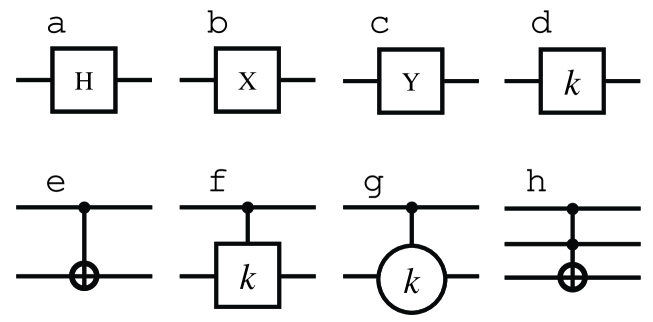
Single-qubit operations that are often used in quantum computation are the Hadamard operation and rotations and of the state vector by about the and -axis of the spin-1/2 operator , representing the qubit. The Hadamard operation is defined by NIEL00
| (4) | |||||
the operation by
| (5) | |||||
and the operation by
| (6) | |||||
The phase shift operation is defined by
| (7) | |||||
changes the phase of the amplitude of the component of the state vector only. Quantum algorithms are often represented by quantum networks, diagrams that show the order of the operations performed on the qubits. The graphical symbols of , , , and are shown in Fig. 1. The inverse and transpose of a unitary operation are denoted by and , respectively.
II.3 Two-qubit operations: CNOT and controlled phase shift
Computation requires some form of communication between the qubits. Any form of communication between qubits can be reduced to a combination of single-qubit operations and the CNOT operation, a two-qubit operation DIVI95a ; NIEL00 . By definition, the CNOT gate flips the target qubit if the control qubit is in the state NIEL00 . If we take qubit zero (that is the least significant bit in the binary notation of an integer) as the control qubit and qubit one as the target qubit then we have
| (8) | |||||
The graphical symbol of the CNOT operation is shown in Fig. 1e. The dot (cross) denotes the control (target) qubit.
Another frequently used operation is the controlled phase shift. The controlled phase shift operation with control qubit 0 and target qubit 1 is defined by
| (9) | |||||
Graphically, the controlled phase shift is represented by a vertical line connecting a dot (control qubit) and a box denoting a single qubit phase shift by (see Fig. 1f).
The CNOT operation is a special case of the controlled unitary transformation . If qubit zero is the control qubit and qubit one is the target qubit then
| (10) | |||||
The graphical symbol of the controlled operation, , is a vertical line connecting a dot and a circle containing the value (see Fig. 1g).
II.4 Three-qubit operation: Toffoli gate
The Toffoli gate is a generalization of the CNOT gate in the sense that it has two control qubits and one target qubit BARE95 ; NIEL00 . The target qubit flips if and only if the two control qubits are set. If we take qubit zero and qubit one as the control qubits and qubit two as the target qubit then we have
| (11) | |||||
Symbolically the Toffoli gate is represented by a vertical line connecting two dots (control qubits) and one cross (target qubit), as shown in Fig. 1h.
III Parallelization
III.1 General computational aspects
Computer memory and CPU time put limitations on the size of the quantum computer that can be simulated on a conventional digital computer. The required CPU time is mainly determined by the number of operations to be performed on the qubits. The CPU time does not put a hard limit on the simulation. However, the memory of the computer does. According to Eq. (2), the state of a -qubit quantum computer is represented by a complex-valued vector of length . In view of the potentially large number of arithmetic operations, it is advisable to use 13 - 15 digit floating-point arithmetic (corresponding to 8 bytes for a real number). Thus, to represent a state of the quantum system of qubits in a conventional, digital computer, we need at least bytes. Hence, the amount of memory that is required to simulate a quantum computer with qubits increases exponentially with the number of qubits . For example, for () we need at least 256 MB (1TB) of memory to store a single arbitrary state .
As seen in Section II, operations on the state vector result in a transformation of the amplitudes of the basis states in . More specifically, let us denote
| (12) |
and
| (13) | |||||
We first consider the single-qubit operations on qubit that transform in . From Eq. (4), it follows that the Hadamard operation on qubit , , transforms the amplitudes according to
| (14) |
where we use the asterisk to indicate that the bits on the corresponding positions are the same. From Eq. (5), it follows that for operating on the elements of are obtained by
| (15) |
In the case of , it follows from Eq. (6) that
| (16) |
From Eq. (7) it follows that we obtain by leaving the amplitudes, for which the th bit of their index is zero, unchanged and by multiplying the amplitudes, for which the th bit of their index is one, with the phase factor . Hence we have,
| (17) |
In summary, performing an operation on qubit requires in general an update of elements of . The single-qubit phase shift operation forms an exception and requires an update of single amplitudes only. Note that all these operations can be done in place, that is, without using another vector of length .
We now consider two-qubit operations , with . For the CNOT operation , where qubit is the control qubit and qubit is the target qubit, amplitudes for which bit of their index is one and bit of their index is zero need to be swapped with amplitudes for which bits and of their index are one (see Eq. (8)). We have
| (18) |
For the controlled- operation , it follows from Eq. (10) that the amplitudes change according to the rules
| (19) |
Thus, performing two-qubit operations such as the CNOT and the controlled- amount to update amplitudes.
For the Toffoli gate (), where qubits and are the control qubits and qubit is the target qubit, only elements of need to be updated, as can be seen from Eq. (11). The update rules read
| (20) |
and the other amplitudes remain unchanged.
All the qubit operations discussed here can be carried out in floating-point operations (here and in the sequel, if we count operations on a conventional computer, we make no distiction between operations such as add, multiply, or get from and put to memory). The qubit operations described earlier suffice to implement any unitary transformation on the state vector. As a matter of fact, the simple rules described are all that we need to simulate a universal quantum computer on a conventional computer.
The fact that both the amount of memory and arithmetic operations increase exponentially with the number of qubits is the major bottleneck for simulating quantum computers (or quantum systems in general) on a conventional computer. However, in contrast to the CPU time, the total amount of memory that is available on a computer puts a hard limit on the simulations that can be performed. From the user’s perspective, the memory on a computer can be shared or distributed. On a shared memory computer, the state of the quantum computer can be completely stored in the memory and all processors can access the entire memory. On a distributed memory machine, the elements of are physically distributed over different nodes and each processor has direct access to its own local memory only. In the latter case, some extra programming is required to perform the communication between the processors. We use the standard Message Passing Interface (MPI) to perform the data communication MPI . We assume that the reader has some basic knowledge of MPI programming MPI .
III.2 Implementation
Each MPI process has a rank and a local memory. We assume that the local memory can store the amplitudes of the basis states of qubits. Hence, to simulate a -qubit quantum computer we need MPI processes. From Eq. (2), it is clear that the amplitudes where for , can be stored at the local memory address of the MPI process with rank . In binary notation the local memory address and the rank of the processor reads and , respectively. Recall that the qubits are numbered from 0 to , that is qubit 0 corresponds to the least significant bit of the integer index, running from zero to , of the amplitude. An example for and is shown in the first four columns of Table 1. The MPI processes are labeled with their ranks running from to . The memory addresses are also running from to for this example.
| 00 | 01 | 10 | 11 | 00 | 01 | 10 | 11 | 00 | 01 | 10 | 11 | |
| 00 | a(0000) | a(0100) | a(1000) | a(1100) | a(0000) | a(0001) | a(1000) | a(1001) | a(0000) | a(0001) | a(0100) | a(0101) |
| 01 | a(0001) | a(0101) | a(1001) | a(1101) | a(0100) | a(0101) | a(1100) | a(1101) | a(1000) | a(1001) | a(1100) | a(1101) |
| 10 | a(0010) | a(0110) | a(1010) | a(1110) | a(0010) | a(0011) | a(1010) | a(1011) | a(0010) | a(0011) | a(0110) | a(0111) |
| 11 | a(0011) | a(0111) | a(1011) | a(1111) | a(0110) | a(0111) | a(1110) | a(1111) | a(1010) | a(1011) | a(1110) | a(1111) |
As can be seen from Eqs. (14)-(17), performing an operation on qubit requires in general an update of elements of . A qubit for which we call a “local” qubit. In the example shown in the first four columns of Table 1 qubits 0 and 1 are local qubits. Updating the amplitudes is easy if the qubit is local because this requires no communication between the MPI processes.
Similarly, if we call qubit a “nonlocal” qubit. An operation on qubit requires communication between the MPI processes. In the example shown in the first four columns of Table 1, qubits 2 and 3 are nonlocal. Note that the nonlocal qubits form the binary representation of the rank of the corresponding MPI process and that the local qubits form the binary representation of the memory address. An obvious way of communication would be for pairs of MPI processes to first interchange one half of their data. Then, the operations on the amplitudes can be performed as if the qubit was local. Finally, the MPI processes need again to interchange the (modified) data. A clear drawback of this method is that half of the amplitudes needs to be interchanged twice for every single-qubit operation on qubit for which .
In order to reduce the amount of communication between the MPI processes we use a different method to handle the operation on nonlocal qubits. We introduce a permutation of the qubits. We denote the permutation by a matrix with two rows and columns. The first row contains integer numbers ordered from to 0. These numbers correspond to the position of the bits in the index of the amplitude. The second row also contains integer numbers ranging from to 0 but they are not necessarily ordered. These numbers refer to the qubits. Local qubit corresponds to bit of the index of the amplitude and nonlocal qubit corresponds to bit of the index of the amplitude. After applying the permutation the amplitudes () are stored at the address of the local memory assigned to the MPI process with rank . In binary notation we have and . Note that after applying the permutation , the nonlocal qubits still form the binary representation of the rank of the corresponding MPI process. Similarly, the local qubits still form the binary representation of the address.
Logically, to make a nonlocal qubit local, all we have to do is to select a permutation that interchanges a local qubit, say , and the nonlocal qubit and leaves the other qubits in place. Clearly, it is always easy to find such a permutation. We now consider what it actually means for the parallel machine to perform an interchange of a local and nonlocal qubit. A simple reshuffling of the corresponding amplitudes would work but is not very efficient: We would like to minimize the amount of interprocess communication.
In terms of data transfer between MPI processes, a permutation that interchanges local qubit and nonlocal qubit , swaps the amplitudes with addresses
| of MPI process with rank | |||||
| and | |||||
| of MPI process with rank | (21) |
where we use the asterisk to indicate that the bits on the corresponding position are the same. Hence, in this operation, only half of the amplitudes in the memory of an MPI process are swapped against half of the amplitudes in the memory of another MPI process. After this swap operation, the previously nonlocal qubit has become local, and we can carry out the operations on this qubit in exactly the same way as we did for the originally local qubits, that is fully parallel. Using this scheme we don’t need to send the modified amplitudes back to the MPI processes from which they originate as the permutation keeps track of the memory adresses of the amplitudes.
An example of this process of swapping data is shown in Table 1, for , . The permutations that have been applied are shown on the top row. The four columns below show the original content of the local memories. In this example, qubits 0 and 1 are local and qubits 2 and 3 are nonlocal. Hence, operations on qubit 0 or 1 can be performed in parallel by each MPI process. However, operations on qubit 2 and 3 require communication between the MPI processes. Let us now assume that we want to carry out an operation on qubit 2. According to our scheme, this requires that the pairs of amplitudes and reside in the same local memory. Conceptually, this can be accomplished by rearranging the amplitudes over the local memories according to the permutation (see Table 1) whereas the actual data exchange is carried out according to Eq. (21).
Now qubits 2 and 1 are local and qubits 0 and 3 are nonlocal. Assume that we now want to operate on qubit 3 which is currently nonlocal. Then, we may interchange, for example, local qubit 2 with the nonlocal qubit 3. This can be accomplished by applying the permutation (see Table 1) and data exchange rule Eq. (21). At this point, qubits 3 and 1 are local and qubits 0 and 2 are nonlocal.
To summarize: A single-qubit operation on a nonlocal qubit consists of a local-nonlocal data exchange defined by Eq. (21), followed by the actual unitary operation. By construction, there is no interprocess communication during and after the latter. If the qubit is local, we simply skip the step of exchanging data. From Eq. (17), it is clear that the single-qubit phase-shift operation never requires communication between MPI processes. Thus, for this particular operation there is additional room for optimization. In our present simulation code, we have choosen not to optimize gate operations on this level. Optimization of parallel code for specific gates will be dealt with in depth in a subsequent publication TRIE06 .
| 00 | 01 | 10 | 11 | 00 | 01 | 10 | 11 | |
| 00 | a(0000) | a(0100) | a(1000) | a(1100) | a(0000) | a(0001) | a(0010) | a(0011) |
| 01 | a(0001) | a(0101) | a(1001) | a(1101) | a(0100) | a(0101) | a(0110) | a(0111) |
| 10 | a(0010) | a(0110) | a(1010) | a(1110) | a(1000) | a(1001) | a(1010) | a(1011) |
| 11 | a(0011) | a(0111) | a(1011) | a(1111) | a(1100) | a(1101) | a(1110) | a(1111) |
Extending the single-qubit scheme to two and three-qubit operations is conceptually straigthforward but the rules to determine which processes have to exchange data become more complicated. From Eqs. (18) and (19), it follows that a two-qubit operation involves an update of elements of . If these elements are located in the same local memory, that is if both qubits are local, no communication between the MPI processes is required and the operation can be performed independently by all the MPI processes. However, if one of the qubits is nonlocal, some communication is necessary. If only one qubit is nonlocal, we can use the same procedure as described above to interchange the qubit for a local one. If both qubits are nonlocal, we can also use the same procedure, but twice. For each qubit interchange, half of the amplitudes in the memory of a MPI process is swapped against half of the amplitudes in the memory of another MPI process. Hence, this scheme results in a full memory swap. However, this amount of communication can be reduced by exchanging two nonlocal qubits and two local qubits simultaneously. We illustrate this by the example for the case , , shown in Table 2. The four columns below show the original content of the local memory. In this example, qubits 0 and 1 are local and qubits 2 and 3 are nonlocal. Hence, two-qubit operations on qubit 0 and 1 can be performed independently by each MPI process. However, all other two-qubit operations require communication between the MPI processes.
Let us now assume that we want to do a two-qubit operation on qubits 2 and 3. Permutation interchanges nonlocal qubits 2 and 3 with local qubits 0 and 1, respectively. From Table 2 we see that each MPI process has to communicate with three other processes. For example, MPI process keeps the amplitude in address , interchanges its amplitude in address with the amplitude in address of MPI process , interchanges its amplitude in address with the amplitude in address of MPI process , and interchanges its amplitude in address with the amplitude in address of MPI process .
In general, for a two-qubit interchange, the MPI processes communicate in groups of four (in the example of Table 2 there is only one group of four). Each MPI process keeps one quarter of the amplitudes in its local memory and interchanges the other three quarters of amplitudes with amplitudes in the local memories of the other MPI processes in the group. Swapping of the amplitudes can be accomplished by applying the permutation of the qubits so that the MPI processes interchange local qubits , for nonlocal qubits , . Local qubit corresponds to bit of the index of the amplitude and nonlocal qubit corresponds to bit of the index of the amplitude, where . Adopting the convention that and , interchanging local qubits , and nonlocal qubits , amounts to swapping the amplitudes with local memory addresses
| of MPI process with rank | |||||
| and | |||||
| of MPI process with rank | (22) |
| of MPI process with rank | |||||
| and | |||||
| of MPI process with rank | (23) |
| of MPI process with rank | |||||
| and | |||||
| of MPI process with rank | (24) |
| of MPI process with rank | |||||
| and | |||||
| of MPI process with rank | (25) |
| of MPI process with rank | |||||
| and | |||||
| of MPI process with rank | (26) |
| of MPI process with rank | |||||
| and | |||||
| of MPI process with rank | (27) |
As before, the asterisks in Eqs. (22)-(27) indicate that the bits on the corresponding position are the same. As in the case of the single-qubit operations, particular two-qubit operations (such as the controlled phase shift) allow for additional optimization, but we have choosen not to do so because we wanted to implement all two-qubit operations in the same manner.
The algorithm to interchange a pair of local qubits with a pair of nonlocal qubits (see Eqs. (22)-(27)) can be generalized to swap as many local qubits with nonlocal qubits, with the restriction that the number of qubits to be swapped cannot exceed the number of local or nonlocal qubits. Exchanging pairs of local and nonlocal qubits simultaneously requires each MPI process to send amplitudes to another MPI process. Sequentially exchanging the pairs amounts to sending amplitudes to another process. Thus, exchanging pairs of local and nonlocal qubits simultaneously involves less communication. However, the more qubits we swap simultaneously, the larger becomes the group of MPI processes that communicate with each other. If this number becomes too big the computer might hang in network collisions. So, in practice there is a limit to the choice of . In our implemention of the algorithm, is an input variable. For each MPI process, we first compute the ranks of the other MPI processes with which the MPI process has to communicate. We do this on the basis of the pairs of local and nonlocal qubits that need to be swapped. Before exchanging data between the MPI processes belonging to one group, we fill a buffer for each MPI process of the group. The buffer contains all amplitudes that need to be send from one MPI process to the other MPI processes of the group. In order to reduce the memory allocation for the buffers, an essential requirement for simulating quantum computers with a large number of qubits , we split the MPI send instruction in a fixed (user controlled), smaller number of send instructions.
IV Simulator
We have implemented the algorithm described in Section III in Fortran 90. The computer code contains all quantum operations that are necessary for universal quantum computation and runs on machines with distributed and/or shared memory. Standard MPI is used for interprocess communication. Optionally, OpenMP can be used for parallel processing within each MPI process. This computer code forms the engine of the parallel quantum computer simulator. It compiles (without modifications) and runs on various computer architectures, ranging from PCs to high-end (vector) parallel machines. The number of qubits in the computer codes is limited to 62, but in practice the maximum number of qubits is set by the memory of the machine on which the code runs.
The simulator takes as input the description of a quantum network in terms of pseudocode (a text-formatted file). Quantum networks are drawn by making use of a graphical user interface. For this purpose, we developed Quantum Computer Circuit Editor (QCCE), a Microsoft Windows application. QCCE contains graphical symbols for each of the qubit operations described in Section II and for the quantum Fourier transform. Examples of quantum networks drawn by QCCE are shown in Fig. 2 and Fig. 3. QCCE also contains an interpreter that takes the quantum network as input and generates a text-formatted file that contains pseudocode describing all operations to be performed on the qubits, including the swap operations described in Section III.2. An example of the pseudocode is given in appendix A. Since drawing a quantum network for a large quantum computer can be quite cumbersome, it is often more efficient to write a dedicated program that generates the pseudocode language directly. Since the quantum computer simulator software is a standalone application that takes ASCII files as input, any software package (such as http://www.phys.cs.is.nagoya-u.ac.jp/~watanabe/qcad/index.html) that can draw quantum networks may be used, as long as it generates the input files (including the swap operations) in the format that the simulator can understand.
| SGI Altix 3700 | IBM Regatta p690+ | IBM Blue Gene/L | Hitachi SR11000/J1 | Cray X1E | |
| Location | SARA | FZ-J | RuG | ISSP | CRAY Inc. |
| Memory | 832 GB | 5.2 TB | 3.1 TB | 2.8 TB | 512 GB |
| # CPUs | 416 | 1312 | 12288 | 2048 | 128 |
| CPU type | Intel Itanium 2 | Power 4+ | Power PC 970 | POWER5 | 64-bit Cray X1E MSP |
| CPU clock | 1.3 GHz | 1.7 GHz | 0.7 GHz | 1.9 GHz | 1.13 GHz |
V Simulation results
In this section we present and discuss the results of running the massive parallel quantum computer simulator on various parallel computers.
The computers on which we perform the simulations and their characteristics are listed in Table 3. On all computers we have tested pure OpenMP, pure MPI and combined MPI/OpenMP code. In practice it turns out that the OpenMP code is up to a factor of two slower than the pure MPI code. As a consequence, also the MPI/OpenMP code is slower than the pure MPI code. A detailed study of the (dis)advantages of this hybrid approach in the case of optimized parallel code for specific gates will be presented in a future publication TRIE06 . In what follows we only present the results of the pure MPI code. Because of the special architecture of the Cray X1E processors (Cray Multistreaming Processors (MSPs) with various vector pipes per MSP), some CRAY specific directives have been added to the code.
A rather simple algorithm to test the scaling properties of the simulation software with the number of qubits is to perform a Hadamard operation on each qubit of a -qubit quantum computer. However, simulating gates for single-, two- and three-qubit operations only is not sufficient to test the correctness of quantum computer simulation software and to compare the performance of various massive parallel computers. Hence, for this purpose, we consider some more sophisticated quantum algorithms. A first nontrivial example is the qubit adder that adds the content of several qubit registers. This quantum algorithm is built up from several quantum operations, including a quantum Fourier transform, and has the advantage that it is very easy to check the correctness of the simulation result.
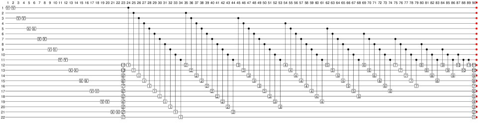
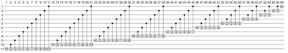
Figure 2 shows the quantum network to add the content of two eleven-qubit registers. Note that here the qubits are numbered starting from one. We use a similar modular structure as was used for adding the content of three four-qubit registers BETT02 . The basic idea of the algorithm is to use the Quantum Fourier Transform (QFT) to first transfer the information in one register to the phase factors of the amplitudes, then use controlled phase shifts to add the information from the other registers, and finally QFT back to the original representation. These quantum networks perform addition modulo two to the power of the number of qubits in the register on which the QFT is being applied.
Originally all qubits are in the state . The single-qubit operations , , and are used to put numbers (in binary notation) in the registers. Note that all these operations bring a qubit in the state . Hence, in principle we could use only one of these operations to put numbers in the registers. However, in order to test the various single-qubit operations we used the four different operations. In the example shown in Fig. 2 the first register (qubits 1 to 11) contains the number 1365 and the second register (qubits 12 to 22) the number 682. We perform a QFT on the second register to transfer the information in the second register to the phase factors of the amplitudes. The full quantum network for a QFT on eleven qubits is shown in Fig. 3. After applying the QFT to the second register, we use controlled phase shifts to add the information from the first register to the content of the second one. Finally we QFT back to the original representation.
As another nontrivial test we implement Shor’s algorithm on a quantum computer containing up to 36 qubits. Briefly, Shor’s algorithm finds the prime factors and of a composite integer by determining the period of the function for Here, should be coprime (greatest common divisor of and is 1) to (otherwise, since , or , so we already guessed the solution). Let denote the period of , that is . If the chosen value of yields an odd period , we repeat the algorithm with another choice for , until we find an that is even. Once we have found an even period , we compute . If , then we find the factors of by calculating the greatest common divisors of and .
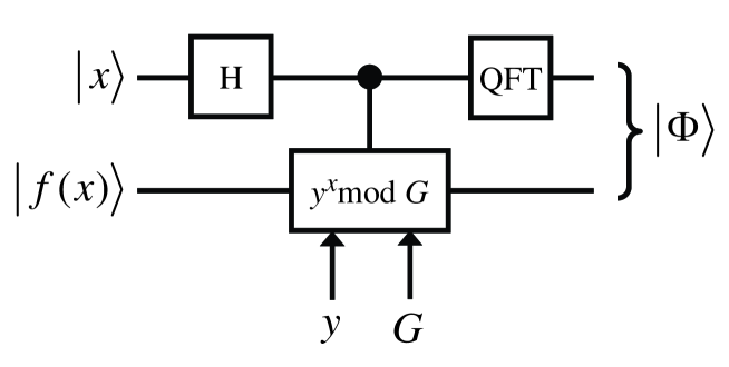
On an ideal quantum computer, this algorithm can be carried out with a number of unitary operations that increases as a polynomial, not as the exponential, of the number of qubits required to store the number . The schematic diagram of Shor’s algorithm is shown in Fig. 4. The quantum computer has qubits. There are two qubit registers: A -register with qubits to hold the values of and a -register with qubits to hold the values of . What is the largest number we can factorize on a quantum computer with qubits? If we write the number in its binary representation , where , then it is clearly seen that . For Shor’s algorithm to work properly, that is to find the correct period of , the number of qubits in the -register should satisfy SHOR99
| (28) |
Writing , where , it follows from Eq. (28) that . Omitting numbers that can be written as a power of two (which are trivial to factorize), the smallest value for (and hence the largest value for ) is given by . Hence, . Since either or , it follows that the maximum number of qubits that can be reserved for the -register is give by . For example, on a 36-qubit quantum computer is the largest integer that can be factorized by Shor’s algorithm.
The initial state of the machine is . After applying Hadamard operations to all qubits of the -register we have
| (29) |
where and denote the state of the and -register, respectively. Then, we compute for each value . This is implemented as a conditional operation, as indicated by the middle box in Fig. 4. After the second step, the quantum computer is in the state
| (30) |
The period of can now be determined by applying a Fourier transformation, not to but to , as indicated in Fig. 4. To see how this step works, we use the periodicity of to rewrite Eq. (30) as
| (31) |
Using the Fourier representation of we obtain
| (32) | |||||
where denotes the largest integer such that . The probability to observe the quantum computer in the state reads
| (33) |
The function is strongly peaked for all . The probability to observe the machine in the state for which is EKER96 . Given the observed state , we can find because the condition Eq. (28) guarantees that there exists exactly one function that satisfies SHOR99
| (34) |
The fraction (with ) can be found effectively by computing the convergents of the continued fraction representation of HARD00 ; SHOR99 ; EKER96 ; NIEL00 . From Eq. (33) we can easily compute the expectation values of the qubits of the -register. Let for , then
| (35) | |||||
where denotes the th bit of . The quantum computer simulator should reproduce the values of all , for , otherwise there is definitely something wrong in the simulation. On the other hand, agreement is not a guarantee that the simulator is free of errors. Obviously, for a qubit simulation, storing the final state for further analysis requires a lot ( 1TB) of disk space. To alleviate this problem, we have added to the simulator a procedure that takes the final state as input and generates a user-specified number of basis states with probability . This procedure is also fully parallel and uses all available MPI processes.
In Table 4 we show the results of running Shor’s algorithm on the massive parallel computer simulator. The example for qubits was run on an IBM Thinkpad T43P. The two examples for qubits were both run on the SGI Altix 3700 and on the IBM Regatta p690+. The two examples for are both run on the IBM Regatta p690+ and on the IBM Blue Gene/L. All the tests desribed in this section confirm that the simulator is producing correct results.
VI Benchmark results


The quantum algorithms that we use for benchmarking the simulator software are the Hadamard operation performed on each qubit, qubit adders to add the content of three 11-qubit registers, two 17-qubit registers, five 7-qubit registers and three 12-qubit registers. Tables 5-9 of appendix B summarize the results on the various machines. In order to compare the performance of the different machines we use the data from Tables 5-9 and plot them in Figs. 5-7. Figure 5 depicts the elapsed time divided by the CPU time and multiplied by the number of MPI processes as a function of the number of qubits . All data listed in Tables 5-9 is processed. In the ideal case, we expect that , independent of . As can be seen from Fig. 5, on most machines we observe scaling properties that are very close to ideal. Deviations from the ideal behavior, if there are any, are relatively small. The IBM Regatta p690+ and the Cray X1E show the largest deviations.
In Fig. 6 we show the CPU time for a Hadamard operation carried out on qubit of a quantum computer with qubits. In this case the CPU time is measured per gate and does not include the time for measuring the qubit. Recall that we number the qubits starting from zero, so that . We only show results for the IBM Regatta p690+ (diamonds), IBM Blue Gene/L (flipped triangles) and the Hitachi SR11000/J1 (circles). The number of MPI processes on the IBM Regatta p690+, the IBM Blue Gene/L and the Hitachi SR11000/J1 are , and , respectively. Hence, on the IBM Regatta p690+ and the Hitachi SR11000/J1 qubits are local and on the IBM Blue Gene/L qubits are local. In all cases, the CPU time for carried out on a nonlocal qubit is equal to the CPU time for the Hadamard gate performed on qubit zero, because according to the algorithm described in Section III.2, we interchange the nonlocal qubit with the local qubit zero. On the IBM Regatta p690+, the CPU time to carry out on a local qubit can differ by a factor of three depending on the qubit number . This is a result of how the local memory addresses are accessed and is thus due to the architecture of the machine. Techniques to speed up the memory access will be discussed in a future application TRIE06 . On the IBM Blue Gene/L and on the Hitachi SR11000/J1 we only see a relatively small increase in CPU time if we operate on qubits with inreasing number . The difference in behavior between the IBM Regatta p690+ and the two other machines is also reflected in Fig. 5, although there it is much less clear. Figure 6 clearly shows that the Hitachi SR11000/J1 is significantly faster than the IBM Regatta p690+ and the IBM Blue Gene/L.
Figure 7 shows as a function of , being the number of quantum operations (not including swap commands). All data listed in Tables 5-9 is processed. On all machines, the number of MPI processes , except on the IBM Blue Gene/L, . Therefore, for a program that parallelizes 100% we expect that , where is a constant. Hence, in the ideal case should be equal to . From Fig. 7 it can be seen that for all machines, is slightly increasing as a function of . The deviation from the ideal performance is due to the communication between various MPI processes. The corresponding increase in CPU time seems to be the largest for the IBM Regatta p690+ and the Cray X1E. However, the overall scaling properties of the simulation software are extremely good. For comparison we depict the line, given by , in Fig. 7. This line expresses the expected behavior of as a function of on a non-parallel computer, that is a computer for which . Clearly, with the available hardware and the present simulation software, it is possible to beat the exponential growth of the simulation problem by simply increasing the memory and the number of CPUs by a factor of two for each qubit added, at least up to 36 qubits.
From Tables 5-9 it is clear that from the point of view of the user, that is in terms of elapsed time, the IBM Blue Gene/L is the fastest computer. If we make a comparison based on the CPU time then the Cray X1E is the fastest machine, followed by the Hitachi SR11000/J1. We emphasize that, except for the Cray X1E, we have used the same source code on all machines, that is we did not make an effort to adapt the code for a particular machine.
Out of curiosity and to demonstrate the portability of the parallel simulation code, we also test the software on a cluster of three IBM Thinkpad T43P notebooks and one IBM Think Centre A50P PC, using MPICH2 under Windows XP. Communication between the machines is handled by a 100 Mbit Ethernet US Robotics router. In Table 10 we show the performance results for carrying out a Hadamard operation on each qubit. Explicit measurement of the time spent for communication between the machines shows that for the example with qubits, about half of and is spent on network communication.
VII Discussion
The parallel quantum computer simulator presented in this paper is an application that shows nearly perfect scaling with the number of CPUs and problem size. It is a demanding application in that it can use a significant part of the available memory and CPUs and can put a heavy burden on the communication network. Therefore, this simulator may find application as a new type of benchmark to assess the computational power of the new generation of high-end computer systems.
Acknowledgements.
Support from the “Nederlandse Stichting Nationale Computer Faciliteiten (NCF)” is gratefully acknowledged. We thank Gyan Bhanot (IBM Yorktown) for helping us with porting the code to the IBM BlueGene/L, ASTRON (NL) for providing access to the IBM BlueGene/L and Arnold Meijsters (RuG) for helping us with running the simulations on the IBM BlueGene/L. We are grateful to J. Thorbecke (Cray) for performing the benchmarks on the Cray X1E. We thank W. Frings at FZJ for fruitful discussions on hardware specifics of the IBM p690+. This work is partially supported by the Japanese Ministry of Internal Affairs and Communications (Soumu-sho). Finally, we thank the Supercomputer Center, Institute for Solid State Physics, University of Tokyo for the facilities and the use of Hitachi SR11000/J1.Appendix A Quantum Computer Circuit Editor (QCCE)
In this appendix we discuss the text-formatted file, generated by QCCE, that is used as input for the simulator if it has to simulate a Hadamard operation performed on each qubit of a 32-qubit quantum computer. Lines starting with “ ! ” or “ # ” are considered as comments. We use these symbols to add comments to the following text generated by QCCE:
QUBITS 32                         ! The command QUBITS sets the size of the quantum computer
INITIAL STATE 0                   ! The initial state of the quantum computer is set to |0...0>
MPIPROCESSES 32                   ! Number of MPI processes is set to 32
                                  ! (not used by the OpenMP code)
H 0                               ! Hadamard operation on qubit 0
.                                 ! These lines are omitted here but contain commands for
.                                 ! Hadamard operations carried out on qubits 1-25
.
H 26                              ! Hadamard operation on qubit 26
SWAP 1 0 27                       ! Command to swap 1 pair of qubits: qubits 0 and 27
H 27                              ! Hadamard operation on qubit 27
SWAP 1 27 28                      ! Command to swap qubits 27 and 28
H 28                              ! Hadamard operation on qubit 28
SWAP 1 28 29                      ! Command to swap qubits 28 and 29
H 29                              ! Hadamard operation on qubit 29
SWAP 1 29 30                      ! Command to swap qubits 29 and 30
H 30                              ! Hadamard operation on qubit 30
SWAP 1 30 31                      ! Command to swap qubits 30 and 31
H 31                              ! Hadamard operation on qubit 31
BEGIN MEASUREMENT
DO MEASUREMENT 1 2 3 4 5 6 7 8 9 10 11 12 13 14 15 16 17 18 19 20 21 22 23 24 25 26 31
                                  ! Measurement operation on the listed qubits
SWAP 5 31 1 2 3 4 0 27 28 29 30   ! Command to swap 5 pairs of qubits: (31,0), (1,27), (2,28),
                                  ! (3,29), and (4,30)
DO MEASUREMENT 0 27 28 29 30      ! Measurement operation on the listed qubits
END MEASUREMENT
As can be seen from the example, the general format of a command consists of a keyword followed by some values. Note that the swap command is not the same as the quantum swap operation. The swap command carries out the qubit interchange described in Section III.2.
Appendix B Simulation results
| Memory [GB] | [s] | [s] | Quantum algorithm | |||
|---|---|---|---|---|---|---|
| 27 | 1 | 2 | 27 | 144 | 142 | H |
| 28 | 2 | 4 | 28 | 159 | 304 | H |
| 29 | 4 | 8 | 29 | 156 | 646 | H |
| 30 | 8 | 16 | 30 | 202 | 1510 | H |
| 31 | 16 | 32 | 31 | 305 | 4040 | H |
| 32 | 32 | 64 | 32 | 453 | 13200 | H |
| 33 | 64 | 128 | 33 | 492 | 28600 | H |
| 34 | 128 | 256 | 34 | 526 | 61500 | H |
| 33 | 64 | 128 | 286 | 2568 | 157000 | 3-11QBA: 292+585+1170 |
| 34 | 128 | 256 | 493 | 4019 | 496000 | 2-17QBA: 26214+104857 |
| 35 | 256 | 512 | 194 | 2374 | 635000 | 5-7QBA: 7+9+19+35+65 |
| 36 | 512 | 1024 | 342 | 4095 | 1960000 | 3-12QBA: 781+1054+3296 |
| Memory [GB] | [s] | [s] | Quantum algorithm | |||
|---|---|---|---|---|---|---|
| 27 | 1 | 2 | 27 | 308 | 304 | H |
| 28 | 2 | 4 | 28 | 343 | 679 | H |
| 29 | 4 | 8 | 29 | 446 | 1754 | H |
| 30 | 8 | 16 | 30 | 483 | 3809 | H |
| 31 | 16 | 32 | 31 | 518 | 8063 | H |
| 32 | 32 | 64 | 32 | 543 | 17127 | H |
| 33 | 64 | 128 | 286 | 4112 | 216772 | 3-11QBA: 292+585+1170 |
| Memory [GB] | [s] | [s] | Quantum algorithm | |||
|---|---|---|---|---|---|---|
| 27 | 8 | 2 | 27 | 40 | 320 | H |
| 28 | 16 | 4 | 28 | 43 | 700 | H |
| 29 | 32 | 8 | 29 | 48 | 1550 | H |
| 30 | 64 | 16 | 30 | 52 | 3320 | H |
| 31 | 128 | 32 | 31 | 58 | 7370 | H |
| 32 | 256 | 64 | 32 | 70 | 17900 | H |
| 33 | 512 | 128 | 33 | 79 | 40100 | H |
| 34 | 1024 | 256 | 34 | 85 | 86800 | H |
| 33 | 512 | 128 | 286 | 649 | 332000 | 3-11QBA: 292+585+1170 |
| 34 | 1024 | 256 | 493 | 934 | 956000 | 2-17QBA: 26214+104857 |
| 35 | 2048 | 512 | 194 | 940 | 1920000 | 5-7QBA: 7+9+19+35+65 |
| 36 | 4096 | 1024 | 342 | 1707 | 6980000 | 3-12QBA: 781+1054+3296 |
| Memory [GB] | [s] | [s] | Quantum algorithm | |||
|---|---|---|---|---|---|---|
| 27 | 1 | 2 | 27 | 75 | 70 | H |
| 28 | 2 | 4 | 28 | 79 | 152 | H |
| 29 | 4 | 8 | 29 | 82 | 318 | H |
| 30 | 8 | 16 | 30 | 87 | 679 | H |
| 31 | 16 | 32 | 31 | 108 | 1720 | H |
| 32 | 32 | 64 | 32 | 123 | 3900 | H |
| 33 | 64 | 128 | 33 | 148 | 9410 | H |
| 34 | 128 | 256 | 34 | 164 | 20500 | H |
| 33 | 128 | 128 | 286 | 586 | 74300 | 3-11QBA: 292+585+1170 |
| 34 | 128 | 256 | 493 | 1653 | 211000 | 2-17QBA: 26214+104857 |
| Memory [GB] | [s] | [s] | Quantum algorithm | |||
|---|---|---|---|---|---|---|
| 27 | 4 | 2 | 27 | 12 | 50 | H |
| 29 | 8 | 8 | 29 | 26 | 165 | H |
| 32 | 32 | 64 | 32 | 125 | 3117 | H |
| 33 | 64 | 128 | 286 | 1006 | 55750 | 3-11QBA: 292+585+1170 |
| Memory [GB] | [s] | [s] | Quantum algorithm | |||
|---|---|---|---|---|---|---|
| 26 | 1 | 1 | 26 | 73 | 73 | H |
| 26 | 4 | 1 | 26 | 81 | 290 | H |
| 27 | 4 | 2 | 27 | 304 | 1220 | H |
References
- (1) M. Nielsen and I. Chuang, Quantum Computation and Quantum Information, Cambridge University Press, Cambridge (2000).
- (2) http://www.qc.fraunhofer.de
- (3) H. De Raedt, K. Michielsen, Handbook of Theoretical and Computational Nanotechnology, edited by M. Rieth and W. Schommers, American Scientific Publishers, Los Angeles (2006).
- (4) B. Trieu et al., to be published
- (5) H. De Raedt, A.H. Hams, K. Michielsen, and K. De Raedt, Comp. Phys. Comm. 132, 1 (2000).
- (6) QCE can be downloaded from http:/www.compphys.org/qce.htm
- (7) H. De Raedt, K. Michielsen, A. Hams, S. Miyashita, and K. Saito, Eur. Phys. J. B27, 15 (2002).
- (8) Message Passing Interface Forum, http://www.mpi-forum.org (URL last accessed on February 2, 2006)
- (9) L.I. Schiff, Quantum Mechanics, McGraw-Hill, New York (1968).
- (10) G. Baym, Lectures on Quantum Mechanics, W.A. Benjamin, Reading MA (1974).
- (11) L.E. Ballentine, Quantum Mechanics: A Modern Development, World Scientific, Singapore (2003).
- (12) D.P. DiVincenzo, Phys. Rev. A51, 1015 (1995).
- (13) A. Barenco, C.H. Bennett, R. Cleve, D.P. DiVincenzo, N. Margolus, P. Shor, T. Sleator, J.A. Smolin, and H. Weinfurter, Phys. Rev. A52, 3457 (1995).
- (14) S. Bettelli, Ph.D. Thesis, University of Trento (2002).
- (15) P.W. Shor, SIAM Review 41, 303 (1999).
- (16) A. Ekert and R. Jozsa, Rev. Mod. Phys. 68, 733 (1996).
- (17) G.H. Hardy and E.M. Wright, An Introduction to the Theory of Numbers, Oxford University Press, Oxford (2000).