Slow-light solitons revisited

Abstract

We investigate propagation of slow-light solitons in atomic media described by the nonlinear $\Lambda$-model. Under a physical assumption, appropriate to the slow light propagation, we reduce the $\Lambda$-scheme to a simplified nonlinear model, which is also relevant to 2D dilatonic gravity. Exact solutions describing various regimes of stopping slow-light solitons can then be readily derived.

Recent progress in experimental techniques for the coherent control of light-matter interaction opens many opportunities for interesting practical applications. The experiments are carried out on various types of materials such as cold sodium atoms Hau et al. (1999); Liu et al. (2001), rubidium atom vapors Phillips et al. (2001); Bajcsy et al. (2003); Braje et al. (2003); Mikhailov et al. (2004), solids Turukhin et al. (2002); Bigelow et al. (2003), and photonic crystals Soljacic and Joannopoulos (2004). These experiments are based on the control over the absorption properties of the medium and study slow light and superluminal light effects. The control can be realized in the regime of electromagnetically induced transparency (EIT), by the coherent population oscillations or other induced transparency techniques. The use of each different material brings specific advantages important for the practical realization of the effects. For instance, the cold atoms have negligible Doppler broadening and small collision rates, which increases ground-state coherence time. The experiments on rubidium vapors are carried at room temperatures and this does not require application of complicated cooling methods. The solids are a strong candidate for realization of long-living optical memory. Photonic crystals provide a broad range of paths to guide and manipulate slow light. The interest in the physics of light propagation in atomic vapors and Bose-Einstein condensates (BEC) is strongly motivated by the success of research on storage and retrieval of optical information in these media Hau et al. (1999); Liu et al. (2001); Phillips et al. (2001); Kocharovskaya et al. (2001); Bajcsy et al. (2003); Dutton and Hau (2004).

Even though the linear approach to describing these effects based on the theory of electromagnetically induced transparency (EIT) Harris (1997) is developed in detail Lukin (2003), modern experiments require more complete nonlinear descriptions Dutton and Hau (2004). The linear theory of EIT assumes the probe field to be much weaker than the control field. To allow significant changes in the initial atomic state due to interaction with the optical pulse, in our consideration we go beyond the limits of linear theory. In the adiabatic regime, when the fields change in time very slowly, approximate analytical solutions Grobe et al. (1994); Eberly (1995) and self-consistent solutions Andreev (1998) were found and later applied in the study of processes of storage and retrieval Dey and Agarwal (2003). Different EIT and self-induced transparency solitons in nonlinear regime were classified and numerically studied for their stability Kozlov and Eberly (2000). As was demonstrated by Dutton and coauthors Dutton et al. (2001) strong nonlinearity can result in interesting new phenomena. Recent experiments and numerical studies Matsko et al. (2001); Dutton and Hau (2004) have shown that the adiabatic condition can be relaxed, allowing for much more efficient control over the storage and retrieval of optical information.

In this paper we study the interaction of light with a gaseous active medium whose working energy levels are well approximated by the $\Lambda$-scheme. Our theoretical model is a very close prototype for a gas of sodium atoms, whose interaction with the light is approximated by the structure of levels of the $\Lambda$-type. The structure of levels is given in Fig. 1, where two hyperfine sub-levels of sodium state $3^{2}S_{1/2}$ with $F=1,F=2$ are associated with $|2\rangle$ and $|1\rangle$ states, respectively Hau et al. (1999). The excited state $|3\rangle$ corresponds to the hyperfine sub-level of the term $3^{2}P_{3/2}$ with $F=2$. We consider the case when the atoms are cooled down to microkelvin temperatures in order to suppress the Doppler shift and increase the coherence life-time for the ground levels. The atomic coherence life-time in sodium atoms at a temperature $0.9{\mu}$K is of the order of 0.9 ms Liu et al. (2001). Typically, in the experiments the pulses have a length of microseconds, which is much shorter than the coherence life-time and longer than the optical relaxation time of $16.3ns$.

The gas cell is illuminated by two circularly polarized optical beams co-propagating in the z-direction. One beam, denoted as channel $a$, is a $\sigma^{-}$-polarized field, and the other, denoted as $b$, is a $\sigma^{+}$-polarized field. The corresponding fields are presented within the slow-light varying amplitude and phase approximation (SVEPA) as

$$\vec{E}=\vec{e}_{a}\,\mathcal{E}_{a}e^{i(k_{a}z-\omega_{a}t)}+\vec{e}_{b}\,\mathcal{E}_{b}e^{i(k_{b}z-\omega_{b}t)}+c.c.$$ (1)

Here, $k_{a,b}$ are the wave numbers, while the vectors $\vec{e}_{a},\vec{e}_{b}$ describe polarizations of the fields. It is convenient to introduce two corresponding Rabi frequencies:

$$\Omega_{a}=\frac{2\mu_{a}\mathcal{E}_{a}}{\hbar},\Omega_{b}=\frac{2\mu_{b}\mathcal{E}_{b}}{\hbar},$$ (2)

where $\mu_{a,b}$ are dipole moments of quantum transitions in the channels $a$ and $b$.

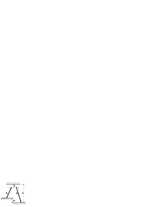
Figure 1: The $\Lambda$-scheme for working energy levels of sodium atoms. The parameters of the scheme are: $\omega_{12}/(2\pi)=1772\mathrm{MHz}$, $\omega/(2\pi)=5.1\cdot 10^{14}\mathrm{Hz}$ ($\lambda=589\mathrm{nm}$), and $\Delta$ is the variable detuning from the resonance.

Within the SVEPA, and in the sharp line limit case ($\Delta=0$), the wave equations for two Rabi-frequencies are reduced to the first order PDEs:

$$\partial_{\zeta}\Omega_{a}=i\nu_{0}\,\psi_{3}\psi_{1}^{*},\;\partial_{\zeta}\Omega_{b}=i\nu_{0}\,\psi_{3}\psi_{2}^{*}.\quad$$ (3)

Here $\zeta=z/c,\tau=t-z/c$, and $\nu_{0}$ is a coupling constant, which depends on the density of atoms.

The Schrödinger equation for the amplitudes $\psi_{1,2,3}$ of atomic wave function reads

$$\partial_{\tau}\psi_{1} = \frac{i}{2}\Omega_{a}^{*}\,\psi_{3};$$

$$\partial_{\tau}\psi_{2} = \frac{i}{2}\Omega_{b}^{*}\,\psi_{3};$$ (4)

$$\partial_{\tau}\psi_{3} = -i\gamma\,\psi_{3}+\frac{i}{2}(\Omega_{a}\psi_{1}+\Omega_{b}\psi_{2}).$$

Here $\gamma$ describes the relaxation rate, and we set $\hbar=1$. We can now exclude the amplitudes of the lower levels $\psi_{1,2}$ and rewrite Eqs.(3), (Slow-light solitons revisited) in the form:

$$\frac{1}{\psi_{3}^{*}}\partial_{\tau}\frac{1}{\psi_{3}}\partial_{\zeta}\Omega_{a}=\frac{\nu_{0}}{2}\Omega_{a};$$

$$\frac{1}{\psi_{3}^{*}}\partial_{\tau}\frac{1}{\psi_{3}}\partial_{\zeta}\Omega_{b}=\frac{\nu_{0}}{2}\Omega_{b};$$ (5)

$$\partial_{\tau}|\psi_{3}|^{2}=-\gamma\,|\psi_{3}|^{2}-\frac{1}{2\nu_{0}}\partial_{\zeta}(|\Omega_{a}|^{2}+|\Omega_{b}|^{2}).$$

$$\partial_{\tau}\varphi_{3}=-\frac{1}{2\nu_{0}\,|\psi_{3}|^{2}}(|\Omega_{a}|^{2}\,\partial_{\zeta}\varphi_{a}+|\Omega_{b}|^{2}\,\partial_{\zeta}\varphi_{b}).$$

Here, $\varphi_{a,b,3}$ are the phases of the fields $\Omega_{a,b}$ and $\psi_{3}$, respectively. For simplicity, and without a loss of generality, we assume in Eqs.(Slow-light solitons revisited) that the fields $\Omega_{a,b}$ are real, i.e $\varphi_{a,b}=0$. Therefore, we can choose $\varphi_{3}=0$. Notice that the first two equations are wave equations for the fields in curvilinear space described by the metric depending on the amplitude of the excited state $\psi_{3}$.

To make parameters dimensionless, we measure the time in units of the optical pulse length $t_{p}=1\mu s$ typical for the experiments on the slow-light phenomena Hau et al. (1999). Therefore, the Rabi frequencies are normalized to $\mathrm{MH}z$. The spatial coordinate will be normalized to the spatial length of the pulse slowed down in the medium to several meters per second. According to the linear theory, the group velocity of slow-light pulse is $v_{g}\approx c\frac{\Omega_{0}^{2}}{2\nu_{0}}$. Here $\Omega_{0}$ is a magnitude of the controlling field required in EIT experiments. Typically, this field has a magnitude of order of few megahertz. So, we choose $\Omega_{0}=3$ and $v_{g}=10^{-7}c$ as representative values reported in experiments with BEC of sodium atoms. Hence the pulse spatial length is $l_{p}=v_{g}t_{p}=30\mu m$, and $\zeta$ is normalized to $10^{-13}s$. In the dimensionless units, the coupling constant $\nu_{0}=\frac{\Omega_{0}^{2}}{2}=4.5$.

In the absence of relaxation, i.e. for $\gamma=0$, the system of equations Eqs.(3),(Slow-light solitons revisited) is exactly solvable in the framework of the inverse scattering method (IS) Faddeev and Takhtadjan (1987); Park and Shin (1998); Byrne et al. (2003); Rybin and Vadeiko (2004). In the present work we provide an elementary method to derive slow-light solitons for the case of an arbitrary controlling field.

In the context of slow light phenomena, the system is assumed to be initially in the following stationary state:

$$\Omega_{a}=0,\;\Omega_{b}=\Omega(\tau),\;|\psi_{at}\rangle=|1\rangle.$$ (6)

Notice that the state $|1\rangle$ is a dark-state for the controlling field $\Omega(\tau)$. This means that the atoms do not interact with the field $\Omega(\tau)$ created by the auxiliary laser. The configuration Eq.(6) above corresponds to a typical experimental setup (see e.g. Hau et al. (1999); Liu et al. (2001); Bajcsy et al. (2003)).

We intend to study the dynamics of coupled atom-field modulations in the $\Lambda$-type model, which can preserve their spatial shape to a large extent while propagating in the media. We consider such solutions as a generalization of the dark-state polariton Fleischhauer and Lukin (2000). In the linear theory the probe field only appears in $\Omega_{a}$, whereas in the nonlinear theory it also forms an inseparable nonlinear superposition with the controlling field in the channel $b$. However, in both cases the Rabi-frequency $\Omega_{a}$ describes probe field modulations. Indeed, the field in the channel $a$ induces atomic transitions from the state $|1\rangle$ to the excited state $|3\rangle$. On the other hand, the amplitude of the excited state drives the field $\Omega_{a}$. From the results of linear and nonlinear theories of electromagnetically induced transparency (EIT) Harris (1997); Grobe et al. (1994); Dey and Agarwal (2003); Dutton and Hau (2004); Rybin and Vadeiko (2004); Rybin et al. (2005) we can infer a physically plausible assumption that the population of the upper level is proportional to the intensity of the field in the probe channel $a$, i.e. $|\Omega_{a}|^{2}\sim|\psi_{3}|^{2}$. In the present work we assume that this observation is relevant for slow light phenomena. Therefore, we postulate that

$$|\psi_{3}|^{2}=\frac{2}{\nu_{0}}k|\Omega_{a}|^{2},$$ (7)

where $k$ is an arbitrary parameter.

We emphasize that the imposed constraint Eq.(7) reduces Eqs. (Slow-light solitons revisited) to a simplified nonlinear system, which provides adequate descriptions of the slow light propagation. In this sense the relation Eq.(7) is central for the present work. As we show below this condition is sufficient and necessary for the slow-light solitons to exist. Introducing new notations: $|\Omega_{a}|\equiv e^{-\rho},\Omega_{b}=\eta$, we find from Eq.(Slow-light solitons revisited) together with Eq.(7) that the field $\rho$ satisfies the Liouville equation

$$\partial_{\zeta\tau}\rho=-k\,e^{-2\rho}.$$ (8)

together with the constraint

$$\partial_{\zeta\tau}\eta+\partial_{\tau}\rho\;\partial_{\zeta}\eta=k\,e^{-2\rho}\,\eta,$$ (9)

and an auxiliary equation

$$\left(4k(\partial_{\tau}+\gamma)+\partial_{\zeta}\right)e^{-2\rho}+\partial_{\zeta}\eta^{2}=0.$$ (10)

It is interesting that the Liouville equation Eq.(8) appears in 2D gravity Giacomini and Pinamonti (2003) and describes a gravitational field defined by the metric $g_{ab}=e^{-2\rho}\gamma_{ab}$, where $\gamma_{ab}$ is the 2-dimensional Minkowski metric. This connection to 2D gravity is further emphasized by the observation that any solution of dilatonic equations Giacomini and Pinamonti (2003) satisfies the system of slow-light Eqs.(8), (9). The dilatonic equations have the following form

$$\partial_{\zeta\tau}\rho-\frac{\partial_{\eta}V(\eta)}{4}\,e^{-2\rho}=0,\;\partial_{\zeta\tau}\eta+\frac{V(\eta)}{2}\,e^{-2\rho}=0,$$ (11)

together with the constraint

$$\partial_{\zeta\tau}\eta+2\,\partial_{\tau}\rho\;\partial_{\zeta}\eta=2k{\cal A}\,e^{-2\rho}\;.$$ (12)

Here ${\cal A}(\zeta,\tau)$ is an arbitrary source term and $V(\eta)=4k\left({{\cal A}-\eta}\right)$ plays the role of the dilatonic potential. For the realization ${\cal A}(\zeta,\tau)=\partial_{\tau}m(\tau)$ with an arbitrary function $m(\tau)$, the equations Eqs.(11),(12), and Eq.(10) for $\gamma=0$ can be readily solved, viz.

$$\rho=-\frac{1}{2}\log\left[{\frac{\partial_{\zeta}\,A_{+}(\zeta)\partial_{\tau}\,A_{-}(\tau)}{(1-kA_{+}A_{-})^{2}}}\right],$$ (13)

$$A_{+}(\zeta)=-\frac{1}{k}\exp[-8\varepsilon_{0}k\zeta],$$ (14)

$$A_{-}(\tau)=\exp\left[{2\varepsilon_{0}\int\frac{d\tau}{m^{2}(\tau)+1}}\right],$$ (15)

$$\eta=2(\partial_{\tau}m-m\partial_{\tau}\rho).$$ (16)

The original fields $\Omega_{a,b}$ then read:

$$\Omega_{a}=\frac{2\varepsilon_{0}}{\sqrt{m^{2}(\tau)+1}}\mathrm{sech}(\varphi),$$ (17)

$$\Omega_{b}=\frac{2\varepsilon_{0}\,m(\tau)}{m^{2}(\tau)+1}\tanh(\varphi)+\frac{1}{2}\frac{\partial_{\tau}m(\tau)}{m^{2}(\tau)+1},$$ (18)

$$\varphi=-4k\,\varepsilon_{0}\,\zeta+\int\frac{\,\varepsilon_{0}\,d\tau}{m^{2}(\tau)+1},$$ (19)

where $\varepsilon_{0}$ is a real arbitrary constant defining the amplitude of slow-light soliton. The background field $\Omega(\tau)$ reads:

$$\Omega(\tau)=\frac{\frac{1}{2}\partial_{\tau}m(\tau)-2\varepsilon_{0}\,m(\tau)}{m^{2}(\tau)+1}.$$ (20)

The function $\Omega(\tau)$ describes the controlling field, which governs the dynamics of the system. The time dependence of this function is determined by modulation of the intensity of the auxiliary laser. As can be readily seen, the velocity of the slow-light soliton reads

$$v_{g}=\frac{1}{4k}\frac{1}{m^{2}(\tau)+1}.$$ (21)

For a constant controlling field $\Omega(\tau)=\Omega_{0}$, and in the simplifying approximation $\frac{\Omega_{0}^{2}}{\varepsilon_{0}^{2}}<\!\!<1$, the group velocity of the slow-light soliton conform to the result of linear theory:

$$v_{g}\approx c\frac{\Omega_{0}^{2}}{2\nu_{0}}.$$ (22)

Expression Eq. (22) immediately suggests that the signal stops, when $\Omega_{0}=0$. Therefore, this expression is the main motivational source for the works on slow-light solitons (see Rybin and Vadeiko (2004),Rybin et al. (2005) and references therein). We envisage the following dynamics scenario. We assume that the slow-light soliton was created in the system before the time $\tau=0$ and is propagating on the background of the constant controlling field $\Omega_{0}$. Suppose that at the moment $\tau=0$ the laser source of the controlling field is switched off. We assume that after this moment the background field will decay reasonably rapidly, as described by a ”switch-off” function $f(\tau)$. The front of the vanishing controlling field, described by the function $f(\tau)$, will then propagate into the medium, starting from the point $\zeta=0$, where the laser is placed. The state of the quantum system Eq.(6) is dark for the controlling field. Therefore the medium is transparent for the spreading front of the vanishing field, which then propagates with the speed of light, eventually overtaking the slow-light soliton and stopping it. To realize this scenario, we assume the controlling field $\Omega(\tau)$ to be constant $\Omega_{0}$ for negative $\tau$ and a $\tau$ dependent switch-off function $f(\tau)$ for positive $\tau$, i.e. $\Omega(\tau)=\Omega_{0}\Theta(-\tau)+f(\tau)\Theta(\tau)$. Here $\Theta(\tau)$ is the Heaviside step function, while $f(0)=\Omega_{0}$. In this setting, the distance that the soliton travels until full stop is

$${\cal L}=\frac{1}{4k}\int_{0}^{\infty}\!\!\!\frac{d\tau}{m^{2}(\tau)+1}.$$ (23)

This distance designates a geometrical point in the medium, where the slow-light soliton disappears, writing itself into the medium as a standing memory bit in the form of a localized polarization cluster.

From Eq.(20) a number of exactly solvable regimes for the stopping of the slow-light soliton can be identified. For $m(\tau)=e^{\alpha\,\tau}$ and $\tau>0,\;\alpha>0$, we obtain $f(\tau)=\left(\frac{\alpha}{4}-\varepsilon_{0}\right)\,\mathrm{sech}(\alpha\,\tau)$ and

$${\cal L}=\frac{1}{8\alpha k}\ln 2\;.$$

Hence, the slower the field decays to zero, i.e. for smaller $\alpha$, the longer the distance that the soliton travels in the medium is. Another physically interesting case $f(\tau)=\Omega_{0}e^{-\alpha\tau}$ was discussed in Rybin et al. (2005).

Discussion. In this paper we derived the slow-light soliton from the sufficient condition Eq.(7). In fact, the inverse scattering analysis as applied in Rybin et al. (2005) to Eqs.(3),(Slow-light solitons revisited) shows that for slow-light solitons a stronger condition holds, namely

$$\psi_{3}=-\frac{1}{2|\lambda-\Delta|}\Omega_{a},$$ (24)

where $\lambda$ is a complex number parameterizing the soliton (in our case $\lambda=i\varepsilon_{0}$). This means that the condition Eq.(7) is also the necessary condition for the slow-light solitons to exist with $k=\frac{\nu_{0}}{8|\lambda-\Delta|^{2}}$.

In a forthcoming publication we will explain a fascinating analogy between the stopping of a slow-light soliton and the formation of a black hole in 2D gravity.

References

- Hau et al. (1999) L. N. Hau, S. E. Harris, Z. Dutton, and C. H. Behroozi, Lett. to Nature 397, 594 (1999).
- Liu et al. (2001) C. Liu, Z. Dutton, C. H. Behroozi, and L. V. Hau, Lett. to Nature 409, 490 (2001).
- Phillips et al. (2001) D. F. Phillips, A. Fleischhauer, A. Mair, R. L. Walsworth, and M. D. Lukin, Phys. Rev. Lett. 86, 783 (2001).
- Bajcsy et al. (2003) M. Bajcsy, A. S. Zibrov, and M. D. Lukin, Lett. to Nature 426, 638 (2003).
- Braje et al. (2003) D. A. Braje, V. Balic, G. Y. Yin, and S. E. Harris, Phys. Rev. A 68, 041801(R) (2003).
- Mikhailov et al. (2004) E. E. Mikhailov, V. A. Sautenkov, Y. V. Rostovtsev, and G. R. Welch, J. Opt. Soc. Am. B 21, 425 (2004).
- Turukhin et al. (2002) A. V. Turukhin, V. S. Sudarshanam, M. S. Shahriar, J. A. Musser, B. S.Ham, and P. R. Hemmer, Phys. Rev. Lett. 88, 023602 (2002).
- Bigelow et al. (2003) M. S. Bigelow, N. N. Lepeshkin, and R. W. Boyd, Science 301, 200 (2003).
- Soljacic and Joannopoulos (2004) M. Soljacic and J. D. Joannopoulos, Nature Materials 3, 213 (2004).
- Kocharovskaya et al. (2001) O. Kocharovskaya, Y. Rostovtsev, and M. O. Scully, Phys. Rev. Lett. 86, 628 (2001).
- Dutton and Hau (2004) Z. Dutton and L. V. Hau, Phys. Rev. A 70, 053831 (2004).
- Harris (1997) S. E. Harris, Phys. Today 50(7), 36 (1997).
- Lukin (2003) M. D. Lukin, Rev. Mod. Phys. 75, 457 (2003).
- Grobe et al. (1994) R. Grobe, F. T. Hioe, and J. H. Eberly, Phys. Rev. Lett. 73, 3183 (1994).
- Eberly (1995) J. H. Eberly, Quant. Semiclass. Opt. 7, 373 (1995).
- Andreev (1998) A. V. Andreev, JETP 86, 412 (1998).
- Dey and Agarwal (2003) T. N. Dey and G. S. Agarwal, Phys. Rev. A 67, 033813 (2003).
- Kozlov and Eberly (2000) V. V. Kozlov and J. H. Eberly, Opt. Commun. 179, 85 (2000).
- Dutton et al. (2001) Z. Dutton, M. Budde, C. Slowe, and L. V. Hau, Science 293, 663 (2001).
- Matsko et al. (2001) A. B. Matsko, Y. V. Rostovtsev, O. Kocharovskaya, A. S. Zibrov, and M. O. Scully, Phys. Rev. A 64, 043809 (2001).
- Faddeev and Takhtadjan (1987) L. D. Faddeev and L. A. Takhtadjan, Hamiltonian Methods in the Theory of Solitons (Springer, Berlin, 1987).
- Park and Shin (1998) Q. H. Park and H. J. Shin, Phys. Rev. A 57, 4643 (1998).
- Byrne et al. (2003) J. A. Byrne, I. R. Gabitov, and G. Kovačič, Physica D 186, 69 (2003).
- Rybin and Vadeiko (2004) A. V. Rybin and I. P. Vadeiko, Journal of Optics B: Quantum and Semiclassical Optics 6, 416 (2004).
- Fleischhauer and Lukin (2000) M. Fleischhauer and M. D. Lukin, Phys. Rev. Lett. 84, 5094 (2000).
- Rybin et al. (2005) A. V. Rybin, I. P. Vadeiko, and A. R. Bishop, Phys. Rev. E 72, 026613 (2005).
- Giacomini and Pinamonti (2003) A. Giacomini and N. Pinamonti, J. High Energy Phys. 02, 014 (2003).