Optical parametric oscillation under injection of orbital angular momentum

Abstract

We present a theoretical model for the spatial mode dynamics of an optical parametric oscillator under injection of orbital angular momentum. This process is then interpreted in terms of an interesting picture based on a Poincaré representation of first order spatial modes. The spatial properties of the down-converted fields can be easily understood from their symmetries in this geometric representation. By considering the adiabatic mode conversion of the injected signal, we also predict the occurrence of a geometric phase conjugation in the down-converted beams. An experimental setup to measure this effect is proposed.

I Introduction

Orbital angular momentum exchange in parametric amplification and oscillation has attracted a significant attention recently, both for its fundamental aspects as well as for its potential applications to quantum information processing. The first attempt to observe the transfer of orbital angular momentum (OAM) from the pump beam to the down converted beams was made by Arlt et al. in the spontaneous process, where the far field did not show the typical profile of an optical vortex.arlt Later, this problem was elucidated by Mair et al who investigated the same process in the photocount regime.Mair They were able to demonstrate that the coincidence counts between twin photons generated by spontaneous parametric down conversion was subjected to OAM conservation. A further insight is given in ref. Caetano, , where it was shown that parametric amplification in the stimulated process is also subjected to OAM conservation. There, an interpretation in terms of transverse phase conjugation was provided.nossoprl In ref. Martinelli, , the macroscopic transfer of OAM from the pump beam to one of the down converted beams was demonstrated in the operation of an optical parametric oscillator (OPO) above threshold. In that case, cavity mode selection was shown to play a crucial role in the OAM exchange.

An important feature of optical beams bearing OAM is the geometric phase, or Berry’s phase,berry associated with cyclic transformations implemented with astigmatic mode converters,HELO ; russos first predicted by van Enk,Enk and then experimentaly demonstrated by Galvez et al.Galvez This geometric phase is related to closed paths in a Poincaré sphere representation of optical beams,poincaresphere and is the orbital equivalent of Pancharatnam’s phase which is associated with cyclic transformations on the polarization state of light.pancharatnam There has been a renewed interest on geometric phases lately due to recent proposals of geometric quantum computation.quantcomp1 ; quantcomp2 The role of Pancharatnam’s phase in nonclassical two-photon interference and the interplay between geometric and dynamical phase was discussed by J. Brendel et al.brendel They showed that the geometric phase acquired by the photon pair depends on the initial polarization state of the two photons.

The generation of discrete multidimensional entanglement by parametric down conversion with optical beams bearing OAM has been discussed in the literature.vaziri ; steve ; Barbosa In contrast to cavity free parametric down conversion, OPOs are an efficient source of continuous variable entanglement in the quadratures of intense optical beams.silvania ; bowen Therefore, parametric down conversion is a reliable source of quantum entanglement, while geometric phases are a potential tool for quantum computation. However, the properties of the geometric phase associated with OAM in parametric down-conversion has not been investigated yet. In this article we start to combine these ideas by studying the classical properties of down converted beams generated by an injected OPO when adiabatic mode conversions are performed in the seed beam. An effect of geometric phase conjugation is predicted which is directly related to a symmetry between the down converted beams in the Poincaré representation.poincaresphere We also propose an experimental setup for measuring this effect from the mutual interference between the down-converted beams. This geometric phase conjugation is equivalent to the time reversal of the Pancharatnam’s phase as observed in four wave mixing by Tompkin et al.chiao Our work provides a first approach to the problem of geometric phase conjugation in parametric oscillation and opens the possibility for a future investigation in the quantum domain.

II Poincaré representation

It is well known that polarization states of a monochromatic light beam can be completely caracterized by the Stokes parameters and mapped on the Poincaré sphere. As van Enk suggests in his paper,Enk there is a correspondence between the polarization states and the first order transverse modes of the electromagnetic field. Based on this correspondence Padgett and Courtial propose a set of Stokes parameters and an equivalent Poincaré representation for the first order transverse modes.poincaresphere

$$p_{1} = \dfrac{I_{HG_{0^{\circ}}}-I_{HG_{90^{\circ}}}}{I_{HG_{0^{\circ}}}+I_{HG_{90^{\circ}}}}$$ (1)

$$p_{2} = \dfrac{I_{HG_{45^{\circ}}}-I_{HG_{135^{\circ}}}}{I_{HG_{45^{\circ}}}+I_{HG_{135^{\circ}}}}$$ (2)

$$p_{3} = \dfrac{I_{LG_{+}}-I_{LG_{-}}}{I_{LG_{+}}+I_{LG_{-}}}\quad,$$ (3)

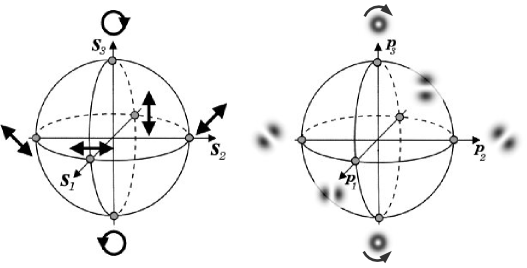
Figure 1: Poincaré sphere for polarization states (left) and first order transverse modes (right). Notice the correspondence between circular polarization states and LG modes, placed on the poles, and linear polarization states and HG modes, placed on the equator.

are the Stokes parameters describing a spatial profile belonging to the subspace of first order transverse modes. In a mode decomposition of the beam profile, $I_{\beta}$ is the square modulus of the coefficient of mode $\beta$. The first order modes are labeled so that $LG_{\pm}$ represents the first order Laguerre-Gaussian (LG) mode with topological charge $\pm 1$, respectively. $HG_{\theta}$ represents a first order Hermite-Gaussian (HG) mode rotated by an angle $\theta$ around the propagation axis. In fig. (1) we can see the Poincaré sphere for polarization states of a monochromatic beam and the equivalent representation for the first order transverse modes. The cartesian coordinates on the sphere are the respective Stokes parameters.

III Transverse mode dynamics

III.1 Equations of motion

We now derive the dynamical equations for an optical parametric oscillator (OPO) operating under cavity conditions such that the pump laser is matched to a $TEM_{00}$ cavity mode and the down-converted beams are amplified with spatial profiles belonging to the first order modes subspace. This situation can be realized by a suitable tunning of the OPO cavity, combined with temperature control of the nonlinear crystal. Therefore, the intracavity pump field $E_{p}(\vec{r})$ can be written as

$$E_{p}(\vec{r})=\alpha_{p}\psi_{00}(\vec{\rho},z)\;,$$ (4)

where $\alpha_{p}$ is the pump amplitude and $\psi_{00}(\vec{\rho},z)$ is the $TEM_{00}$ mode profile.

Now, let us decompose the intracavity signal and idler fields $E_{j}(\vec{r})$ ($j=s,i$) into a linear superposition of first order LG modes:

$$E_{j}(\vec{r})=\alpha^{j}_{+}\psi_{+}(\vec{\rho},z)+\alpha^{j}_{-}\psi_{-}(\vec{\rho},z)\quad,$$ (5)

where $\psi_{\pm}(\vec{\rho},z)$ represent the spatial profiles of the first order LG modes with topological charges $\pm 1$ respectively, and $\alpha^{j}_{\pm}$ are the corresponding intracavity mode amplitudes.

We will consider the dynamics of an injected OPO where two input fields are sent to the OPO cavity. The pump input is mode matched to the $TEM_{00}$ mode and is described by the complex amplitude $\alpha^{p}_{in}\,$. We also assume an incoming seed at the signal field which is prepared in a spatial mode corresponding to a given point in the Poincaré sphere. The input seed is then decribed by two complex amplitudes $\alpha_{+}^{s(in)}$ and $\alpha_{-}^{s(in)}$ which are its components in the Laguerre-Gaussian basis.

In terms of the mode amplitudes, the dynamical equations for the injected OPO are fabre

$$\dfrac{\text{{d}}\alpha_{p}}{\text{{d}}t}=-(\kappa_{p}+i\Delta_{p})\alpha_{p}+\chi\left(\alpha_{+}^{s}\alpha_{-}^{i}+\alpha_{-}^{s}\alpha_{+}^{i}\right)+\eta_{p}\alpha^{p}_{in}$$

$$\dfrac{\text{{d}}\alpha^{s}_{+}}{\text{{d}}t}=-(\kappa+i\Delta)\alpha_{+}^{s}-\chi\alpha_{-}^{i*}\alpha_{p}+\eta_{s}\alpha^{s(in)}_{+}$$

$$\dfrac{\text{{d}}\alpha^{s}_{-}}{\text{{d}}t}=-(\kappa+i\Delta)\alpha_{-}^{s}-\chi\alpha_{+}^{i*}\alpha_{p}+\eta_{s}\alpha^{s(in)}_{-}$$ (6)

$$\dfrac{\text{{d}}\alpha^{i}_{+}}{\text{{d}}t}=-(\kappa+i\Delta)\alpha_{+}^{i}-\chi\alpha_{-}^{s*}\alpha_{p}$$

$$\dfrac{\text{{d}}\alpha^{i}_{-}}{\text{{d}}t}=-(\kappa+i\Delta)\alpha_{-}^{i}-\chi\alpha_{+}^{s*}\alpha_{p}\quad,$$

where $\kappa_{p}$ and $\Delta_{p}$ are, respectively, the cavity damping rate and the frequency detuning for the pump field; $\kappa$ and $\Delta$ are, respectively, the common cavity damping rate and frequency detunning for the down-converted fields; and the constants $\eta_{j}=\sqrt{T_{j}}/\tau_{j}$ $(j=p,s)$ are the coupling between the input fields and the fields inside the cavity. $T_{j}$ and $\tau_{j}$ are, respectively, the input mirror transmition coefficient and the cavity round trip time for each field. The nonlinear coupling constant $\chi$ rules the energy exchange between pump and down-converted fields. It is proportional to the spatial overlap between the transverse modes and to the effective second-order nonlinear susceptibility of the cristal.fabre

III.2 Free running OPO

It is interesting to consider first the case of a free running OPO, for which we take $\alpha_{\pm}^{s(in)}=0\,$. For simplicity, we shall assume resonant operation ($\Delta=\Delta_{p}=0$). In this case, the steady state solution of the dynamical equations gives

$$|\alpha^{s}_{+}|=|\alpha^{i}_{-}|=A\quad,$$

$$|\alpha^{s}_{-}|=|\alpha^{i}_{+}|=B\quad,$$ (7)

where $A$ and $B$ are unknown constants. Their individual values are not fixed by the dynamical equations and somehow depend on the initial conditions. However, the total signal and idler intensities are well defined, as we shall see shortly. This degeneracy is reminiscent of the implicit symmetry assumed in the dynamical equations. If cavity and/or crystal anisotropies are considered, then a rather more complicated scenario shows up as discussed in ref.Martinelli, .

Another degeneracy becomes evident when we consider the steady state values for the phases of the modes amplitudes. By taking $\theta^{p}_{in}=0\,$, we arrive at

$$\theta^{p}=0\quad,$$

$$\theta^{s}_{+}+\theta^{i}_{-}=0\quad,$$ (8)

$$\theta^{s}_{-}+\theta^{i}_{+}=0\quad.$$

Again, the individual values of $\theta^{s}_{\pm}$ and $\theta^{i}_{\pm}$ are not fixed by the dynamical equations and should also depend on the initial conditions.

It is instructive to look at these degeneracies in terms of the Poincaré representation of transverse modes. Solving the steady state equations for the intracavity pump intensity $I_{p}\equiv|\alpha_{p}|^{2}$ we obtain the usual clipping value

$$I_{p}=\left(\frac{\kappa}{\chi}\right)^{2}\quad.$$ (10)

The stationary value of the total intensity of each down converted field is

$$I_{s}=I_{i}=A^{2}+B^{2}=\frac{\chi}{\kappa_{p}}\left(\frac{\eta_{p}}{\kappa_{p}}|\alpha^{p}_{in}|-\frac{\kappa}{\chi}\right)\quad,$$ (11)

where $I_{j}\equiv|\alpha^{j}_{+}|^{2}+|\alpha^{j}_{-}|^{2}$ for $j=s,i\,$. Now, one can easily obtain the stationary values of the Stokes parameters for signal and idler:

$$p^{s}_{1}=p^{i}_{1} = \frac{-2AB}{A^{2}+B^{2}}\cos\Delta\theta\quad,$$

$$p^{s}_{2}=p^{i}_{2} = \frac{-2AB}{A^{2}+B^{2}}\sin\Delta\theta\quad,$$ (12)

$$p^{s}_{3}=-p^{i}_{3} = \frac{A^{2}-B^{2}}{A^{2}+B^{2}}\quad,$$

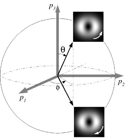
Figure 2: Correlation imposed by optimal spatial overlap and orbital angular momentum conservation. Signal and idler are represented by two points on the Poincaré sphere symmetrically disposed with respect to the equatorial plane.

where $\Delta\theta\equiv\theta^{s}_{+}-\theta^{s}_{-}=\theta^{i}_{+}-\theta^{i}_{-}$. Therefore, the Stokes parameters of signal and idler fields correspond to points on the Poincaré sphere symmetrically disposed with respect to the equatorial plane, as described in fig.2. Since $A$, $B$ and $\Delta\theta$ are not fixed, they are free to diffuse and the steady state for the down converted fields can fall at any pair of points on the sphere, as far as they respect this symmetry. Physically, it means that signal and idler have the same intensity distribution, and therefore optimal spatial overlap, but opposite helicities due to OAM conservation.

Of course, conservation laws are connected to symmetries. In the dynamical equations (6) we have implicitly assumed that the OPO cavity and crystal present cylindrical symmetry. The main anisotropy present in an OPO is the crystal birrefringence. In ref.Martinelli, , the operation of a type-II OPO driven by a Laguerre-Gaussian pump was observed for the first time with transfer of OAM to the idler beam, but not to the signal. For a type-II OPO, signal and idler have orthogonal polarizations, and astigmatic effects induced by the crystal birrefingence prevents the OAM transfer to the signal beam. In fact, as discussed in ref.Martinelli, , a birrefringence dependent astigmatism will cause a frequency split between transverse modes that conserve OAM. For this reason, we will propose an experimental setup based on a type-I OPO, where signal and idler have the same polarization.

The treatment of the nondeterministic dynamics with the addition of noise terms to the dynamical equations will be left for a future investigation. However, we can built a physical picture from the Poincaré representation which allows us to infere some of the main characteristics of the noisy evolution. In fact, the addition of noise should drive the down converted fields along random trajectories in the Poincaré sphere. This is analogous to the random trajectory delineated by the electric field phasor in a geometric representation of laser phase diffusion in the complex plane. In analogy, we can think of random trajectories in the Poincaré sphere as a mode diffusion. Of course, higher order modes may play an important role in the noisy evolution of the free running OPO, and a considerable improvement of the model might be necessary. However, in the case of an injected OPO, higher order modes may still contribute to noise but not to the macroscopic behavior of the amplified modes.

III.3 Injected OPO

Let us now consider a signal seed prepared in an arbitrary superposition of first order modes represented on the Poincaré sphere by the polar and azimuth angles $\theta$ and $\phi$, as shown in fig. 2. The injected signal is then represented by the following amplitudes:

$$\alpha_{+}^{s(in)} = \sqrt{I_{s}^{in}}\cos\left(\frac{\theta}{2}\right)e^{-i\frac{\phi}{2}}\quad,$$ (13)

$$\alpha_{-}^{s(in)} = \sqrt{I_{s}^{in}}\sin\left(\frac{\theta}{2}\right)e^{i\frac{\phi}{2}}\quad.$$ (14)

With this choice for the injection field, the dynamical equations are simplified by the definition of a new set of transformed amplitudes $\alpha_{j}$ and $\alpha^{\prime}_{j}$ $(j=s,i)$ given by:

$$\alpha_{s} = \cos\left(\frac{\theta}{2}\right)e^{i\frac{\phi}{2}}\alpha^{s}_{+}+\sin\left(\frac{\theta}{2}\right)e^{-i\frac{\phi}{2}}\alpha^{s}_{-}$$

$$\alpha_{i} = \sin\left(\frac{\theta}{2}\right)e^{i\frac{\phi}{2}}\alpha^{i}_{+}+\cos\left(\frac{\theta}{2}\right)e^{-i\frac{\phi}{2}}\alpha^{i}_{-}$$

$$\alpha^{\prime}_{s} = -\sin\left(\frac{\theta}{2}\right)e^{i\frac{\phi}{2}}\alpha^{s}_{+}+\cos\left(\frac{\theta}{2}\right)e^{-i\frac{\phi}{2}}\alpha^{s}_{-}$$ (15)

$$\alpha^{\prime}_{i} = \cos\left(\frac{\theta}{2}\right)e^{i\frac{\phi}{2}}\alpha^{i}_{+}-\sin\left(\frac{\theta}{2}\right)e^{-i\frac{\phi}{2}}\alpha^{i}_{-}\quad.$$

The dynamical equations can be rewritten in terms of the transformed amplitudes and one can easily show that the steady state solutions for $\alpha^{\prime}_{j}$ vanish (see appendix). Therefore, only three complex amplitudes $\alpha_{p}$, $\alpha_{s}$ and $\alpha_{i}$ are left.

The new equations of motion are

$$\dfrac{d\alpha_{p}}{dt}=-(\kappa_{p}+i\Delta_{p})\alpha_{p}+\chi\alpha_{s}\alpha_{i}+\eta_{p}\alpha^{in}_{p}$$

$$\dfrac{d\alpha_{s}}{dt}=-(\kappa+i\Delta)\alpha_{s}-\chi\alpha^{*}_{i}\alpha_{p}+\eta_{s}\sqrt{I_{s}^{in}}$$ (16)

$$\dfrac{d\alpha_{i}}{dt}=-(\kappa+i\Delta)\alpha_{i}-\chi\alpha^{*}_{s}\alpha_{p}\quad.$$

The stationary behavior is obtained from the steady-state solutions of eqs. (III.3). We shall consider, for simplicity, that the interacting fields are resonant with the optical cavity ($\Delta=\Delta_{p}=0$). By setting the time derivatives equal to zero in the dynamical equations, we arrive at a set of algebraic equations which can be solved for the steady-state amplitudes.

The steady-state solutions for the down-converted modes can be put in a simple form in terms of the pump mode steady-state solution,

$$\alpha_{s} = \frac{\eta_{s}\rho\sqrt{I_{s}^{in}}}{(\kappa^{2}-\chi^{2}|\alpha_{p}|^{2})}$$ (17)

$$\alpha_{i} = \frac{-\eta_{s}\chi\sqrt{I_{s}^{in}}\alpha_{p}}{(\kappa^{2}-\chi^{2}|\alpha_{p}|^{2})}\quad.$$ (18)

The solutions for the modulus $|\alpha_{p}|$ of the pump mode amplitude are given by the roots of a fifth order polynomial

$$b^{2}|\alpha_{p}|+\left(|\alpha_{p}|-a\right)\left(|\alpha_{p}|-\dfrac{\kappa}{\chi}\right)^{2}\left(|\alpha_{p}|+\dfrac{\kappa}{\chi}\right)^{2}=0\quad,$$

where $a=\eta_{p}|\alpha_{p}^{in}|/\kappa_{p}$, and $b=\eta_{s}\kappa|\alpha_{s}^{in}|/(\chi\sqrt{\kappa\kappa_{p}})$.

There is no algorithm to find analytical expressions for the roots of a fifth order polynomial. However, simple approximate expressions can be given for some operation regimes of the OPO. In ref.Coutinho, these expressions are presented together with a linear stability analysis showing that the stable solutions satisfy $|\alpha_{p}|<\kappa/\chi\,$.

IV Geometric phase conjugation and an experimental proposal

The geometric phase was first discovered in 1956 by S. Pancharatnam.pancharatnam This kind of geometric phase appears when a monochromatic light beam passes through a cyclic transformation on its polarization state, represented by a closed path on the Poincaré sphere. The geometric phase acquired by the beam is equal to minus one half the solid angle enclosed by the path.

In analogy to Pancharatnam phase, van Enk proposed the appearence of a geometric phase as we make cyclic transformations on transverse modes,Enk even though the polarization state and the propagation direction of the beam do not change. Such transformations can be made with the help of astigmatic mode converters HELO and spatial rotators (Dove prisms). In Galvez et al,Galvez the existence of van Enk’s geometric phase was first demonstrated through the interference between a first-order mode following cyclic mode conversions and a $TEM_{00}$ reference beam. As in the case of Pancharatnam’s phase, the geometric phase aquired in the cyclic evolution is equal to minus one half the solid angle enclosed by the path followed in the Poincaré representation of first order spatial modes.

Now, let us consider the injected OPO described above. A cyclic transformation performed adiabatically on the injection mode, equivalent to a slow variation of $\theta$ and $\phi$ in eqs. (13) and (14), will cause the down converted beams to perform closed paths on the Poincaré sphere. The Stokes parameters of the down-converted beams can be readily calculated by inverting eqs. (15) and inserting the steady state solutions in definitions (1)-(3):

$$p^{s}_{1} = p^{i}_{1}=\sin\theta\cos\phi\quad,$$ (19)

$$p^{s}_{2} = p^{i}_{2}=-\sin\theta\sin\phi\quad,$$ (20)

$$p^{s}_{3} = -p^{i}_{3}=\cos\theta\quad.$$ (21)

Since signal and idler have opposite signs of $p_{3}$, they will perform symmetric paths with respect to the equator of the Poincaré sphere. Closed paths will be followed in opposite senses with respect to the unit vector normal to the sphere, as described in fig.3. Therefore, the geometric phase acquired by the idler field will be the conjugate of the one acquired by the signal.

However, there is a subtle difference between this geometric phase and the one described in refs.Enk, ; Galvez, ; poincaresphere, . In that case, the geometric phase is aquired along the propagation of the optical beam through a sequence of mode converters that implement a cyclic operation. Therefore, the time scale involved in the whole process is given by the time of flight of the optical beam through the setup and the notion of adiabatic transport is not clear. In our case, the idea is to drive the OPO adiabatically through a cyclic transformation during a time scale slow enough to consider the system approximately stationary at each moment. More precisely, we propose to inject a type-I OPO with an optical beam initially prepared in a given point of the Poincaré sphere, and to modify the setup adiabatically in order to drive the OPO slowly through a cyclic evolution. The relative geometric phase aquired by the down-converted beams can then be measured by their mutual interference. The choice of type-I phase match is important to avoid the astigmatic effects discussed above.

Consider, for example, the setup sketched in fig.4a. A dual wavelength laser source provides both the OPO pump at the visible wavelength (VIS) and the injection seed at the infrared (IR). The injection beam is sent to a mode preparation setup where arbitrary modes on the Poincaré sphere can be produced. The mode preparation settings are then adiabatically varied in order to drive the OPO injection over a given path on the sphere. The adiabatic character of this evolution is important to ensure that the idler beam produced by the OPO preserves its symmetry with respect to the signal beam. Therefore, the mode preparation settings must be varied in a time scale much longer than the cavity lifetime $2\pi/\kappa$ for the down-converted beams. After the OPO, the IR beams are transmitted through a dichroic mirror (DM), where they are separated from the visible pump beam, and spatially interfere on the screen of a CCD camera. In the case of a type II OPO, the down-converted beams have orthogonal polarizations, so that a polarizer (POL) oriented at $45^{o}$ with respect to their polarizations must be introduced in order to provide interference.

The mode preparation setup is described in fig.4b. Two Laguerre-Gaussian modes with opposite helicities and orthogonal polarizations are sent to a phase shifter which consists of a Sagnac interferometer with a polarizing beam splitter (PBS) as the input/output port, two quarter-wave plates and one half-wave plate. The quarter-wave plates are oriented at $45^{o}$ with respect to the horizontal axis. The orientation of the half-wave plate can be varied and it is convenient to write it as $\phi/4-45^{0}\,$. With this configuration, the relative phase between the counter-propagating beams in the output of the phase shifter is $\phi\,$. Finally, after recombining at the output of the Sagnac interferometer, the two phase shifted modes pass through a second half-wave plate at a variable orientation $\theta/4$ and another polarizing beam splitter. The resulting field profile is

$$E_{s}^{in}=\sqrt{I_{s}^{in}}\left[e^{-i\phi/2}\,\cos\left(\theta/2\right)\,\psi_{+}(\vec{\rho},z)+e^{i\phi/2}\,\sin\left(\theta/2\right)\,\psi_{-}(\vec{\rho},z)\right]\;,$$ (22)

which is equivalent to the injection amplitudes given by eqs.(13) and (14). Therefore, the injection field can be prepared at any point on the Poincaré sphere by proper orientation of the half wave plates.

After the cyclic transformation, the injection seed follows the path $ABCA$ (fig.3) corresponding to a solid angle $\Omega=\Delta\phi$ in the Poincaré sphere, where $\Delta\phi$ is the azimuthal angle enclosed by the path on the equator. The geometric phase aquired by the injected signal is $\gamma_{s}=-\Delta\phi/2\,$. The idler beam is then adiabatically driven over the symmetric path $DBCD\,$, so that a geometric phase $\gamma_{i}=-\gamma_{s}=\Delta\phi/2$ is aquired by the idler. Therefore, the phase difference between the down-converted beams is increased by $\Delta\phi$ and can be measured by the change in their mutual interference pattern, as shown in fig.5. After the cyclic transformation, the memory of the adiabatic evolution is registered as a rotation of the mutual interference pattern.

V Conclusions

In conclusion, we studied the classical dynamics of an optical parametric oscillator injected with a signal seed initially prepared in a transverse mode carrying orbital angular momentum. By the use of a Poincaré sphere representation, we stablished a transverse mode symmetry between the down converted beams. We also predicted an effect of geometric phase conjugation when adiabatic mode conversions, following closed paths in the Poincaré sphere, are performed on the injected beam. An experimental setup for measuring this effect was proposed and one of its interesting aspects is the memory of the adiabatic evolution registered in the image of an interference pattern. The investigation of this effect in the quantum domain is left for a future work.

Appendix

The transformed variables introduced by eqs. 15 allow us to rewrite the dynamical equations with a single injection term:

$$\dfrac{d\alpha_{p}}{dt}=-(\kappa_{p}+i\Delta_{p})\alpha_{p}+\chi^{*}_{ef}\left(\alpha_{s}\alpha_{i}-\alpha^{\prime}_{s}\alpha^{\prime}_{i}\right)+\eta_{p}\alpha^{in}_{p}$$ (23)

$$\dfrac{d\alpha_{s}}{dt}=-(\kappa+i\Delta)\alpha_{s}-\chi_{ef}\alpha^{*}_{i}\alpha_{p}+\eta_{s}\sqrt{I^{in}_{s}}$$ (24)

$$\dfrac{d\alpha_{i}}{dt}=-(\kappa+i\Delta)\alpha_{i}-\chi_{ef}\alpha^{*}_{s}\alpha_{p}$$ (25)

$$\dfrac{d\alpha^{\prime}_{s}}{dt}=-(\kappa+i\Delta)\alpha^{\prime}_{s}-\chi_{ef}\alpha^{\prime*}_{i}\alpha_{p}$$ (26)

$$\dfrac{d\alpha^{\prime}_{i}}{dt}=-(\kappa+i\Delta)\alpha^{\prime}_{i}-\chi_{ef}\alpha^{\prime*}_{s}\alpha_{p}\quad.$$ (27)

This substantially simplifies the steady state solution, which can be readily found from the following algebraic system:

$$\alpha_{p}=\dfrac{\chi}{\kappa_{p}}\left(\alpha_{s}\alpha_{i}-\alpha^{\prime}_{s}\alpha^{\prime}_{i}\right)+\dfrac{\eta_{p}}{\kappa_{p}}\alpha^{in}_{p}$$ (28)

$$\alpha_{s}=-\dfrac{\chi}{\kappa}\alpha^{*}_{i}\alpha_{p}+\dfrac{\eta_{s}}{\kappa}\sqrt{I^{in}_{s}}$$ (29)

$$\alpha_{i}=-\dfrac{\chi}{\kappa}\alpha^{*}_{s}\alpha_{p}$$ (30)

$$\alpha^{\prime}_{s}=-\dfrac{\chi}{\kappa}\alpha^{\prime*}_{i}\alpha_{p}$$ (31)

$$\alpha^{\prime}_{i}=-\dfrac{\chi}{\kappa}\alpha^{\prime*}_{s}\alpha_{p}\quad,$$ (32)

where we assumed $\Delta_{p}=\Delta=0$ for simplicity.

A straightforward algebra with the last two equations, gives

$$\alpha^{\prime}_{s}\left(1-\dfrac{|\chi|^{2}}{\kappa^{2}}|\alpha_{p}|^{2}\right)=0\quad.$$ (33)

One of the solutions is $|\alpha_{p}|^{2}=\kappa^{2}/\chi^{2}$, which is nonphysical since it corresponds to the noninjected case solution for the pump mode. The other one is $\alpha^{\prime}_{s}=0$, which shows that both amplitudes $\alpha^{\prime}_{s}$ and $\alpha^{\prime}_{i}$ vanish. Therefore, the corresponding modes are not amplified and do not oscillate. However, they will certainly contribute to noise but this will be left for a future investigation.

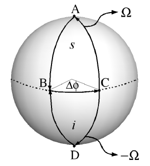
Figure 3: Poincaré representation of the transformations performed on signal and idler beams.

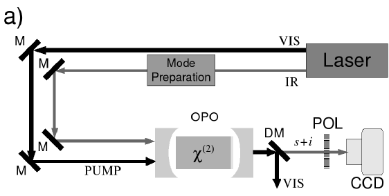
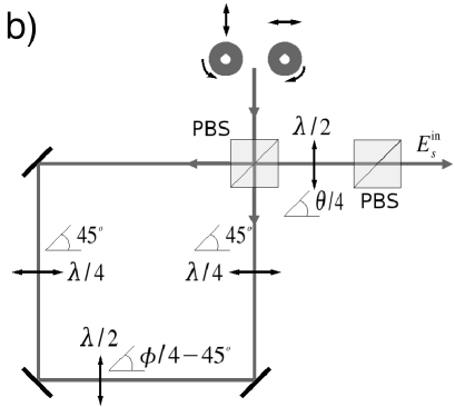
Figure 4: a) A proposed experimental setup for measuring the geometric phase conjugation. M=mirror, DM=dichroic mirror, POL=polarizer. b) Mode preparation setup. PBS=polarizing beam splitter.

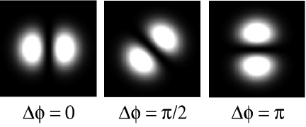
Figure 5: Calculated intereference patterns for different cyclic evolutions of the OPO.

References

- (1) J. Arlt, K. Dholakia, L. Allen, and M. J. Padgett, ”Parametric down conversion for light beams possessing orbital angular momentum,” Phys. Rev. A 59, 3950-3952 (1999).
- (2) A. Mair, A. Vaziri, G. Weihs, and A. Zeilinger, ”Entanglement of the orbital angular momentum states of photons,” Nature (London) 412, 313-316 (2001).
- (3) D.P. Caetano, M.P. Almeida, P.H. Souto Ribeiro, J.A.O. Huguenin, B. Coutinho dos Santos, and A.Z. Khoury, ”Conservation of orbital angular momentum in stimulated down-conversion,” Physical Review A 66, 041801 (Rapid Comm.) (2002).
- (4) P. H. Souto Ribeiro, D. P. Caetano, M. P. Almeida, J. A. Huguenin, B. Coutinho dos Santos, and A. Z. Khoury, ”Observation of image transfer and phase conjugation in stimulated down-conversion,” Phys. Rev. Lett. 87, 133602 (2001).
- (5) M. Martinelli, J. A. O. Huguenin, P. Nussenzveig, and A. Z. Khoury, ”Orbital angular momentum exchange in an optical parametric oscillator,” Phys. Rev. A 70, 013812 (2004).
- (6) M. V. Berry, ”Quantal phase-factors accompanying adiabatic changes,” Proc. R. Soc. London A 392, 45 (1984).
- (7) M. W. Beijersbergen, L. Allen, H. E. L. O. var der Veen, and J. P. Woerdman, ”Astigmatic laser mode converters and transfer of orbital angular momentum,” Opt. Commun. 96, 123-132 (1993).
- (8) E. Abramochkin and V. Volostnikov, ”Beam transformations and nontransformed beams,” Opt. Commun. 83, 123-135 (1991).
- (9) S. J. van Enk, ”Geometric phase, transformations of Gaussian light-beams and angular-momentum transfer,” Opt. Commun 102, 59 (1993).
- (10) E. J. Galvez, P. R. Crawford, H. I. Sztul, M. J. Pysher, P. J. Haglin, and R. E. Williams, ”Geometric phase associated with mode transformations of optical beams bearing orbital angular momentum,” Phys. Rev. Lett. 90, 203901 (2003).
- (11) M. J. Padgett, and J. Courtial, ”Poincare-sphere equivalent for light beams containing orbital angular momentum,” Optics Letters 24, 430, (1999).
- (12) S.Pancharatnam, ”Generalized theory of interference and its applications. Part I. Coherent pencils,” Proc. Ind. Acad. Sci. 44, 247 (1956).
- (13) J. A. Jones, V. Vedral, A. Ekert, and G. Castagnoli, ”Geometric quantum computation using nuclear magnetic resonance,” Nature (London) 403, 869-871 (2000).
- (14) L.-M. Duan, J. I. Cirac, and P. Zoller, ”Geometric manipulation of trapped ions for quantum computation,” Science 292, 1695-1697 (2001).
- (15) J. Brendel, W. Dultz, and W. Martienssen, ”Geometric phases in 2-photon interference experiments,” Phys. Rev. A 52, 2551-2556 (1995).
- (16) A. Vaziri, G. Weihs, and A. Zeilinger, ”Experimental two-photon, three-dimensional entanglement for quantum communication,” Phys. Rev. Lett. 89, 240401 (2002).
- (17) S. P. Walborn, A. N. de Oliveira, R. S. Thebaldi, and C. H. Monken, ”Entanglement and conservation of orbital angular momentum in spontaneous parametric down-conversion,” Phys. Rev. A 69, 023811 (2004).
- (18) H. H. Arnaut and G. A. Barbosa, ”Orbital and intrinsic angular momentum of single photons and entangled pairs of photons generated by parametric down-conversion,” Phys. Rev. Lett. 85, 286 (2000).
- (19) Z. Y. Ou, S. F. Pereira, and H. J. Kimble, ”Realization of the Einstein-Podolsky-Rosen paradox for continuous-variables in nondegenerate parametric amplification,” App. Phys. B 55, 265-278 (1992); Z. Y. Ou, S. F. Pereira, J. Kimble, and K. C. Peng, ”Realization of the Einstein-Podolsky-Rosen paradox for continuous-variables,” Phys. Rev. Lett. 68, 3663-3666 (1992).
- (20) W. P. Bowen, N. Treps, R. Schnabel, and P. K. Lam, ”Experimental demonstration of continuous variable polarization entanglement,” Phys. Rev. Lett. 89, 253601 (2002); W. P. Bowen, R. Schnabel, P. K. Lam, and T. C. Ralph, ”Experimental investigation of criteria for continuous variable entanglement,” Phys. Rev. Lett. 90, 043601 (2003).
- (21) W. R. Tompkin, M. S. Malcuit, R. W. Boyd, and R. Y. Chiao, ”Time reversal of Berry’s phase by optical phase conjugation,” J. Opt. Soc. Am. B 7, 230-233 (1990).
- (22) C. Schwob, P. F. Cohadon, C. Fabre, M. A. M. Marte, H. Ritsch, A. Gatti, and L. Lugiato, ”Transverse effects and mode couplings in OPOS,” Appl. Phys. B 66, 685-699 (1998).
- (23) B. Coutinho dos Santos, K. Dechoum, A. Z. Khoury, L. F. da Silva, and M. K. Olsen, ”Quantum analysis of the nondegenerate optical parametric oscillator with injected signal,” Phys. Rev. A 72, 033820 (2005).