Uniform semiclassical approximations of the nonlinear Schrödinger equation by a Painlevé mapping

Abstract

A useful semiclassical method to calculate eigenfunctions of the Schrödinger equation is the mapping to a well-known ordinary differential equation, as for example Airy’s equation. In this paper we generalize the mapping procedure to the nonlinear Schrödinger equation or Gross-Pitaevskii equation describing the macroscopic wave function of a Bose-Einstein condensate. The nonlinear Schrödinger equation is mapped to the second Painlevé equation ($P_{II}$), which is one of the best-known differential equations with a cubic nonlinearity. A quantization condition is derived from the connection formulae of these functions. Comparison with numerically exact results for a harmonic trap demonstrates the benefit of the mapping method. Finally we discuss the influence of a shallow periodic potential on bright soliton solutions by a mapping to a constant potential.
PACS: 03.65.Ge, 03.65.Sq, 03.75.-b

1 Introduction

In the case of low temperatures, the dynamics of a Bose-Einstein condensate (BEC) can be described in a mean–field approach by the nonlinear Schrödinger equation (NLSE) or Gross–Pitaevskii equation (see, e.g., [1])

$$\left(-\frac{\hbar^{2}}{2M}\frac{\partial^{2}}{\partial x^{2}}+V(x)+g|\psi(x,t)|^{2}\right)\psi(x,t)={\rm i}\hbar\frac{\partial\psi(x)}{\partial t}\,,$$ (1)

where $g$ is the nonlinear interaction strength. Stationary nonlinear eigenstates of the NLSE satisfying $\psi(x,t)=\exp(-{\rm i}\mu t/\hbar)\psi(x)$ fulfill the time-independent NLSE

$$\left(-\frac{\hbar^{2}}{2M}\frac{{\rm d}^{2}}{{\rm d}x^{2}}+V(x)+g|\psi(x)|^{2}\right)\psi(x)=\mu\psi(x)\,.$$ (2)

Analytic solutions of the NLSE are available only for some special cases, among these the free NLSE [2, 3], arrangements of delta-potentials [4, 5, 6] and potentials given by Jacobi elliptic functions [7]. Thus there is a great interest in feasible approximation to the NLSE, among which the most popular one is the Thomas-Fermi approximation for the ground state in a trapping potential.

Recently two semiclassical methods for the calculation of nonlinear eigenstates were proposed. Mention and discuss other semiclassical approaches to the NLSE: Bohr-Sommerfeld quantization [8] and the divergence-free WKB method [9, 10]

In this paper we discuss another semiclassical methods to solve the time-independent NLSE approximately based on a mapping to Painlevé second equation. Special attention will be paid to the shift of the chemical potential $\mu$ of bound states due to the nonlinear mean-field energy. This method provides good results for excited states and it is fairly easy to understand and to use.

We will focus on the one–dimensional case, which arises, for example, in confined geometries (see, e.g., [11] and references therein). Then the effective interaction strength is given by $g=2\hbar^{2}aN/Ma_{\perp}^{2}$, where $a$ is the s-wave scattering length, $a_{\perp}$ is the transverse extension of the condensate and $N$ is the number of atoms [12]. We assume that the wave function is normalized as $\|\psi\|^{2}=1$.

For convenience we rescale the NLSE (2) such that $\hbar=M=1$.This yields the NLSE in the convenient form

$$\frac{{\rm d}^{2}\psi}{{\rm d}x^{2}}=-q^{2}(x)\psi(x)+2g|\psi(x)|^{2}\psi(x)$$ (3)

with $q^{2}(x)=2(\mu-V(x))$.

For the most important case of a harmonic trap $V(x)=m\omega^{2}x^{2}/2$ discussed in section 4 this is achieved by the rescaling the variables as

$$x^{\prime}=x/\ell,\quad\psi^{\prime}=\sqrt{\ell}\psi,\quad g^{\prime}=\ell Mg/\hbar^{2}\quad\mbox{and}\,\mu^{\prime}=\mu/(\hbar\omega)$$ (4)

with the standard length $\ell=\sqrt{\hbar/M\omega}$. The rescaled potential is $V(x)=x^{2}/2$ and the chemical potential is given in units of $\hbar\omega$. To get a feeling for the relevant dimensions consider a BEC of $10^{4}$ atoms with transverse width $a_{\perp}=10\mu m$. This yields a scaled nonlinearity of $g=+20$ for a ${}^{87}{\rm Rb}$ BEC in a trap with axial frequency $\omega=2\pi\times 2{\rm Hz}$ and $g=-20$ for a ${}^{7}{\rm Li}$-BEC in a trap with $\omega=2\pi\times 100{\rm Hz}$.

Finally, let us note that the nonlinear Schrödinger equation also describes the propagation of electromagnetic waves in nonlinear media (see, e.g., [13], ch. 8).

2 The second Painlevé transcendent

One of the most famous ordinary differential equation with a cubic nonlinearity is Painlevé’s second equation or shortly the $P_{II}$ equation (see, e.g. [14, 15]),

$$\frac{{\rm d}^{2}\phi}{{\rm d}y^{2}}=2\sigma\phi^{3}+y\phi\,,\quad\sigma=\pm 1.$$ (5)

The solutions $\phi_{k}(x)$, where the index $k$ refers to the asymptotics at $y\rightarrow+\infty$, are transcendent. In the linear case, which is found for $\sigma=0$, the $P_{II}$ equation reduces to the Airy equation. In fact Airy functions are found in the asymptotic limit (see below).

In textbooks one mostly finds results for the repulsive case $\sigma=+1$. However, asymptotic expansions, which will prove itself as quite useful, are available for both cases [16, 17]. For $y\rightarrow+\infty$ the Painlevé transcendent $\phi_{k}(x)$ vanishes as

$$\phi_{k}(y)\sim k{\rm Ai}(y)$$ (6)

We can restrict ourselves to $k>0$, since equation (5) is invariant under a sign change of $\phi(y)$. Connection formulae, which relate the asymptotic form for $y\rightarrow-\infty$ to the form for $y\rightarrow+\infty$ are well known [16, 17]. For $\sigma=+1$ and $k\geq 1$ the Painlevé transcendent diverges. Otherwise the solution is oscillatory for negative $y$ with asymptotics

$$\phi_{k}(y)\sim d|y|^{-1/4}\sin\left(\dfrac{2}{3}|y|^{3/2}-\dfrac{3}{4}\sigma d^{2}\ln|y|-\theta\right)+\mathcal{O}(|y|^{-7/4}).$$ (7)

The constants depend on the parameter $k$ as

$$d^{2}(k) = -\frac{\sigma}{\pi}\ln(1-\sigma k^{2})$$ (8)

$$\theta(k) = \frac{3}{2}\sigma d^{2}(k)\ln 2+\sigma\arg\left[\Gamma\left(1-\dfrac{1}{2}{\rm i}d^{2}(k)\right)\right]-\dfrac{\pi}{4}.$$ (9)

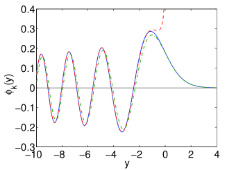
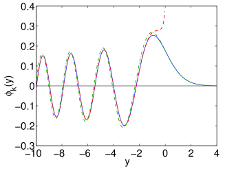
Figure 1: The Painlevé transcendent $\phi_{k}(y)$ (solid blue lines) for $k=0.5$ and $\sigma=+1$ (left) and $\sigma=-1$ (right) in comparison with the asymptotic forms (7) (red dashed line) and $k{\rm Ai}(y)$ (green dash-dotted line).

The form of the second Painleé transcendent is illustrated in figure 1. We plotted the Painlevé transcendent $\phi_{k}(y)$ in comparison with the asymptotic expansions (7) for $y<0$ and (6) for $y>0$ for $k=0.5$ and $\sigma=\pm 1$. One observes that the asymptotic expansions are quite accurate already for small values of $|y|$.

Furthermore, note that the $P_{II}$ equation with $\sigma=+1$ can be written as a Hamiltonian system [15]

$$\frac{{\rm d}\phi}{{\rm d}x}=\frac{\partial{\cal H}}{\partial p}\,,\qquad\frac{{\rm d}p}{{\rm d}x}=-\frac{\partial{\cal H}}{\partial\phi}$$ (10)

with the Hamiltonian function

$${\cal H}=\frac{p^{2}}{2}-\left(\phi^{2}+\frac{x}{2}\right)p-\frac{\phi}{2}.$$ (11)

3 The wedge potential

As a first illustrative example for the application of the $P_{II}$ equation we consider the real-valued nonlinear eigenstates in a wedge potential

$$V(x)=F|x|.$$ (12)

This potential might appear a bit artificial, but it provides a natural and easily understandable example for the nonlinear quantisation using the $P_{II}$ transcendent. Furthermore, the quantum states of cold neutrons in the earth’s gravity potential above a hard wall corresponding to a half-wedge were measured only recently [18].

We consider only real states with a defined parity $\psi(x)=(-1)^{n}\psi(-x)$, such that we can restrict our analysis to the positive real line, $x>0$ and replace $|\psi(x)|^{2}\psi(x)$ by $\psi(x)^{3}$ By the means of a scaling $y=(2F)^{1/3}(x-\mu/F)$ and $\psi=|g|^{-1/2}(2F)^{1/3}\phi$, the NLSE with the wedge potential is transformed to the standard form

$$\frac{{\rm d}^{2}\phi}{{\rm d}y^{2}}=2\sigma\phi^{3}+y\phi$$ (13)

with $\sigma={\rm sign}(g)$. The scaled variable $y$ is negative in the classically allowed region $Fx<\mu$ such that the wavefunction is oscillatory. In the classically forbidden region $Fx>\mu$ one has $y>0$ and the wavefunction vanishes as $\phi(y)\sim k{\rm Ai}(y)$. Note that the differential equation (13) does not depend on the nonlinear parameter $g$ explicitly - this dependence is hidden in the normalization of $\phi_{k}(y)$. Rescaling the normalization condition $\|\psi\|^{2}=1$ yields

$$2\int_{y(x=0)}^{+\infty}|\phi_{k}(y)|^{2}{\rm d}y=\frac{|g|}{(2F)^{1/3}}\,.$$ (14)

The quantisation condition can now be deduced from the asymptotic form (7) of the Painlevé transcendent. Note that the definition of a quantum number is not so straightforward as in the linear case, as new nonlinear eigenstates can emerge and disappear if the nonlinearity $g$ is changed (see, e.g. [19]). However, if we restrict ourselves to the nonlinear eigenstates with a linear counterpart and thus a defined parity, the quantum number can be identified with the number of zeros of the wavefunction. Thus the relevant quantisation condition is that the wavefunction $\psi_{n}(x)$ must have $n$ zeros. Due to the (anti)symmetry $\psi(x)=(-1)^{n}\psi(-x)$, the wavefunction assumes an extremum ($n$ even) or a zero ($n$ odd) at $x=0$.

Using the asymptotic form (7) of the Painlevé transcendent, this condition can now be cast into an explicit form. As the asymptotic form of the $P_{II}$ transcendent is basically given by a sine function, a condition for the argument of this sine function directly follows from the conditions on the wavefunction. In fact, the argument of the sine at $y(x=0)=-2^{1/3}\mu/F^{2/3}$ must equal $(n+1)\pi/2$. Inserting this into equation (7) yields the relevant quantisation condition

$$\frac{(2\mu)^{3/2}}{3F}-\dfrac{3}{4}\sigma d^{2}(k_{n})\ln\left(\frac{2^{1/3}\mu}{F^{2/3}}\right)-\theta(k_{n})=\frac{n+1}{2}\pi,$$ (15)

where $d(k_{n})$ and $\theta(k_{n})$ are given by equations (8) and (9), respectively. The advantage of this method is that the problem of solving a nonlinear boundary value problem is reduced to a single algebraic equation.

However, calculating a nonlinear eigenstate with quantum number $n$ for a given value of the nonlinear parameter $g$ is not so easy. In fact one has to determine the chemical potential $\mu$ so that the quantisation condition (15) and the normalization condition (14) are fulfilled simultaneously. This can be achieved by an iterative method. It is much easier, however, to start from a fixed value of $\mu$. The quantisation condition (15) then yields solutions $k_{n}$ for different quantum numbers $n$. Given these values of $k_{n}$, one can calculate the Painlevé functions $\phi_{k}(y)$ and the effective nonlinear parameter $g_{n}(\mu)$ from the normalization integral (14). Rescaling the variables to $x$ and $\psi$ again directly gives the wavefunction $\psi(x)$.

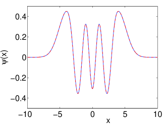
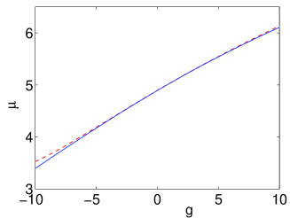
Figure 2: Nonlinear eigenstate with quantum number $n=6$ of the NLSE for a wedge potential $V(x)=|x|$. Left: wavefunction for $g=5$, right: Dependence of the chemical potential on the nonlinearities $g$. The semiclassical results (dashed red line) are compared to numerically exact results (solid blue line).

To test the feasibility of this approach, we consider the nonlinear eigenstate $n=4$ for a wedge potential with $F=1$. The resulting wavefunction is shown in figure 2 on the left-hand side (dashed red line) in comparison with the numerically exact solution (solid blue line). Both wavefunctions are indistinguishable on the scale of drawing. The right side shows the dependence of the chemical potential on the nonlinearity $g$, again in comparison to the numerically exact values. One observes a good agreement. The numerical results for the NLSE solutions were obtained using the standard boundary-value solver bvp4c of MATLAB.

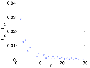
Figure 3: Solution of the NLSE for a wedge potential: Error of the semiclassical calculation of the chemical potential $\mu_{sc}-\mu_{ex}$ in dependence of the quantum number $n$ for $g=5$.

The only error in this calculation results from the replacement of the $P_{II}$ transcendent by its asymptotic form (7). This error vanishes rapidly for larger quantum numbers $n$, which is illustrated in figure 3. The extrema of the $P_{II}$ transcendent are given less accurately by the asymptotic form than the zeros. Thus the error is larger for even quantum number $n$.

4 The harmonic potential

Now we want to extend the quantisation method presented in the previous section to a more important application - the harmonic trap

$$V(x)=\frac{x^{2}}{2}.$$ (16)

A common method used in semiclassics is a comparison of the Schrödinger equation to a well-known differential equation, such as Airy’s equation [20, 21]. Similarly we will map the NLSE for the harmonic trap to the the $P_{II}$ equation.

We use the mapping ansatz

$$\psi(x)=af(x)\phi(y(x)),$$ (17)

well known for the linear Schrödinger equation [21], however with an additional scaling constant $a$. Differentiating twice gives

$$\frac{1}{a}\frac{{\rm d}^{2}\psi}{{\rm d}x^{2}}=\frac{{\rm d}^{2}f}{{\rm d}x^{2}}\phi+2\frac{{\rm d}f}{{\rm d}x}\frac{{\rm d}\phi}{{\rm d}y}\frac{{\rm d}y}{{\rm d}x}+f\frac{{\rm d}\phi}{{\rm d}y}\frac{{\rm d}^{2}y}{{\rm d}x^{2}}+f\left(\frac{{\rm d}y}{{\rm d}x}\right)^{2}\frac{{\rm d}^{2}\phi}{{\rm d}y^{2}}$$ (18)

We demand that the terms proportional to ${\rm d}\phi/{\rm d}y$ cancel, which leads to the condition

$$2\frac{{\rm d}f}{{\rm d}x}\frac{{\rm d}y}{{\rm d}x}+f\frac{{\rm d}^{2}y}{{\rm d}x^{2}}=0\qquad\Rightarrow\;f(x)=\left(\frac{{\rm d}y}{{\rm d}x}\right)^{-1/2}.$$ (19)

Furthermore the term proportional to ${\rm d}^{2}f/{\rm d}x^{2}$ is assumed to be small and can be neglected. Substituting the $P_{II}$ equation (5) and the NLSE (3) into equation (18) finally yields

$$\left(\frac{{\rm d}y}{{\rm d}x}\right)^{2}\left[2\sigma\phi^{3}+y\phi\right]+q^{2}(x)\phi-2ga^{2}\left(\frac{{\rm d}y}{{\rm d}x}\right)^{-1}\phi^{3}=0.$$ (20)

In the linear world, which is given by $g=0$ or $\sigma=0$ respectively, this directly gives a differential equation that determines the mapping $y(x)$. If the nonlinear effects are small, we can neglect the nonlinear terms in the mapping equation which yields

$$\left(\frac{{\rm d}y}{{\rm d}x}\right)^{2}=\frac{-q^{2}(x)}{y(x)}\,.$$ (21)

The scaling constant $a$ is now chosen such that the error due to the neglect of the nonlinear terms in the mapping equation (21) is as small as possible. In the fashion of a least squares fit, $a$ is chosen such that the error

$$\chi^{2}=\int_{-\infty}^{\infty}\left[\sigma\left(\frac{{\rm d}y}{{\rm d}x}\right)^{2}-ga^{2}\left(\frac{{\rm d}y}{{\rm d}x}\right)^{-1}\right]^{2}\phi(y(x))^{6}{\rm d}x$$ (22)

is minimal. This can be done at the end of the calculation, after $\phi(y(x))$ has been determined.

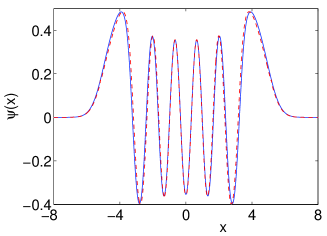
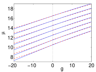
Figure 4: Nonlinear eigenstates of the NLSE in a harmonic potential $V(x)=x^{2}/2$. Left: Wavefunction of the eigenstate with quantum number $n=10$ for $g=10$, right: Dependence of the chemical potential on the nonlinearities $g$ for the eigenstates $n=10-16$. The semiclassical results (dashed red line) are compared to numerically exact results (solid blue line).

This mapping can now be used to approximately calculate eigenstates in symmetric single minimum potentials at $x=0$, e.g. a harmonic trap $V(x)=x^{2}/2$. For wavefunctions with a linear counterpart, that have a defined parity, we can restrict our analysis to $x\geq 0$. To avoid a divergence at the classical turning point $x_{t}$ the mapping has to be such that $y(x_{t})=0$. Thus the integrating equation (21) yields the mapping in explicit form

$$y(x)=\pm\left[\pm\frac{3}{2}\int_{x_{t}}^{x}\sqrt{|q^{2}(x^{\prime})|}{\rm d}x^{\prime}\right]^{2/3},$$ (23)

where the $-$ sign is taken in the classically allowed region $x<x_{t}$ and the $+$ sign is taken in the classically forbidden region $x>x_{t}$.

The quantisation condition is deduced from the asymptotic form of the Painlevé transcendent (7) exactly as in section 3. The only difference is that the mapping is now given by equation (23), such that the expression for $y(x=0)$ is a bit more complicated. Thus the relevant quantisation condition is given by

$$\dfrac{2}{3}|y(0)|^{3/2}-\dfrac{3}{4}\sigma d^{2}(k_{n})\ln|y(0)|-\theta(k_{n})=\frac{n+1}{2}\pi.$$ (24)

To test the feasibility of this approach, we consider the nonlinear eigenstates for a harmonic potential $V(x)=x^{2}/2$. The result for the eigenfunctions with $n=10$ are shown in figure 4. The left-hand side shows the wave function calculated using the mapping procedure (dashed red line) in comparison with the numerically exact solution (solid blue line). The right-hand side shows the dependence of the chemical potential on the nonlinearity $g$, again in comparison to the numerically exact values. One observes a good agreement.

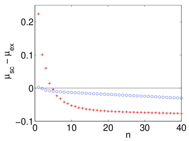
Figure 5: Solution of the NLSE for a harmonic potential: Error of the semiclassical calculation of the chemical potential $\mu_{sc}-\mu_{ex}$ in dependence of the quantum number $n$ for $g=1$ (blue circles) and $g=10$ (red crosses).

Figure 5 shows results for different quantum numbers $n$. The error of the semiclassical calculation, i.e. the difference of the semiclassical value for the chemical potential $\mu_{sc}$ and the numerically exact value $\mu_{ex}$ is plotted against the quantum number $n$ for $g=1$ and $g=10$. Except for very small values of $n$ and $g=10$, for which the reduction to the asymptotic form (7) is not valid, one obtains reasonable results for the semiclassical approximation.

The method introduced above can be extended to asymmetric trapping potentials. Then one has to construct solutions around the two classical turning points separately, which are matched at a ’mid-phase point’ [20]. In this spirit the restriction to symmetric or anti-symmetric solutions above is nothing but a matching of two solutions at the mid-phase point $x=0$.

In the linear case $g=0$ a mapping to a similar potential with two classical turning points, in fact the harmonic potential, avoids this matching procedure [21]. In the nonlinear case, however, the single-turning point equation $P_{II}$ has some advantages compared to the NLSE with a harmonic potential because the $P_{II}$ equation is free of movable branch points and connection formulae are well known.

5 Mapping to a constant potential

It is well-known that the free NLSE

$$\frac{{\rm d}^{2}\phi}{{\rm d}y^{2}}+2\nu\phi(y)-2g\phi(y)^{3}=0$$ (25)

has soliton solutions. Bright solitons are found for $\nu<0$ and $g<0$, given by

$$\phi(y)=\sqrt{2\nu/g}\,{\rm sech}\left(\sqrt{-2\nu}(y-y_{0})\right),$$ (26)

and dark solitons for $\nu<0$ and $g>0$ are given by

$$\phi(y)=\sqrt{\nu/g}\tanh\left(\sqrt{\nu}(y-y_{0})\right).$$ (27)

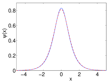
Figure 6: Bright soliton solution in a cosine-potential of strength $w=-0.2$ for $\mu=-1$. Numerically exact results (solid blue line) are compared to results from the mapping technique (dashed red line).

Using a mapping technique as in the previous section we explore the effects of a small additional cosine potential on these solitons. In fact we consider the NLSE

$$\frac{{\rm d}^{2}\psi}{{\rm d}x^{2}}+2(\mu-w\cos(x))\psi(x)-2g\psi(x)^{3}=0$$ (28)

Using again the ansatz (17) and following the lines of reasoning of section 4, one arrives at

$$\left(\frac{{\rm d}y}{{\rm d}x}\right)^{2}\left[2g\phi^{3}-2\nu\phi\right]+2(\mu-v\cos(x))\phi-2ga^{2}\left(\frac{{\rm d}y}{{\rm d}x}\right)^{-1}\phi^{3}=0$$ (29)

Again one chooses the scaling factor $a$ to minimize the difference of the nonlinear terms

$$\chi^{2}=\int_{-\infty}^{\infty}\left[g\left(\frac{{\rm d}y}{{\rm d}x}\right)^{2}-ga^{2}\left(\frac{{\rm d}y}{{\rm d}x}\right)^{-1}\right]^{2}\phi(y(x))^{6}\,{\rm d}x$$ (30)

and neglects them in equation (29) to arrive at the mapping equation

$$\left(\frac{{\rm d}y}{{\rm d}x}\right)^{2}=\frac{\mu-w\cos(x)}{\nu}$$ (31)

To ensure that the right-hand side is positive, one must always be in the classically allowed region ($\mu>w$, thus $\nu>0$) or the classically forbidden region ($\mu<-w$, thus $\nu<0$); values in the interval $\mu\in(-w,w)$ cannot be treated within this framework.

To show the validity of this method we calculate a bright soliton solution in a cosine lattice $V(x)=w\cos(x)$. Figure 6 shows the wavefunction calculated by the mapping method in comparison to the numerically exact solution. One observes a good agreement.

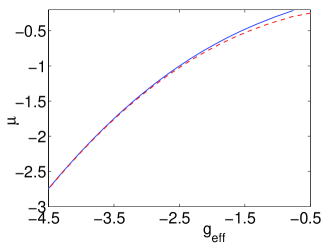
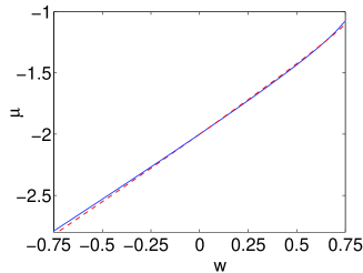
Figure 7: Shift of the chemical potential of a bright soliton in a cosine-potential in dependence of the nonlinearity $g_{\rm eff}$ for $w=-0.2$ (left) and in dependence of the potential strength $w$ for $g_{\rm eff}-4$ (right). Numerically exact results (solid blue line) are compared to results from the mapping technique (dashed red line).

Furthermore we calculate the dependence of the chemical potential potential $\mu$ of such a bright soliton on the nonlinarity $g_{\rm eff}$ for a fixed value of $w$ and on the potential strength $w$ for a fixed nonlinearity $g_{\rm eff}$. The results obtained by the mapping method and the numerically exact results are compared in figure 7. One observes a good agreement.

References

- [1] L. Pitaevskii and S. Stringari, Bose-Einstein Condensation, Oxford University Press, Oxford, 2003
- [2] L. D. Carr, C. W. Clark, and W. P. Reinhardt, Phys. Rev. A 62 (2000) 063610
- [3] L. D. Carr, C. W. Clark, and W. P. Reinhardt, Phys. Rev. A 62 (2000) 063611
- [4] D. Witthaut, S. Mossmann, and H. J. Korsch, J. Phys. A 38 (2005) 1777
- [5] D. Witthaut, K. Rapedius, and H. J. Korsch, preprint: cond–mat/0506645
- [6] B. T. Seaman, L. D. Carr, and M. J. Holland, Phys. Rev. A 71 (2005) 033622
- [7] J. C. Bronski, L. D. Carr, B. Deconinck, and J. N. Kutz, Phys. Rev. Lett. 86 (2001) 1402
- [8] V. V. Konotop and P. G. Kevrekidis, Phys. Rev. Lett. 91 (2003) 230402
- [9] T. Hyouguchi, S. Adachi, and M. Ueda, Phys. Rev. Lett. 88 (2002) 170404
- [10] T. Hyouguchi, R. Seto, M. Ueda, and S. Adachi, Annals of Physics 312 (2004) 177
- [11] M. Greiner, I. Bloch, O. Mandel, T. W. Hänsch, and T. Esslinger, Appl. Phys. B 73 (2001) 769
- [12] M. Olshanii, Phys. Rev. Lett. 81 (1998) 938
- [13] R. K. Dodd, J. C. Eilbeck, J. D. Gibbon, and H. C. Morris, Solitons and nonlinear wave equations, Academic Press, London, 1982
- [14] K. Iwasaki, H. Kimura, S. Shimomura, and M. Yoshida, From Gauss to Painlevé, A modern Theory of special Functions, Vieweg, Braunschweig, 1991
- [15] M. J. Ablowitz and P. A. Clarkson, Solitons, nonlinear evolution equations and inverse scattering, Cambridge University Press, Cambridge, 1991
- [16] M. J. Ablowitz and H. Segur, Phys. Rev. Lett. 38 (1977) 1103
- [17] H. Segur and M .J. Ablowitz, Physica D 3 (1981) 165
- [18] V. V. Nesvizhevsky, H. G. Börner, A. K. Petukhov, H. Abele, S. Baeßler, F. J. Ruess, T. Stöferle, A. Westphal, A. M. Gagarski, G. A. Petrov, and A. V. Strelkov, Nature 415 (2002) 297
- [19] R. D’Agosta and C. Presilla, Phys. Rev. A 65 (2002) 043609
- [20] H. H. Miller, J. Chem. Phys. 48 (1968) 464
- [21] M. V. Berry and K.E. Mount, Rep. Prog. Phys. 35 (1972) 315