Entanglement fidelity of quantum memories

Abstract

We introduce a figure of merit for a quantum memory which measures the preservation of entanglement between a qubit stored in and retrieved from the memory and an auxiliary qubit. We consider a general quantum memory system consisting of a medium of two level absorbers, with the qubit to be stored encoded in a single photon. We derive an analytic expression for our figure of merit taking into account Gaussian fluctuations in the Hamiltonian parameters, which, for example, model inhomogeneous broadening and storage time dephasing. Finally we specialize to the case of an atomic quantum memory where fluctuations arise predominantly from Doppler broadening and motional dephasing.

The ability to store flying qubits in a quantum memory (QM) is a fundamental component of many quantum communication schemes briegeletal ; duretal . Numerous possible methods for storing and retrieving qubits encoded in light pulses have been proposed fleischhauerlukin1 ; polzik ; kraus , and some of these proposals have recently been experimentally realized, achieving e.g. storage and retrieval of a single photon on demand chaneliere ; julsgaard , and entanglement between light and matter monroe ; polzik . Many promising candidate systems for QMs such as atomic ensembles lukin , arrays of quantum dots santori or NV centers in diamond kurtsiefer can often effectively be described as ensembles of $N$ two-level absorbers coupling to the incoming qubit. We consider two independent ensembles each storing one of the logical qubit states. The absorbers consist of two meta-stable internal states $\left|\,g\right\rangle$ and $\left|\,e\right\rangle$ as shown in Fig. 1(a), and a transition $\left|\,g\right\rangle\rightarrow\left|\,e\right\rangle$ is effected by the incoming photon in logical state $q$ via coupling $\Omega_{q}$. The states $\left|\,g\right\rangle$ and $\left|\,e\right\rangle$ are usually not directly connected optically, with this transition often being achieved via an intermediate state $\left|\,\mathrm{int}\right\rangle$ and additional control fields. For most of this paper details of such additional structure in the absorbing medium are not considered, and we assume that its effects on the properties of the absorbers can be subsumed into stochastic fluctuations of the coupling parameter $\Omega_{q}$. After a storage time $t_{s}$ another control field is used to retrieve the photonic qubit. Dephasing may take place in the memory during the storage time, which usually leads to different couplings when writing and reading the qubit.

Using these general assumptions and the notion of entanglement fidelity schumacher we derive a figure of merit $\cal F$ that measures how well a QM setup can preserve entanglement between a qubit undergoing the memory process (the memory qubit) and an auxiliary qubit. Our figure of merit $\cal F$ is different from commonly-used quality measures such as average fidelity $F_{A}$ for a pre-defined set of input qubit states hammerer . This captures the ability of a memory to recreate the initial state of the qubit, and is equal to $1$ if and only if the memory stores and retrieves every state perfectly. However, depending on the application of the QM, one might not necessarily be concerned with exactly preserving the quantum state of the qubit. The preservation of entanglement might be more desirable in some quantum information processing and quantum communication schemes ekert1 ; bennett , for example in a quantum repeater briegeletal ; duretal or in the cascaded generation of graph states raussendorf . The entanglement fidelity $\cal F$ also directly relates to the degree of violation of a Bell inequality by an EPR pair of photons, where one photon is stored and subsequently retrieved from the QM while the auxiliary qubit is directly detected as schematically shown in Fig. 1(b). The setup shown in Fig. 1(b) could thus be used to measure our figure of merit.

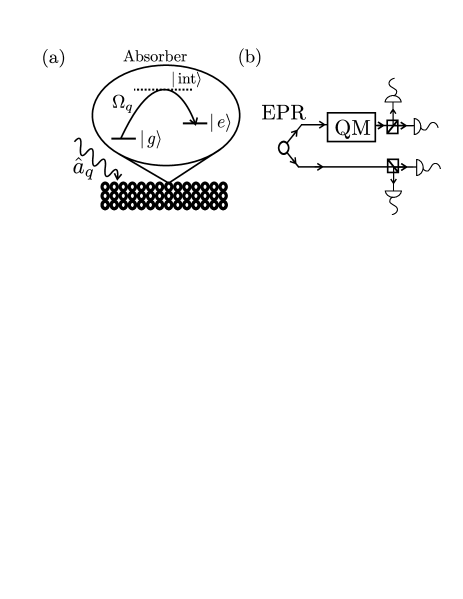
Figure 1: (a) General level structure of an absorber in a QM. A photon with annihilation operator $\hat{a}_{q}$ is incident on a medium of $N$ absorbers, and excites one absorber into state $\left|\,e\right\rangle$ via an intermediate state $\left|\,\mathrm{int}\right\rangle$. (b) Schematic experimental setup. We consider a photonic qubit entangled with an auxiliary qubit produced by an EPR source. The photonic qubit is stored in the memory, and the amount of entanglement that remains after storage is measured.

In the system outlined above the memory qubit is encoded in a subspace of the overall photon Hilbert space $\mathcal{H}_{A}$. The states of the memory and auxiliary qubits are denoted by $\left|\,0\right\rangle$ and $\left|\,1\right\rangle$. The Hilbert spaces of the auxiliary qubit and the medium are $\mathcal{H}_{B}$ and $\mathcal{H}_{C}$ respectively. The system has initial state $\hat{\rho}_{0}=\left|\,\phi_{0}\right\rangle\left\langle\phi_{0}\,\right|\otimes\hat{\rho}_{C}$, where $\left|\,\phi_{0}\right\rangle\in\mathcal{H}_{A}\otimes\mathcal{H}_{B}$ and $\hat{\rho}_{C}$ is the initial density operator of the medium. We assume that the absorbers are not correlated initially and characterize a QM as a quantum operation $\Lambda_{M}$ that acts on the photon as follows

$$\Lambda_{M}\otimes\mathbb{I}:\left|\,\phi_{0}\right\rangle\left\langle\phi_{0}\,\right|\rightarrow\mathrm{tr}_{C}\left[\hat{\mathcal{L}}(\hat{\rho}_{0})\right]\mbox{,}$$ (1)

where $\hat{\mathcal{L}}$ is a Liouvillian operating on states in $\mathcal{H}_{A}\otimes\mathcal{H}_{C}$, and $\mathbb{I}$ is the identity operator on states in $\mathcal{H}_{B}$. We note that in the work of A. K. Ekert et al. ekert a quantum channel for qubits $\Lambda$ is characterized by considering the action of the operator $\Lambda\otimes\mathbb{I}$ on two qubit states. The superoperator $\Lambda_{M}\otimes\mathbb{I}$ preserves entanglement for all two-qubit states only if $\Lambda_{M}$ is unitary (the converse is well known plenio ). This can be seen by using a Kraus decomposition of $\Lambda_{M}$. We find that for at least one initial two-qubit state $\left|\,\phi_{e}\right\rangle$ the application of a non-unitary $\Lambda_{M}$ will result in a mixed state. Purification of $(\Lambda_{M}\otimes\mathbb{I})(\left|\,\phi_{e}\right\rangle\left\langle\phi_{e}\,\right|)$ results in the introduction of an extra ancillary system, with which the memory qubit is entangled. By monogamy of entanglement wootters ; koashi ; bruss , the entanglement between the memory and auxiliary qubits decreases.

Motivated by these observations we write a QM entanglement fidelity as follows

$$\mathcal{F}(\Lambda_{M})=\min_{\left|\,\phi_{0}\right\rangle}\left\{\left\langle\phi_{0}\,\right|\hat{U}_{M}^{\dagger}\left[(\Lambda_{M}\otimes\mathbb{I})(\left|\,\phi_{0}\right\rangle\left\langle\phi_{0}\,\right|)\right]\hat{U}_{M}\left|\,\phi_{0}\right\rangle\right\}\mbox{.}$$ (2)

The quantity inside the braces is the entanglement fidelity schumacher for the process $\Lambda_{M}$ applied to the state $\mathrm{tr}_{B}[\left|\,\phi_{0}\right\rangle\left\langle\phi_{0}\,\right|]$ ($\mathrm{tr}_{B}$ denotes the partial trace over $\mathcal{H}_{B}$). The entanglement fidelity was introduced as a measure to characterize how well entanglement is preserved by such a process in schumacher , and detailed discussions of its properties can be found in schumacher ; nielsen ; kretschmann . Since the standard definition of entanglement fidelity nielsenchuang measures preservation of state as well as entanglement we include a unitary $\hat{U}_{M}$, which acts on $\mathcal{H}_{A}$, to allow for evolution of the photon that would not decrease the entanglement present. This unitary is chosen to maximize $\cal F$, and thus describes an optimized storage process to which $\Lambda_{M}$ is compared in the same way that gate fidelity nielsenchuang measures the success of a quantum gate. We also minimize over all pure two-qubit input states so that $\mathcal{F}$ is a property only of the QM that uses the worst-case scenario as a measure of its success. The QM $\Lambda_{M}$ (and hence the Liouvillian $\hat{\mathcal{L}}$) consists of a read-in process, a period of storage, and a read-out process that retrieves the photon on demand a time $t_{s}$ after read-in. Note that more sophisticated choices for $\hat{U}_{M}$ conditional on the outcome of measurements on the state of the QM after retrieving the photon might enable further improvement of $\cal F$. However, such schemes are difficult to realize experimentally and are not considered in this paper. Thus if $\mathcal{F}=1$ we have that $\Lambda_{M}$ preserves entanglement between the qubits, but the final and initial states of the photon may be deterministically different. The representation of the QM with $\Lambda_{M}$ illustrates that for ${\cal F}<1$ the memory process will not be unitary.

We now consider the photon and its interaction with the ensemble of absorbers. We define the annihilation operator $\hat{a}_{q}$ for the photon in state $\left|\,\underline{q}\right\rangle=\hat{a}_{q}^{\dagger}\left|\,\mathrm{vac}\right\rangle$, where $\left|\,\mathrm{vac}\right\rangle$ represents the vacuum state and $q=0,1$ denotes the logical state of the qubit (the underline distinguishes states in $\mathcal{H}_{A}$ from memory qubit states). This annihilation operator can be written as

$$\hat{a}_{q}=\int\mathrm{d}\mathbf{k}g_{q}(\mathbf{k})\hat{a}_{\mathbf{k},\lambda_{q}}\mbox{,}$$ (3)

where $\hat{a}_{\mathbf{k},\lambda_{q}}$ destroys a photon with polarization $\lambda_{q}$ and wavevector $\mathbf{k}$. The mode functions $g_{q}(\mathbf{k})$ are normalized, $[\hat{a}_{q},\hat{a}_{q^{\prime}}^{\dagger}]=\delta_{qq^{\prime}}$ and for simplicity we have assumed that each logical state has an associated single polarization $\lambda_{q}$. The absorbers are initially in the collective state $\left|\,G\right\rangle=\left|\,g_{1},\dots,g_{N}\right\rangle$, and are assumed to coherently couple to the photon during the whole of the read-in and read-out processes. The Hamiltonian for the read-in interaction between the photon in state $\left|\,\underline{q}\right\rangle$ and the $j^{\mathrm{th}}$ absorber is given by $\hat{H}_{q}^{(j)}=(\Omega_{q,j}\hat{a}_{q,j}\hat{\sigma}_{eg}^{(j)}+\mathrm{H.c.})$, where $\hat{\sigma}^{(j)}_{eg}=\left|\,e\right\rangle_{j}\left\langle g\,\right|$. During storage each absorber evolves according to the Hamiltonian $\hat{H}_{S,q}^{(j)}=s_{q,j}(t)\hat{\sigma}_{ee}^{(j)}$, with $s_{q,j}(t)$ some time-dependent detuning. The read-out interaction of the photon in logical state $\left|\,q\right\rangle$ with the absorber is modeled by the Hamiltonian $\hat{\tilde{H}}_{q}^{(j)}=(\tilde{\Omega}_{q,j}\hat{b}_{q,j}\hat{\sigma}_{eg}^{(j)}+\mathrm{H.c.})$, with couplings $\tilde{\Omega}_{q,j}$. The dependence of the operators $\hat{a}_{q,j}$ and $\hat{b}_{q,j}$ on the absorber reflects the fact that due to motion each absorber will in general couple to a slightly different mode. We assume that an appropriate choice of control field can restrict this effect to a phase $\delta_{q,j}^{(a)}$, so that $\hat{a}_{q,j}=\hat{a}_{q}\exp{(i\delta_{q,j}^{(a)})}$, and similarly for the output photon mode $\hat{b}_{q,j}=\hat{b}_{q}\exp{(i\delta_{q,j}^{(b)})}$. The read-in and read-out processes are assumed to require a time $t_{p}$ each. In general the couplings $\Omega_{q,j}$ and $\tilde{\Omega}_{q,j}$ will depend on time $t$. In the following we assume a simple time dependence where the magnitude of the read-in (read-out) coupling is switched on to a constant value for the time $t_{p}$ that maximizes storage (retrieval), then switched off. For simplicity we also let $|\Omega_{q,j}|=|\tilde{\Omega}_{q,j}|\forall j$ – the generalization to different couplings is straightforward. Inhomogeneous broadening can furthermore lead to phases linearly increasing with time, and during storage some additional dephasing can occur. As a result of these assumptions we write $\Omega_{q,j}=\kappa_{q,j}e^{\mathrm{i}(K_{q,j}t)}$ and $\tilde{\Omega}_{q,j}=\kappa_{q,j}e^{\mathrm{i}[M_{q,j}t+f_{q,j}(t_{s})]}$, where $f_{q,j}(t_{s})$ appears as a result of eliminating $\hat{H}_{S,q}^{(j)}$ from the dynamics. The parameters $\kappa_{q,j}$, $K_{q,j}$, $M_{q,j}$, $\delta_{q,j}^{(a)}$, $\delta_{q,j}^{(b)}$ and $f_{q,j}(t_{s})$ are all assumed to be real normally-distributed stochastic variables with respect to the storage medium. For instance $K_{q,j}$ is broadened around a mean value $\bar{K}_{q}$ by a width $w_{K,q}$ and so on.

To obtain an analytical expression for $\mathcal{F}$, we first note that if $K_{q,j}=\bar{K}_{q}\forall j$ the system reduces to a two-level problem, and the evolution during read-in can be solved exactly. To this end we rewrite the read-in Hamiltonian

$$\hat{H}_{q}^{(j)}=\kappa_{q,j}[e^{\mathrm{i}\bar{K}_{q}t}+e^{\mathrm{i}\bar{K}_{q}t}(e^{\mathrm{i}\delta_{q,j}^{(K)}t}-1)]\hat{a}_{q,j}\hat{\sigma}_{eg}^{(j)}+\mathrm{H.c.}$$

and treat the term containing the fluctuation $\delta_{q,j}^{(K)}$ in $K_{q}$ perturbatively up to second order, and similarly for $\hat{\tilde{H}}_{q}^{(j)}$. Since any mean broadening could be corrected for, we assume that $\bar{K}_{q}=\bar{M}_{q}=0$ for simplicity. The general initial normalized photon and auxiliary qubit state can be written as $\left|\,\phi_{0}\right\rangle=\alpha\left|\,\underline{0}0\right\rangle+\beta\left|\,\underline{0}1\right\rangle+\gamma\left|\,\underline{1}0\right\rangle+\eta\left|\,\underline{1}1\right\rangle$. For each component of $\left|\,\phi_{0}\right\rangle$ the evolution operator $\hat{U}$ according to $\sum_{j}\hat{H}_{q}^{(j)}$ and $\sum_{j}\hat{\tilde{H}}_{q}^{(j)}$ can be used to calculate the final wavefunction of the system at time $t_{f}=t_{s}+2t_{p}$. Averaging over the ensemble similarly to DCZ allows us to rewrite Eq. (1) as

$$\Lambda_{M}\otimes\mathbb{I}:\left|\,\phi_{0}\right\rangle\left\langle\phi_{0}\,\right|\rightarrow\left\langle\left\langle\hat{U}(\left|\,\phi_{0}\right\rangle\left\langle\phi_{0}\,\right|\otimes\left|\,G\right\rangle\left\langle G\,\right|)\hat{U}^{\dagger}\right\rangle\right\rangle\mbox{,}$$ (4)

where $\left\langle\left\langle\dots\right\rangle\right\rangle$ denotes averaging over the stochastic Hamiltonian variables then tracing out the memory. Since $\left|\,\phi_{0}\right\rangle$ is normalized $\cal F$ can be calculated by minimizing over a single parameter $X=\left|\alpha\right|^{2}+\left|\beta\right|^{2}$ in Eq. (2). This results in

$${\cal F} = \left\{X_{0}^{2}\big{\langle}\big{\langle}\left|b_{0}\right|^{2}\big{\rangle}\big{\rangle}+2X_{0}(1-X_{0})\mathrm{Re}\left\{\big{\langle}\big{\langle}b_{0}b_{1}^{*}\big{\rangle}\big{\rangle}\right\}\right.$$ (5)

$$\left.+(1-X_{0})^{2}\big{\langle}\big{\langle}\left|b_{1}\right|^{2}\big{\rangle}\big{\rangle}\right\}\mbox{,}$$

where $X_{0}$ is the value of $X$ that achieves the minimization in Eq. (2), and $b_{q}$ is the amplitude of the final output photon in logical state $q$. Differentiating $\mathcal{F}$ with respect to $X$ gives a minimum of

$$X_{0}=\frac{\big{\langle}\big{\langle}\left|b_{1}\right|^{2}\big{\rangle}\big{\rangle}-\mathrm{Re}\left\{\big{\langle}\big{\langle}b_{0}b_{1}^{*}\big{\rangle}\big{\rangle}\right\}}{\big{\langle}\big{\langle}\left|b_{0}\right|^{2}\big{\rangle}\big{\rangle}-2\mathrm{Re}\left\{\big{\langle}\big{\langle}b_{0}b_{1}^{*}\big{\rangle}\big{\rangle}\right\}+\big{\langle}\big{\langle}\left|b_{1}\right|^{2}\big{\rangle}\big{\rangle}}\mbox{,}$$ (6)

but if this value lies outside $[0,1]$ then $X_{0}=0$ or $1$. Applying second-order perturbation theory to the read-in and read-out processes as previously described gives

$$\big{\langle}\big{\langle}\left|b_{q}\right|^{2}\big{\rangle}\big{\rangle}=\bigg{[}1-\frac{\Theta(w_{K,q}^{2}+w_{M,q}^{2})}{8N(\bar{\kappa}_{q}^{2}+w_{\kappa,q}^{2})}\bigg{]}\bigg{[}\frac{1}{N}+$$

$$\qquad+\frac{(N-1)}{N(1+\tilde{w}_{\kappa,q}^{2})^{2}}e^{-(w_{a,q}^{2}+w_{b,q}^{2}+w_{f,q}(t_{s})^{2})}\bigg{]}\mbox{,}$$ (7)

$$\mathrm{Re}\left\{\big{\langle}\big{\langle}b_{0}b_{1}^{*}\big{\rangle}\big{\rangle}\right\}=\prod_{q=0,1}\bigg{[}\frac{e^{-(w_{a,q}^{2}+w_{b,q}^{2}+w_{f,q}(t_{s})^{2})/2}}{1+\tilde{w}_{\kappa,q}^{2}}\bigg{]}$$

$$\qquad\times\bigg{[}1-\sum_{q=0,1}\frac{(4+\pi^{2})\Theta(w_{K,q}^{2}+w_{M,q}^{2})}{64N^{2}(\bar{\kappa}_{q}^{2}+w_{\kappa,q}^{2})}\bigg{]}\mbox{,}$$ (8)

where $\tilde{w}_{\kappa,q}=w_{\kappa,q}/\overline{\kappa}_{q}$, and $\Theta=(1+6\tilde{w}_{\kappa,q}^{2}+3\tilde{w}_{\kappa,q}^{4})/(1+\tilde{w}_{\kappa,q}^{2})^{2}$. We see that $\mathcal{F}$ decreases exponentially in $w_{a,q}$, $w_{b,q}$ and $w_{f,q}(t_{s})$, and also decreases as both $\tilde{w}_{\kappa,q}$ and $w_{x,q}^{2}/\overline{\kappa_{q}^{2}}$ increase ($x=K,M$). Due to the factors of $1/N$ appearing in these latter terms, it is the exponential terms that will dominate for large $N$. Let us also note that to obtain maximum absorption and emission we set $t_{p}=\pi/2(\overline{\kappa_{q}^{2}}N)^{1/2}$, so the terms containing $w_{x,q}$ could alternatively be seen to depend quadratically on $t_{p}$. Finally, we observe that sufficient conditions for $\mathcal{F}\lesssim 1$ are that $w_{a,q},w_{b,q},w_{f,q}(t_{s})\ll 1$ and $\omega_{K,q},\omega_{M,q}\ll\overline{\kappa^{2}}$, with the latter becoming less important as $N\rightarrow\infty$.

The value of $X_{0}$ represents the class of states that achieve the minimum required in Eq. (2). To illustrate this let us consider some special cases. (i) If the states $\left|\,\underline{0}\right\rangle$ and $\left|\,\underline{1}\right\rangle$ of the photon are absorbed and emitted in the same way ($b_{0}=b_{1}$), then evaluating $X_{0}$ gives an indeterminate answer, reflecting the fact that $\mathcal{F}$ is minimized by several choices of $\left|\,\phi_{0}\right\rangle$. Evaluation of $\mathcal{F}$ in this situation gives a value $\mathcal{F}=\big{\langle}\big{\langle}\left|b_{0}\right|^{2}\big{\rangle}\big{\rangle}$. (ii) If state $\left|\,\underline{1}\right\rangle$ is perfectly stored, but state $\left|\,\underline{0}\right\rangle$ is not stored at all, then $b_{0}=0$, $X_{0}=1$, and $\mathcal{F}=0$. We also compare our measure with the previously-defined fidelity $F_{A}$. If entanglement is preserved i.e. ${\cal F}=1$ then $F_{A}=1$ if and only if the output photon has the same mode function as the input photon. In the case where the photon is stored and emitted with $100\%$ probability, but becomes completely decorrelated with the auxiliary qubit $F_{A}$ could vary between $0$ and $1$ depending on the spatial mode function of the output photon, but ${\cal F}=1/2$.

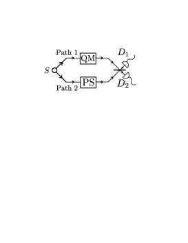
Figure 2: Experimental method of measuring $\cal F$ requiring storage of one logical state only. A source $S$ produces a separable pair of photons, so that photon 1 is stored in the QM and photon 2 enters the pulse shaper (PS). The photons interfere at a beam splitter (the PS includes a time delay), and coincidence measurements at detectors $D_{1}$ and $D_{2}$ are made.

We now describe an experimental setup (shown in Fig. 2) that, assuming case (i) above holds, would allow us to measure $\mathcal{F}$. After read-out but before the beam splitter (BS) the state of the photons will be $\hat{\rho}_{\mathrm{in}}=\hat{a}_{PS}^{\dagger}\bigg{\{}\sum_{m}[p_{m}(\hat{b}_{m}^{\mathrm{out}})^{\dagger}\left|\,\mathrm{vac}\right\rangle\left\langle\mathrm{vac}\,\right|\hat{b}_{m}^{\mathrm{out}}]+p_{0}\left|\,\mathrm{vac}\right\rangle\left\langle\mathrm{vac}\,\right|\bigg{\}}\hat{a}_{PS}$, where $\left|\,\mathrm{vac}\right\rangle$ denotes the vacuum, $\hat{a}_{PS}$ is the annihilation operator for the mode of photon $2$ after the pulse shaper (PS), and $\left\{\hat{b}_{m}^{\mathrm{out}}\right\}$ with $m\geq 1$ is the set of annihilation operators corresponding to the eigenmodes of the state of photon $1$. The eigenvalues are in descending order $p_{1}\geq p_{2}\geq\dots$ and $p_{0}$ is the probability of not retrieving the photon on demand. Noting that most detectors cannot resolve photon number, the probability of obtaining a click in one of the detectors $D_{j}$ ($j=1,2$) is $P_{j}=\sum_{m=1}^{\infty}p_{m}(1+{\cal O}_{m})/4+p_{0}/2$, and of a detection in both $D_{1}$ and $D_{2}$ is $P_{12}=\sum_{m=1}^{\infty}p_{m}(1-{\cal O}_{m})/2$, where ${\cal O}_{m}=|\left\langle\rm vac\,\right|\hat{a}_{PS}(\hat{b}_{m}^{\mathrm{out}})^{\dagger}\left|\,\mathrm{vac}\right\rangle|^{2}$ is the overlap of the field modes after the BS. Both the minimum value of $P_{12}$ and the maximum value of $P_{1}+P_{2}$ are obtained when $\hat{a}_{PS}=\hat{b}_{1}^{\mathrm{out}}$ i.e. when the mode of photon $2$ is precisely the dominant mode of photon $1$ and for this setting $p_{0}+p_{1}=P_{1}+P_{2}-P_{12}$. Hence by tuning the PS the dominant mode of the memory photon can be found experimentally. This tuning then corresponds to the $\hat{U}_{M}$ that maximizes $\mathcal{F}$ as in Eq. (2). We can then deduce $p_{1}=\big{\langle}\big{\langle}\left|b_{0}\right|^{2}\big{\rangle}\big{\rangle}$ by removing the beam splitter and measuring the probability of the memory photon not being re-emitted on demand. Therefore $\mathcal{F}$ can be deduced.

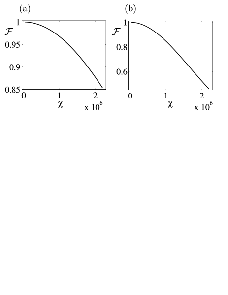
Figure 3: The entanglement fidelity of a Raman QM with (a) $\zeta=4.49\times 10^{-14}$, (b) $\zeta=2.25\times 10^{-13}$. In both cases the photon bandwidth $\delta_{p}=0.1\Delta$, with $\Delta=10^{13}\mathrm{s}^{-1}$. The atomic level splittings used are $\left|\,g\right\rangle\rightarrow\left|\,\mathrm{int}\right\rangle=5\times 10^{15}\mathrm{s}^{-1}$ and $\left|\,e\right\rangle\rightarrow\left|\,\mathrm{int}\right\rangle=3.5\times 10^{15}\mathrm{s}^{-1}$, and the ensemble consisted of $N=10^{8}$ atoms.

We conclude our analysis by applying the fidelity measure $\mathcal{F}$ to a specific memory setup. We determine $\mathcal{F}$ for a QM for one single photon state based on off-resonant stimulated Raman scattering in an ensemble of $\Lambda$-atoms nunn . The atoms each have mass $M$ and temperature $T$, and have the same internal level structure as the general absorbers considered in Fig. 1(a). The photon is incident on the ensemble and excites the $\left|\,g\right\rangle\rightarrow\left|\,\mathrm{int}\right\rangle$ transition. A control field drives $\left|\,\mathrm{int}\right\rangle\leftrightarrow\left|\,e\right\rangle$ and stores the photon as a collective excitation in the ensemble. The probe and control fields are assumed to co-propagate with carrier wavevectors of magnitude $k_{p}$ and $k_{c}$ respectively. Retrieval of the photon is achieved by applying another control field a time $t_{s}$ after read-in. We assume that the probe and control fields are both far-detuned (detuning $\Delta$) from level $\left|\,\mathrm{int}\right\rangle$, so this state can be adiabatically eliminated giving a medium consisting effectively of two-level atoms. Therefore the main source of stochastic variation in the coupling of the atoms to the photon arises from the atomic motion, which we treat semiclassically assuming a Boltzmann distribution for atomic velocity components $v_{j}$ in the direction of the field propagation. This leads to $K_{q,j}=M_{q,j}=v_{j}\omega_{c}/c$, $f_{q,j}(t_{s})=\chi v_{j}/c$ and widths given by $w_{K,q}=w_{M,q}=\omega_{c}\zeta^{1/2}$, $w_{f,q}=\chi\zeta^{1/2}$, where $c$ is the speed of light, $\zeta=k_{B}T/Mc^{2}$, $\chi=(k_{p}-k_{c})ct_{s}$, and $\omega_{c}=ck_{c}$. In this scheme $f_{q,j}(t_{s})$ originates from the motion of the atoms during the storage time and $K_{q,j}$ and $M_{q,j}$ arise from the Doppler-shifting of the field frequencies. The parameter $\kappa_{q}=\kappa$ is defined by the couplings of the photon and control fields to the atoms, and is assumed to be a constant.

The amplitude of the final photon state can be calculated as for the general case, which upon substitution into Eq. (5) yields the following expression for $\mathcal{F}$ up to $N^{-2}$,

$$\mathcal{F}=e^{-\chi^{2}\zeta/2}(1-\chi^{2}\zeta)\bigg{[}e^{-\chi^{2}\zeta/2}(1-\chi^{2}\zeta)-\frac{3\zeta\omega_{c}^{2}}{2\kappa^{2}N^{2}}\bigg{]}.$$ (9)

We see that the two main contributions to the decrease in $\mathcal{F}$ are the Doppler broadening terms, which are quadratic in the ratio $\omega_{c}\sqrt{\zeta}/\kappa$, and the storage time dephasing terms, which depend on $\chi^{2}\zeta$. This observation results in the requirement that $\chi\sqrt{\zeta}\ll 1$ in order to achieve $\mathcal{F}\lesssim 1$ for $N\gg 1$. Fig. 3 shows the entanglement fidelity of the Raman quantum memory for two different values of $\zeta$, and the expected decrease in $\mathcal{F}$ with increasing $\chi$ is observed.

In summary we have introduced a figure of merit $\mathcal{F}$ for a general QM based on gate fidelity and derived an analytical expression for it. Our calculations took into account stochastic fluctuations in the coupling parameters whose origin might vary for different QM schemes. We concluded by applying our formalism to a specific atomic quantum memory.

References

(1) H. J. Briegel et al., Phys. Rev. Lett. 81,
5932 (1998).
(2) W. Dür et al., Phys. Rev. A 59, 169 (1999).
(3) M. Fleischhauer and M. D. Lukin, Phys. Rev. A 65, 022314 (2002).
(4) C. A. Muschik et al., Phys. Rev. A 73, 062329 (2006).
(5) B. Kraus et al., Phys. Rev. A 73,
020302(R) (2006).
(6) T. Chanelière et al., Nature 438, 833 (2005).
(7) B. Julsgaard et al., Nature 432, 482 (2004).
(8) B. Blinov et al., Nature 428, 153 (2004).
(9) M. D. Lukin, Rev. Mod. Phys. 75, 457-472 (2003).
(10) C Santori et al., Nature 419, 594
(2002).
(11) C. Kurtsiefer et al., Phys. Rev. Lett. 85, 290 (2000).
(12) B. Schumacher, Phys. Rev. A 54, 2614
(1996).
(13) K. Hammerer et al., Phys. Rev. Lett. 94, 150503
(2005).
(14) A. K. Ekert, Phys. Rev. Lett. 67, 661 (1991).
(15) C. H. Bennett et al., Phys. Rev. Lett 70, 1895 (1993).
(16) R. Raussendorf and H.- J. Briegel, Phys. Rev. Lett. 86, 5188 (2001).
(17) A. K. Ekert et al.,
Phys. Rev. Lett 88, 217901 (2002).
(18) M. B. Plenio and S. Virmani, e-print arxiv/quant-ph/0504163 (2005).
(19) V. Coffman, J. Kundu, and W. K. Wootters, Phys. Rev. A, 61, 052306 (2000).
(20) M. Koashi and A. Winter, Phys. Rev. A 69, 022309 (2004).
(21) D. Bruß, Phys. Rev. A 60, 4344 (1999).
(22) M. A. Nielsen, eprint quant-ph/9606012 (1996).
(23) D. Kretschmann and R. F. Werner, New
J. Phys., 6, 26 (2004).
(24) M. A. Nielsen and I. L. Chuang, Quantum Information and Computation, Cambridge Univ.
Press (2000).
(25) L. M. Duan, J. I. Cirac and P. Zoller, Phys. Rev. A
66, 023818 (2002).
(26) J. Nunn et al., eprint arxiv/quant-ph/0603268 (2006).