Spectral statistics for scaling quantum graphs

Abstract

The explicit solution to the spectral problem of quantum graphs is used to obtain the exact distributions of several spectral statistics, such as the oscillations of the quantum momentum eigenvalues around the average, $\delta k_{n}=k_{n}-\bar{k}_{n}$, and the nearest neighbor separations, $s_{n}=k_{n}-k_{n-1}$.

I Introduction

Understanding statistical properties of the quantum spectra produced by the classically nonintegrable systems is one of the most fundamental problems of quantum chaos theory. According to the Random Matrix Theory (RMT), the statistics of the spectral fluctuations is universal, and reflects only the general symmetry properties of system BGS . The universality of the RMT approach and its ability to produce specific predictions are particularly valuable since the spectra of the systems to which it is applied are typically out of reach for direct analytical studies. On the other hand, understanding how the RMT distributions themselves emerge from the phase space structures used by semiclassical spectral theories, such as the periodic orbit theory, is a matter of intense research. There has been a number of publications Bogomolny dedicated to computing spectral statistics that are accessible via periodic orbit expansion for the density of states. This analysis was particularly complete for the quantum graphs Gaspard ; QGT , which are simple and convenient models of quantum chaos.

As a reminder, quantum graphs consist of a quantum particle moving on a quasi one-dimensional network with $B$ bonds and $V$ vertexes. In the limit $\hbar=0$, these systems produce a nonintegrable (mixing) classical counterpart - a classical particle moving on the same network, scattering randomly on its vertexes. Despite the apparent simplicity such system, its classical behavior exhibits many familiar features of multidimensional deterministic chaotic systems Gaspard , which is clearly manifested in quantum regime. Numerical investigations of the quantum graph spectra QGT show that the spectral distributions of sufficiently complicated networks are closely approximated by the RMT Wignerian distributions. On the other hand, periodic orbit theory for quantum graphs yields exact harmonic expansions for the density of states, spectral staircase, quantum and classical zeta functions, etc. Moreover, as shown recently in Fabula , the periodic orbit theory for the quantum graphs can be “localized” - it is possible to obtain the harmonic series expansion representation for the individual eigenvalues of the energy or of the momentum, $k_{n}=k(n)$, as a global function of the index $n$. Hence, despite classical nonintegrability the spectral problem for quantum networks is exactly solvable within the periodic orbit theory approach. This fact provides an interesting opportunity to obtain analytically several new spectral statistics in terms of the periodic orbit theory, which is the main subject of this Letter.

II Spectral distributions for regular quantum graphs

In the simplest case of the so called regular graphs Prima ; Stanza the individual momentum eigenvalues can be expanded into a periodic orbit series,

$$k_{n}=\frac{\pi}{L_{0}}n-\frac{2}{L_{0}}\sum_{p}\frac{A_{p}}{\omega_{p}}\sin\left(\frac{\omega_{p}}{2}\right)\sin\left(\omega_{p}n\right).$$ (1)

Here $L_{0}$ is the total action length of the graph, $A_{p}$ is the weight factor of a periodic orbit $p$, which is a function of the scattering coefficients at the graph vertexes Prima ; Stanza . The frequency $\omega_{p}=\pi\left(m_{p}^{1}L_{1}+...+m_{p}^{B}L_{B}\right)/L_{0}$, is defined by the numbers of times, $m^{i}_{p}$, the orbit $p$ passes over the bond $i$. As shown in Stanza ; Fabula , the series in (1) is convergent and bounded by $\pi/L_{0}$, so the values $k_{n}$ are locked within a sequence of periodic cells. The first term in (1) gives the average (Weyl) behavior of the eigenvalue $\bar{k}_{n}$ and the subsequent periodic orbit sum describes the fluctuations $\delta^{(0)}_{n}=L_{0}\left(k_{n}-\bar{k}_{n}\right)/\pi$ around the average.

The transition from the exact formula (1) to statistical description of $\delta^{(0)}_{n}$s can be made based on the well known fact from the analytical number theory Karatsuba that the sequence of the remainders $x_{n}=\left[\alpha n\right]_{\mathop{\rm mod}1}$, $n=1,2,...$, for any irrational number - $\alpha$ is uniformly distributed over the interval $x\in\left[0,1\right]$. Assuming the generic case in which every $\Omega_{i}=L_{i}/L_{0}$ is an irrational number, it is clear that parsing through the spectral sequence $k_{1}$, $k_{2}$, …, $k_{n}$,…, will generate a sequence of random phases in (1), defined via the combinations

$$x_{i}=\left[\pi\Omega_{i}n\right]_{\mathop{\rm mod}2\pi},$$ (2)

that are uniformly distributed in the interval $[0,2\pi]$. Hence, the deviations of the eigenvalues from the average, $\delta^{(0)}_{n}$, are statistically described by a series of random inputs

$$\delta^{(0)}_{x}=-\frac{2}{\pi}\sum_{p}\frac{A_{p}}{\omega_{p}}\sin\left(\frac{\omega_{p}}{2}\right)\sin\left(\vec{m}_{p}\vec{x}\right),$$ (3)

where $\vec{x}=\left(x_{1},...,x_{B}\right)$, which has the same structure as the periodic orbit sum (1) (see Fig. 1).

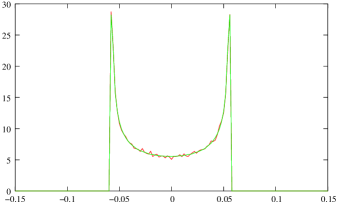
Figure 1: The histogram of the spectral fluctuations for the simplest regular two bond star graph obtained from the exact expansion (1) (shown in red), compared to the distribution obtained from (3) using the orbits that include up to 6 scattering events (shown in blue).

The distribution of $\delta$’s can then be obtained as

$$P^{(0)}_{\delta}(\delta^{(0)})=\int_{0}^{2\pi}\delta\left(\delta^{(0)}+\sum_{p}C^{(0)}_{p}\sin\left(\vec{m}_{p}\vec{x}\right)\right)dx$$ (4)

where $C_{p}^{(0)}=\frac{2A_{p}}{\pi\omega_{p}}\sin\frac{\omega_{p}}{2}$ and $dx=\prod_{i}\frac{dx_{i}}{2\pi}$. Using the exponential representation of the $\delta$ - functional, one finds that

$$P^{(0)}_{\delta}\left(\delta^{(0)}\right)=\int dk\,e^{ik\delta^{(0)}}F^{(0)}_{\delta}(k),$$ (5)

where

$$F^{(0)}_{\delta}(k)=\int_{0}^{2\pi}e^{ik\sum_{p}C_{p}^{(0)}\sin\left(\vec{m}_{p}\vec{x}\right)}\prod_{i}dx$$ (6)

is the characteristic function of the distribution. As in the case of the series expansion for $k_{n}$, a finite order ($l$th) approximation to the exact result in (5) is obtained by considering only the orbits that involve a particular number ($l$) of vertex scatterings Prima ; Stanza .

Similarly, for the spacings between two eigenvalues, $s^{(0)}_{n,m}=k_{n+m}-k_{n}$, the periodic orbit expansion,

$$s_{n,m}^{(0)}=\frac{\pi}{L_{0}}m-\sum_{p}D_{p,m}^{(0)}\cos\left(\omega_{p}\left(n-\frac{m}{2}\right)\right),$$ (7)

where $D_{p,m}^{(0)}=\frac{4}{L_{0}}\frac{A_{p}^{(0)}}{\omega_{p}}\sin\left(\frac{\omega_{p}}{2}\right)\sin\left(\frac{\omega_{p}m}{2}\right)$, yields the distribution $P_{s_{m}}^{(0)}$ of the type (5), where now

$$F^{(0)}_{s_{m}}(k)=\int_{0}^{2\pi}e^{ik\sum_{p}D_{p,m}^{(0)}\sin\left(\vec{m}_{p}\vec{x}-\frac{\omega_{p}m}{2}\right)}dx$$ (8)

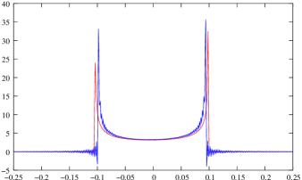
Figure 2: The histogram of the nearest neighbor separations for the regular two bond star graph obtained via direct numerical solution of the spectral equation (shown in red), compared to the distribution obtained from (8) (shown in blue). To emphasize the connection with Fig. 1, the graph is scaled and shifted along the abscissa by $\pi/L_{0}$.

Note, that despite the complete nonintegrability of the underlying classical system Gaspard , the statistics of the spectral fluctuations of certain (e.g. some regular) quantum graphs is not described by the RMT and so the shapes of their probability distributions deviate noticeably from the familiar Wignerian profiles (Fig. 2).

All the above distributions are exact and depend explicitly on the specific graph parameters - the vertex scattering coefficients and the periodic orbit set.

III Spectral hierarchy method

As shown in Fabula , a generic quantum graph systems is irregular. The idea of producing the statistical distribution profiles for irregular quantum graphs is based on three key properties of the spectral determinant $\Delta(k)$ Fabula , briefly outlined below. First, its roots as well as the roots of all of its derivatives are real. Secondly, there is exactly one root of $\Delta^{(j)}(k)$ between every two neighboring roots of $\Delta^{(j+1)}(k)$ Levin . This implies that the zeroes of $\Delta(k)$ can be bootstrapped by the zeroes of $\Delta^{\prime}(k)$, while the latter sequence can be bootstrapped by the roots of $\Delta^{\prime\prime}(k)$ and so on (Fig. 3). Hence, there exists a hierarchy of almost periodic sequences, $\hat{k}_{n}^{(j)}$, $j=0,1,...$, $\Delta^{(j)}\left(\hat{k}_{n}^{(j)}\right)=0$, such that $\hat{k}_{n-1}^{(j)}<\hat{k}_{n}^{(j-1)}<\hat{k}_{n}^{(j)}$ and

$$\hat{k}_{n}^{(j)}=\frac{\pi}{L_{0}}\left(n+\delta_{n}^{{}^{(j)}}\right).$$ (9)

Lastly, the higher is the order $j$ of the derivative, the smaller are the fluctuations of $\delta_{n}^{(j)}$. In fact, the roots of a sufficiently high order $r$ of the derivative, $\Delta^{(r)}(k)$, can be locked between a periodic bounding sequence of points, just as the spectra of the regular graphs Fabula . Hence after $r$ steps there is no need to consider the roots of $\Delta^{(r+1)}(k)$ to separate $k_{n}^{(r)}$ from one another. Instead, one can use the periodic sequence (9) with $\delta^{(r+1)}_{n}=\frac{\pi}{L_{0}}\left(n+\frac{1}{2}\right)$, which explicitly carries the index $n$. The regular graphs discussed in the previous section correspond to the case $r=0$.

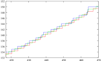
Figure 3: The bootstrapping of the spectral staircase (shown in red) by the $N^{(1)}(k)$ staircase (shown in green), bootstrapped in turn by the $N^{(2)}(k)$ staircase (shown in blue). Small vertical shift of $N^{(1)}(k)$ and $N^{(2)}(k)$ is given for illustration purposes. Note that the $N^{(2)}(k)$ does not bootstrap the $N^{(0)}(k)$. Data obtained for the “fully connected quadrangle” graph QGT .

These three properties of the auxiliary sequences $k^{(j)}_{n}$ allow to obtain the whole hierarchy explicitly. Starting from the periodic separators, one can find the roots $\hat{k}_{n}^{(r)}$ of the $r$th derivative of spectral determinant, then use them as separators on the next level of the hierarchy to find $\hat{k}_{n}^{(r-1)}$, and so on. After $r+1$ steps,

$$\hat{k}_{n}^{(j-1)}=\int_{\hat{k}_{n-1}^{(j)}}^{\hat{k}_{n}^{(j)}}\rho^{(j-1)}(k)\,kdk,$$ (10)

$j=r+1,...,1$, the spectrum $k_{n}$ is produced Fabula . The integrations (10) are made explicit by using the series expansions for the density $\rho^{(j)}(k)$ of the separators on each level of the hierarchy,

$$\rho^{(j)}(k)=\frac{L_{0}}{\pi}+\mathop{\rm Re}\sum_{p}S^{(j)}_{p}A_{p}^{(j)}e^{iS^{(j)}_{p}k}.$$ (11)

The weight coefficients $A_{p}^{(j)}$ and expansion frequencies $S^{(j)}$ in the expansions (11) are different for the different levels $j$ of the hierarchy For $j=0$ the series (11) is just the usual Gutzwiller’s formula.

Using (9) and (11) in (10) one can define each element in the $j$th separating sequence in terms of the elements of the previous one. The result is a set of equations that completely describe the propagation of the fluctuations across the hierarchy,

$$\delta_{n}^{(j-1)}=f^{(j-1)}_{\delta}-\sum_{p}C_{p}^{(j-1)}\sin\left(\omega_{p}^{(j-1)}n+\varphi^{(j-1)}_{p}\right),$$ (12)

where now the “zero frequency” term, $f^{(j-1)}_{\delta}=\left(\delta_{n}^{(j)}-\delta_{n-1}^{(j)}-(\delta_{n}^{(j)})^{2}+(\delta_{n-1}^{(j)})^{2}\right)/2$, the expansion coefficients, $C_{p}^{(j-1)}=\frac{2}{\pi}\frac{A_{p}^{(j-1)}}{\omega_{p}^{(j-1)}}\sin\frac{\omega_{p}^{(j-1)}}{2}\left(\delta_{n}^{(j)}-\delta_{n-1}^{(j)}+1\right)$, and the phases,

$$\varphi_{p}^{(j-1)}=\omega_{p}^{(j-1)}\left(\delta_{n}^{(j)}+\delta_{n-1}^{(j)}-1\right)/2$$ (13)

are functions of the fluctuations $\delta_{n}^{(j)}$ and $\delta_{n-1}^{(j)}$ on the previous level of the hierarchy. In the particular case when $r=0$, $\delta_{n}^{(1)}=1/2$, $n=1$, …, (12) coincides with the oscillating part of (1).

The properties of the fluctuation sequences outlined in this Section are inherited by other spectral characteristics, such as the nearest neighbor separations (Fig. 4), etc. The corresponding systems of equations that describe the propagation of these characteristics across the hierarchy are similar to (12) and can be easily derived from relating a particular spectral sequence to the one that precedes it in the hierarchy via (10).

IV Fluctuation Statistics

The expansions (12) allow to produce the probability distributions for the spectral fluctuations across the hierarchy, using the same approach as in Section II. By construction, the index $n$ is the same across the hierarchy, so the combinations (2) in the arguments of each of the trigonometric expansion terms in (12) produce uniformly distributed random variables $x_{i}$. This yields a discretized Itô type equation

$$\delta^{(j-1)}=f^{(j-1)}_{\delta}-\sum_{p}C_{p}^{(j-1)}\sin\left(\vec{m}^{(j-1)}_{p}\vec{x}+\varphi^{(j-1)}_{p}\right),$$ (14)

where $\delta_{1}^{(j)}$ and $\delta_{2}^{(j)}$ are also functions of $x$, produced by the corresponding expansions for $\delta_{n}^{(j)}$ and $\delta_{n-1}^{(j)}$. For a given $j$, these functions introduce the fluctuations from the lower levels of the hierarchy into (14).

It is possible to use the systems of expansions (12) directly to produce the probability distributions for each of the $\delta^{(j)}$s. However, it is more illustrative to use instead a simple physical approximation, in which the $j$th level fluctuations $\delta_{n}^{(j)}$ and $\delta_{n-1}^{(j)}$ are treated as independent random variables $\delta_{1}^{(j)}$ and $\delta_{2}^{(j)}$, distributed according to $P_{\delta}^{(j)}$. This allows to follow the accumulation of the fluctuations of the final distributions for $\delta^{(0)}$ starting from the fluctuations at the regular level, $\delta^{(r)}$.

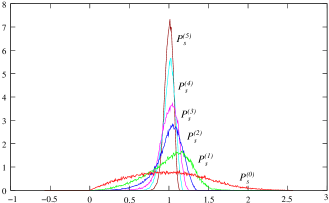
Figure 4: The development of the full scale spectral fluctuations for the nearest neighbor separations ($s^{(0)}$, shown in red) for the fully connected quadrangle graph studied also in QGT for $r=6$. One can follow the appearance of the Wignerian type distribution at the physical level from the distributions $P^{(j)}(s)$.

At the regular level, $j=r$, the fluctuations $\delta^{(r)}$ are described by an expansion structurally identical to (3) so the corresponding distribution $P_{\delta}^{(r)}$ is self-contained and has the same functional form as (5). Knowing $P_{\delta}^{(r)}$ allows to obtain $P_{\delta}^{(r-1)}$, and so on, up to the distribution $P_{\delta}^{(0)}$, which applies to the fluctuations of the physical momentum eigenvalues. With the independent $\delta_{1}^{(j)}$ and $\delta_{2}^{(j)}$ the transition from $P_{\delta}^{(j)}$ to $P_{\delta}^{(j-1)}$ is direct. Proceeding as in (3) -(6) yields the result

$$P_{\delta}^{(j-1)}(\delta^{(j-1)})=\int dke^{ik\delta^{(j-1)}}\left\langle F^{(j-1)}_{\delta}(k)\right\rangle_{\Omega^{(j-1)}},$$ (15)

where $F^{(j-1)}_{\delta}(k,\delta^{(j)})$ is obtained as (6) for the series (14), and $\langle*\rangle_{\Omega^{(j)}}$ represents averaging over the “disorder” produced by the separators $\delta_{1}^{(j)}$ and $\delta_{2}^{(j)}$ of $j$th level using the weight function

$$\Omega^{(j-1)}=e^{ikf^{(j-1)}_{\delta}\left(\delta_{1}^{(j)},\delta_{2}^{(j)}\right)}P_{\delta}^{(j)}\left(\delta^{(j)}_{1}\right)P_{\delta}^{(j)}\left(\delta^{(j)}_{2}\right)$$ (16)

Similar considerations produce the distributions for the nearest neighbor separations, the form factor, etc.

V Discussion

The explicit periodic orbit representations of the individual momentum eigenvalues $k_{n}$ of quantum graphs Fabula provide a regular analytical method of describing the statistical properties of their spectra within the standard periodic orbit theory framework.

As shown in Fabula , solving the spectral problem for a generic quantum graph goes beyond the conventional Gutzwiller’s theory approach. The additional information supplied by the auxiliary separating sequences $\hat{k}_{n}^{(j)}$ allows to produce the exact physical spectrum $k_{n}=\hat{k}_{n}^{(0)}$, to reveal the hierarchical structure of the spectral fluctuations and then to unfold the exact probability distributions for spectral statistics associated with each sequence $\hat{k}_{n}^{(j)}$.

Among other things, the expansions (3) also provide a physical understanding about the origins of the universal behavior of spectral characteristics based on the periodic orbit theory. It is known that the terms of lacunary trigonometric series behave as weakly dependent random variables (see e.g. Proxorov ; Revesz and the references therein). This fact allows to establish a number of universal features for the asymptotic distributions of their sums, such as convergence to Gaussian distribution with a specific variance (also conjectured to be the universal probability distribution profile for the $\delta^{(0)}_{n}$ distribution of generic quantum chaotic systems ABS ). In addition, the build up of the distributions $P^{(j)}$ along the levels of the hierarchy can lead to the appearance of other universal, (albeit more complex, e.g. Wignerian, see Fig. 4 and BGS ) profiles.

The advantage of this result is twofold. On the one hand, since the spectral properties of sufficiently complex quantum graphs are well described by the RMT QGT , the proposed approach provides a mechanism to follow the build up of the universal distributions as they appear at the top level of the spectral hierarchy. On the other hand, the analysis of a given system can be made as detailed as necessary (by using higher order approximations in each of the expansions (12)), (14), so the individual features are not overlooked behind broad universality.

Work supported in part by the Sloan and Swartz Foundations.

References

- (1) O. Bohigas, M.-J. Giannoni, C. Schmidt, Phys. Rev. Lett. 52, 1 (1984).
- (2) E. B. Bogomolny and J. P. Keating, Phys. Rev. Lett., Vol. 77, n 8, 1472 (1996). M. V. Berry, J. P. Keating and S. D. Prado, J. Phys. A: Math. Gen. 31 (1998) L245–L254.
- (3) T. Kottos and U. Smilansky, Phys. Rev. Lett. 79, 4794 (1997); Ann. Phys. 274, 76 (1999).
- (4) F. Barra and P. Gaspard, Phys. Rev. E 63, 066215 (2001); J. Stat. Phys. 101 pp. 283, (2000).
- (5) Y. Dabaghian and R. Blümel Phys. Rev. E 68, 055201(R) (2003); JETP Letters 77, n 9, p 530 (2003); Phys. Rev. E 70, 046206 (2004).
- (6) Y. Dabaghian, R. V. Jensen and R. Blümel JETP Letters 74, 258-262 (2001), JETP 121, N6 (2002).
- (7) R. Blümel Y. Dabaghian, R. V. Jensen, Phys. Rev. Lett. 88, 044101 (2002), Phys. Rev. E 65, 046222 (2002).
- (8) B. Ya. Levin, Distribution of Zeroes of Entire Functions, Am. Math. Society, Providence, (1980).
- (9) A. A. Karatsuba, Basic analytic number theory, Springer Verlag, (1993).
- (10) P. Revesz, (Ed.) Limit theorems in Probability and Statistics, Colloquia Mathematica S. 11, Keszthely, Hungary, (1974).
- (11) Yu.V.Prokhorov, V.A.Statulevicius (Eds.). Limit Theorems of Probability Theory, Springer, Berlin, (2000).
- (12) R. Aurich, J. Bolte, and F. Steiner, Phys. Rev. Lett. 73, 1356–1359 (1994).