Finite Controllability of Infinite-Dimensional Quantum Systems

Abstract

Quantum phenomena of interest in connection with applications to computation and communication almost always involve generating specific transfers between eigenstates, and their linear superpositions. For some quantum systems, such as spin systems, the quantum evolution equation (the Schrödinger equation) is finite-dimensional and old results on controllability of systems defined on on Lie groups and quotient spaces provide most of what is needed insofar as controllability of non-dissipative systems is concerned. However, in an infinite-dimensional setting, controlling the evolution of quantum systems often presents difficulties, both conceptual and technical. In this paper we present a systematic approach to a class of such problems for which it is possible to avoid some of the technical issues. In particular, we analyze controllability for infinite-dimensional bilinear systems under assumptions that make controllability possible using trajectories lying in a nested family of pre-defined subspaces. This result, which we call the Finite Controllability Theorem, provides a set of sufficient conditions for controllability in an infinite-dimensional setting. We consider specific physical systems that are of interest for quantum computing, and provide insights into the types of quantum operations (gates) that may be developed.

I Introduction

Over the last three decades, there has been a steady stream of papers in the physics/chemistry literature  HuangJMP1983 ; ShapiroJCP1986 ; TannorRice1 ; TannorRice2 ; PiercePRA88 that describe new experiments in atomic and molecular science, and new ways of thinking in which control-theoretic ideas are of central importance. More recently, the driving force has been the desire to manipulate quantum states in ways that would make possible quantum computation or quantum communication, see for example RanganPRA2001 ; KosloffPRL02 ; WhaleyPRA02 ; KhanejaPRA00 ; IvanovPRL03 ; JacobsPRL2007 . Phenomena involving the interaction between electromagnetic radiation (light) and matter (e.g. ions, spin states, etc.) are especially interesting because they are possible paradigms of future quantum computing devices QIC2001 . Many of the exciting ideas are related to the control of these systems (see for example, work on control of trapped-ion quantum states LawEberly ; KneerLaw ; BenKish ; BRBCDC2003 ; RanganPRL2004 ; RanganJMP2005 ). Some infinite-dimensional systems can be made to be effectively finite-dimensional by either bandwidth limits imposed by the control fields RanganPRA2001 , or by turning off specific transitions in order to truncate the Hilbert space RanganPRL2004 , and the controllability of such systems can be analyzed using finite-dimensional methods Brockett1972 ; Brockett1973 ; RamakrishnaPRA1995 ; Albertini .

We are interested in the quantum systems that are modelled as finite-dimensional for quantum computing purposes, when in fact they are infinite-dimensional. The well-known paper by Huang, Tarn and Clark HuangJMP1983 seems to be overly pessimistic with repect to the control of infinite quantum systems by asserting that “using piecewise-constant controls, global controllability cannot be achieved with a finite number of operations”. In 2000, Zuazua summarized the field aptly thus: ”From a mathematical point of view this [when the finite-dimensional system approaches the infinite-dimensional Schrödinger equation] is a very challenging (and very likely difficult) open problem in this area” Z2000 . Recently, Turinici and Rabitz TuriniciJPA2003 adapted the classical Ball-Marsden-Slemrod results BMS1982 to the quantum setting and showed that exact controllability does not hold in infinite-dimensional quantum systems (see also Beauchard2005 ). Along with an excellent review, Illner, Lange and Teismann TeismannESAIM2006 show that the Hartree equation that is well-known in quantum chemistry with bilinear control is not controllable in finite or infinite time. In spite of these negative results, most quantum computing systems that are indeed infinite-dimensional have shown themselves to be remarkably amenable to the production of a variety of states. Is it possible then to make a statement regarding the reachable set of states in such systems?

There has been recent progress in attacking this problem, and a few positive results. Ref. TuriniciCDC2000 showed that for an infinite-dimensional quantum control system with bounded control operators a quantum state could be steered only within a dense subspace of the relevant Hilbert space. In 2003 BRBCDC2003 , we showed that one can reach any finite linear superposition of states in a two-level system coupled to a harmonic oscillator by the alternate application of control fields even when one of the control operators is unbounded. Ref. ShapiroJCP2004 presents an ingenious method of creating arbitrary finite superpositions of rotational states of molecules by ensuring the trajectories lie within SU(N)[z,z-1] loop group of N-periodic matrices. Ref. KarwowskiPLA2004 presents a scheme that is well-known in atomic physics - when an infinite-dimensional quantum system has unequally spaced bound state energy levels, single resonant fields can be used to transfer population (albeit very slowly). Ref. LanJMP2005 provides a prescription for determining whether there exists a submanifold that is strongly analytic controllable, but this prescription does not identify the submanifolds. Ref. Adami2005 presents an adiabatic method of controlling a sequentially connected system in which the transition couplings get weaker as one moves away from the ground state. Ref. WuPRA2006 presents an algebraic framework to determine the nature of controllability of some infinite-dimensional quantum systems, specifically those with continuous spectra. Ref. Boscain2009 proves approximate controllability for bound states of quantum systems that are not equally spaced in energy even when the control matrices are unbounded.

We begin this paper in Section II by discussing the difficulties associated with applying traditional methods of analysis to infinite-dimensional control systems. We also discuss a specific class of infinite-dimensional systems — one in which it is desirable to steer a finite superposition of eigenstates to another finite superposition of eigenstates. We present a general theorem on Finite Controllability of quantum systems that exhibits the conditions needed for such transfers. For the specific quantum-computing models of interest, the trajectories are constrained to lie within subspaces. Section III presents examples of quantum-computing systems such as a model of a trapped-ion qubit and trapped-electron qubits. We show how our theorem can used to be prove finite controllability in the former case. We also discuss other similar systems where the theorem can and cannot be applied.

II Infinite-Dimensional Controllability

Controllability results for infinite-dimensional systems are seldom just straightforward extensions of the finite-dimensional ones, and in particular this is true for bilinear systems. Recently, there has been significant interest in the class of bilinear systems because of their relevance to quantum control. In the following subsection we illustrate the limitations of applying the tools of finite-dimensional systems analysis to certain classes of infinite-dimensional systems.

II.1 Limitations of Lie Algebraic analysis

Examining the Lie algebraic structure often gives us insights into the controllability of a quantum system, but in the case of infinite-dimensional systems, this insight is limited. In the well-known example of a resonantly-driven quantum harmonic oscillator (see e.g.  Schiffbook , BRBCDC2003 and Rouchon , the evolution is given by

$$\frac{\partial\psi}{\partial t}=\left(\omega\frac{i}{2}\left(\frac{\partial^{2}}{\partial x^{2}}-x^{2}\right)-iu(t)x\right)\psi.$$ (1)

Here, the bilinear control term $u(t)x$ arises because of the dipole interaction between the field and harmonic oscillator. The two operators of interest, $A=\frac{i}{2}\left(\frac{\partial^{2}\psi}{\partial x^{2}}-x^{2}\right)$ and $B=-ix$ generate a Lie algebra of skew-hermitian operators that is just four-dimensional. Thus, we expect that the control of this system will be limited. For example, it is well-known that it is not possible to transfer the number state $x(0)=|0\rangle$ to $x(T)=|n\rangle$ for $n>0$ ShoreBook using this control. We return to this example in Section III.

However, even when we encounter infinite-dimensional systems for which the Lie algebra also is infinite-dimensional (such as in Ref.LloydPRL1999 ; BRBCDC2003 ), the statements one can make about the controllability are also limited. More work is required to say with precision exactly what the reachable states are. This issue is illustrated in Section III.

In computing the span of the Lie algebra, it is necessary, of course that the domain of the operators involved be such that the bracket operations are allowable. This is the case in this paper, but we do not discuss these technical details here.

II.2 Finite Controllability

In this section, we prove an elementary but useful theorem about controllability on finite-dimensional subspaces of a complex Hilbert space. It is the basis for the applications we will present in the next section.

Definition 1

We will say that a finite-dimensional system evolving in the space of complex $n$-vectors $x$,

$$\dot{x}=\sum_{i}u_{i}G_{i}x$$

with skew-Hermitian operators $G_{i}$, is unit vector controllable if any unit length vector $x_{0}$ can be steered to any second unit length vector $x_{f}$ in finite time.

Theorem 2 (Finitely Controllable Infinite Dimensional Systems)

Consider a complex Hilbert space $\mathcal{X}$ together with a nested set of finite-dimensional subpaces $\mathcal{H}=\{\mathcal{H}_{1}\subset\mathcal{H}_{2}\subset\mathcal{H}_{3}...\}$. Consider

$$\dot{x}=(\sum_{i=1}^{m}u_{i}G_{i})x.$$

Assume that $\mathcal{H}_{1}$ is an invariant subspace for a subset $\mathcal{G}_{1}$ of the set $\{G_{i}\}$ and that the system is unit vector controllable on $\mathcal{H}_{1}$ using only this subset of the $G_{i}$. If for each $\mathcal{H}_{\alpha}\;\alpha\neq 1$ there is a subset $\mathcal{G}_{\alpha}$ of $\{G_{i}\}$ that leaves $\mathcal{H}_{\alpha}$ invariant and if for any unit vector in $\mathcal{H}_{\alpha}$ the orbit generated by exp $\left(\mathcal{G}_{\alpha}\right)$ contains a point in one of the lower dimensional subspaces $\mathcal{H}_{\beta}$ then any unit vector in any of the $\mathcal{H}_{i}$ can be steered to any other unit vector in any other $\mathcal{H}_{j}$ using a finite number of piecewise constant controls.

Remark: Given a system and a nested set of finite dimensional subspaces it will be said to be finitely controllable if it can be transfered from any point in one of the subpaces to any other point in that subspace with a trajectory lying entirely within the subspace.

Proof: Suppose that $x(0)\in\mathcal{H}_{\alpha}$ and $x(T)\in\mathcal{H}_{\beta}$ are unit vectors representing the initial value of $x$ and the desired final value, respectively. Then by assumption either there exists a subset of the $\{G_{i}\}$ that leaves $\mathcal{H}_{\alpha}$ invariant and steers $x(0)$ to a point in some $\mathcal{H}_{\beta}$ with the dimension of $\mathcal{H}_{\beta}$ being strictly less than that of $\mathcal{H}_{\alpha}$ or else $x(0)\in\mathcal{H}_{1}$. A finite induction on the index of the set $\mathcal{H}_{i}$ then shows that the state can be steered to a unit vector in the subspace $\mathcal{H}_{1}$, which is a controllable subspace. To finish the proof, observe that if one can reach $x_{a}\in\mathcal{H}$ from $x_{b}\in\mathcal{H}$ then the standard time reversal argument using the fact that the $G_{i}$ are skew-Hermetian shows that it is possible to reach $x_{b}\in\mathcal{H}$ from $x_{a}\in\mathcal{H}$. Thus a second application of the steps given above implies that it is possible to reach $x(T)\in\mathcal{H}_{\beta}$.

Discussion and example: Various technical issues that arise in infinite-dimensions illustrate the significance of this theorem. All finite-dimensional subspaces are closed in the usual topology but infinite-dimensional subspaces need not be and there are a number of issues involving infinite-dimensional controllability that can be clarified by giving more attention to the distinction. Let $l_{2}$ denote the Hilbert space of infinite vectors whose entries are square summable which corresponds to the entire state space of our quantum system. Let $l_{0}$ denote the subspace consisting of those elements with only a finite number of nonzero entries, which corresponds in our setting to a finite superposition of states. Of course, this subspace is not closed.

We recall now some general ideas from operator theory Dunford and discuss their relationship to our theorem.

1. If $e^{A}$ and $e^{B}$ are bounded operators mapping a Hilbert space $\mathcal{H}$ into itself and if $\mathcal{V}$ is an invariant subspace for $e^{A}$ and $e^{B}$, then $\mathcal{V}$ is invariant for the product $e^{A}e^{B}$.

   In our setting $e^{B_{c}}$ and $e^{B_{r}}$ are unitary and thus bounded.

2. If $A$ is the infinitesimal generator of a semigroup mapping a Hilbert space $\mathcal{H}$ into itself and if $\mathcal{V}$ is a closed, nontrivial, invariant subspace for $A$, then $\mathcal{V}$ is invariant subspace for $e^{At}$.

   Consider for example an operator $A$ on $l_{2}$ that maps the $i^{th}$ unit basis vector $e_{i}$ into $e_{i+1}$ for all $i=1,2,...$. This operator clearly sends $l_{0}$ into itself but $e^{At}$ for $t\neq 0$ sends $e_{1}$ into the element $\sum_{i}e_{i}t^{i}/i!$ which is not in $l_{0}$.

3. If $A$ and $B$ are infinitesimal generators of a semigroup mapping a Hilbert space $\mathcal{H}$ into itself and if $\mathcal{V}$ is a closed, invariant subspace for $A$ and $B$, then $\mathcal{V}$ is invariant subspace for $e^{(A+B)t}$.

   Again, the assumption that $\mathcal{V}$ is closed cannot be dispensed with. For example, consider a system $\dot{x}=uAx+vBx$ with $A$ being block diagonal with two-by-two blocks and $B$ being basically block diagonal with two-by-two blocks except for top and left borders where the necessary one-by-one, two-by one and one-by two matrices pad an otherwise block diagonal matrix. Specifically, $A$ and $B$ are given by

   $$A =\left[\begin{array}[]{ccccc}B_{0}&0_{22}&0_{22}&0_{22}&...\\ 0_{22}&B_{0}&0_{22}&0_{22}&...\\ 0_{22}&0_{22}&B_{0}&0_{22}&...\\ 0_{22}&0_{22}&0_{22}&B_{0}&...\\ ...&...&...&...&...\end{array}\right]\;\;;\;\;$$ (7)

   $$B =\left[\begin{array}[]{ccccc}0_{11}&0_{12}&0_{12}&0_{12}&...\\ 0_{21}&B_{0}&0_{22}&0_{22}&...\\ 0_{21}&0_{22}&B_{0}&0_{22}&...\\ 0_{21}&0_{22}&0_{22}&B_{0}&...\\ ...&...&...&...&...\end{array}\right],$$ (13)

   with $0_{ij}$ denoting an $i$ by $j$ matrix of zeros and

   $$B_{0}=\left[\begin{array}[]{cc}0&1\\ -1&0\end{array}\right].$$ (16)

   The operators $A$ and $B$ leave $l_{0}$ invariant but the exponential of their sum does not.

One can provide a direct argument not involving Lie theoretic techniques that shows that any unit vector can be transferred to $e_{1}$. The idea, motivated by the analysis in Ref. LawEberly , is to alternate the use of $A$ and $B$ and reason that if we start with a vector with $x_{n}\neq 0$ and $x_{m>n}=0$ we can use a control with $v=0$ (or $u=0$ depending on whether $n$ is even or odd) to reduce the vector to one for which $x_{n}$ is zero, then use a control with $u=0$ to reduce the vector to one with $x_{n-1}=0$ without changing $x_{n}$, etc. This argument depends on observing that

$$e^{Au}= \left[\begin{array}[]{ccccc}e^{B_{0}u}&0_{22}&0_{22}&0_{22}&...\\ 0_{22}&e^{B_{0}u}&0_{22}&0_{22}&...\\ 0_{22}&0_{22}&e^{B_{0}u}&0_{22}&...\\ 0_{22}&0_{22}&0_{22}&e^{B_{0}u}&...\\ ...&...&...&...&...\end{array}\right]\;\;;\;\;$$ (22)

$$e^{Bv}= \left[\begin{array}[]{ccccc}1&0_{12}&0_{12}&0_{12}&...\\ 0_{21}&e^{B_{0}v}&0_{22}&0_{22}&...\\ 0_{21}&0_{22}&e^{B_{0}v}&0_{22}&...\\ 0_{21}&0_{22}&0_{22}&e^{B_{0}v}&...\\ ...&...&...&...&...\end{array}\right]$$ (28)

from which we see that $e^{Au}$ simply rotates the entries in $x$ pairwise, i.e., $x_{1},x_{2}$; $x_{3},x_{4}$; etc. so that by attending only to the subspace defined by $x_{n}$ and $x_{n-1}$ one can make $x_{n}=0$. Having done so, we can use $e^{Bv}$ to rotate in $x_{n-1},x_{n-2}$ space so as to reduce $x_{n-1}=0$ with out changing $x_{m>n-1}$, etc. This shows that the Lie group generated by $e^{Au}$ and $e^{Bv}$ acts transitively on the unit vectors and thus identifies the Lie algebra to within one of a few possibilities. (See Ref. Brockett1973 ).

III Physical Systems

In this section, we apply the Finite Controllability Theorem to determine the reachable set of states of four infinite-dimensional quantum systems, namely, the quantum harmonic oscillator, a spin-half system coupled to a harmonic oscillator (model of a trapped-ion qubit), an N-level atom coupled to harmonic oscillator, and a spin-half system coupled to two harmonic oscillators (model of a trapped electron qubit). Note that in all sections below we use atomic/scaled/dimensionless units so that the evolution equations do not explicitly contain Planck’s constant $\hbar$, the charge of the electron $e$ or the mass of the electron $m_{e}$.

III.1 System 1: Quantum harmonic oscillator

We discuss this well-known system first. The controllability algebra is finite-dimensional and, in particular, the system does not satisfy the conditions needed for the application of the Finite Rank Controllability Theorem. The discussion, however, is key to setting up the formalism used in subsequent examples that are finitely controllable.

The problem of controlling the harmonic oscillator has been discussed many times (see e.g. HOcontrol and other references as discussed above). If the control is a sinusoidal resonant driving field (of frequency equal to the harmonic oscillator frequency $\omega_{m}$) as shown in the transfer graph Fig. 1, then the evolution is via

$$\frac{\partial\psi}{\partial t}=\left(\omega_{m}\frac{i}{2}\left(\frac{\partial^{2}}{\partial x^{2}}-x^{2}\right)-iu(t)x\right)\psi.$$ (29)

Here, the control term $u(t)x$ arises because of the dipole interaction between the field and harmonic oscillator. The operators of interest are $A=\frac{i}{2}\left(\frac{\partial^{2}}{\partial x^{2}}-x^{2}\right)$ and $B=-ix$. $A$ and $B$ generate a Lie algebra of skew-hermitian operators that is just four-dimensional ($C=[A,B]=\frac{\partial}{\partial x}$, $D=[B,C]=iI$, where $I$ is the identity operator). This in itself tells us that the resonantly driven harmonic oscillator is not controllable.

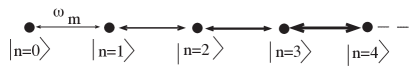
Figure 1: Graphical representation of the quantum harmonic oscillator driven by a sinusoidal resonant field. Note that while the strengths of the transition couplings increase as the square root of the quantum number $n$ as shown by the boldness of the connections between energy levels, the transition frequency between each level is the same. It is this latter property that leads to a lack of controllability.

As is well-known, the spectrum of $A$ is discrete. If we describe the evolution in terms of an eigenfunction expansion, with the basis being $|n\rangle$’s, the eigenfunctions of $\partial^{2}/\partial x^{2}-x^{2}$, then the evolution is via

$$\dot{x}_{n} = -i\omega_{m}(n+\frac{1}{2})x_{n}$$

$$-u(t)\frac{i}{\sqrt{2}}(\sqrt{n-1}x_{n-1}-\sqrt{n}x_{n+1}).$$

Although the eigenstates of the harmonic oscillator can be written as an infinite set of nested finite subspaces, it is seen that the operator $B$ connects space $\mathcal{H}_{i}$ to both $\mathcal{H}_{i-1}$ and $\mathcal{H}_{i+1}$. Thus finite superpositions of eigenstates may not be reached by resonantly driving the harmonic oscillator, consistent with the fact that the requirements of the Finite Controllability Theorem are not met. Physically, this is due to the degeneracy of spacings between the eigenstates and the fact that the control vector field simultaneously illuminates all states.

However, the system is in fact partially controllable. One can be quite explicit about the reachable wave functions under the application of a control ShoreBook . It is interesting that the finite-dimensionality of the algebra that makes the system uncontrollable is also the property that makes it possible to derive an analytic expression for the unitary propagator Rau . For example, if we agree to call any function of $t$ and $x$ which has the form

$$\psi(0,x)=k(t)e^{i(a(t)x^{2}+b(t)x)}$$ (31)

i-gaussian , then if the initial value of $\psi$ is i-gaussian the solution will be i-gaussian for all time, regardless of the choice of $u(t)$. (This is directly analogous to the fact that the solution of the conditional density equation of estimation theory remains gaussian if it has a gaussian initial condition.) An example of such a function is the well-known coherent state GlauberPRL1963

$$|\alpha\rangle=\exp(-|\alpha|^{2}/2)\sum_{n=0}^{\infty}\frac{\alpha^{n}}{n!}|n\rangle.$$ (32)

We see that it is not possible to transfer $x(0)=|\alpha\rangle$ to $x(T)=|i\rangle$ for $i>0$ because $|i\neq 0\rangle$ is not i-gaussian, but $|\alpha\rangle$ is, and is in fact a coherent state.

III.2 System 2: Spin-half particle in a quadratic potential

In contrast to the harmonic oscillator, the model of a spin-half particle coupled to a harmonic oscillator with suitable controls turns out to be finitely controllable. This model is a good representation of an ion with two essential internal states trapped in a quadratic potential. We show below that this system satisfies the conditions of the Finite Controllability Theorem of Section 2. Moreover, one can also provide an algorithm for explicit control. The spin-$\frac{1}{2}$ model represents a two-level atomic ion with an energy splitting $\hbar\omega_{0}$, where the frequency $\omega_{0}/2\pi$ is in the several GHz range. The atomic levels are coupled to the motion of the ion in a harmonic trap WinelandNISTreport1998 . These quantized vibrational energy levels are separated by a frequency $\omega_{m}/2\pi$ in the MHz range.

In a frequently cited paper, Law and Eberly LawEberly showed that when properly interpreted, this system has interesting controllability properties, quite different from the properties of the harmonic oscillator alone. In fact, by coupling the harmonic oscillator with a two-level system it is possible to arrive at a system which is much more controllable than the harmonic oscillator. At an intuitive level, this can be seen simply as a consequence of the fact that the addition of a spin degree of freedom breaks the infinite degeneracy associated with the harmonic oscillator and allows the system to resonate with more than one frequency. This allows the transfer of population from any eigenstate to any other eigenstate by sequentially applying the two frequencies. We now analyze this system from a controllability viewpoint.

An eigenstate of the spin-half system coupled to a quantum harmonic oscillator is denoted by $|S,n\rangle$, where the first index refers to the “spin” state of the system, and the second index is the number state of the harmonic oscillator. An applied field causes transitions between the eigenstates of the coupled spin-oscillator system. A monochromatic field of angular frequency $\omega=\omega_{0}$ causes resonant transitions between states $|\downarrow,n\rangle$ and $|\uparrow,n\rangle$ (carrier or spin-flip transitions). A monochromatic field of angular frequency $\omega=\omega_{0}-\omega_{m}$ causes resonant transitions between states $|\downarrow,n\rangle$ and $|\uparrow,n-1\rangle$, i.e., produces so called red sideband (that is with angular frequency $\omega=\omega_{0}-\omega_{m}$) transitions.

These transitions are graphically depicted in Fig. 2 with the thickness of the edges qualitatively representing the strength of the coupling between the states. As pointed out in Ref. RanganJMP2005 , when both fields (carrier and red sideband) are applied simultaneously, the eigenstates of the system are sequentially connected. Therefore, we look at the trapped-ion model controlled only by these two fields.

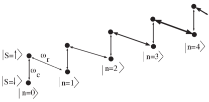
Figure 2: Graphical representation of the coupled spin-half quantum harmonic oscillator system driven by sinusoidal resonant fields of angular frequency $\omega_{c}$ and $\omega_{r}$ as shown. When $\eta\ll 1$, the strengths of the $\omega_{c}$ transition couplings are independent of the harmonic oscillator quantum number $n$, whereas the strengths of the $\omega_{r}$ transition couplings increase as the square root of $n$ as shown by the boldness of the coupling lines. Note that there is no direct coupling between two consecutive oscillator states with fixed spin.

Now we write the evolution equation of the spin-half coupled to harmonic oscillator driven by two fields that drive the carrier and red sideband transitions. The amplitudes corresponding to the fields that cause the carrier and red transitions are dubbed $E_{c}$ and $E_{r}$ respectively. As detailed in Appendix References, in the interaction picture and in the energy eigenbasis, the evolution equation is written as

$$\dot{Y} = (u(t)B_{c}+v(t)B_{r})Y.$$ (33)

The controls $u(t)$ and $v(t)$ are related to the applied fields via the equations

$$u(t) = c_{1}E_{c}(t)=0.25\mu\exp(-\eta^{2}/2)E_{c}(t),$$ (34)

$$v(t) = c_{2}E_{r}(t)=0.25\eta\mu\exp(-\eta^{2}/2)E_{r}(t).$$ (35)

Here $\eta$, the so-called Lamb-Dicke parameter, is the product of $k$, wave vector of the light, and $x_{0}$, the amplitude of the zero-point motion of the particle in the harmonic potential (or the spatial extent of the ground state harmonic oscillator wave function). By ordering the eigenstates as $|\uparrow,0\rangle,\ |\uparrow,1\rangle,\ \ldots,|\downarrow,0\rangle,\ |\downarrow,1\rangle,\ \ldots$, the control matrices are written as

$$B_{c} = \left(\begin{array}[]{c|c}0&iL_{0}\\ \hline\cr iL_{0}^{T}&0\\ \end{array}\right).$$ (38)

$$B_{r} = \left(\begin{array}[]{c|c}0&L_{1}\\ \hline\cr-L_{1}^{T}&0\\ \end{array}\right).$$ (41)

The upper-triangular matrices $L_{0}$ and $L_{1}$ are defined as

$$L_{0} = \left(\begin{array}[]{cccc}L_{0}(\eta^{2})&0&0&\ldots\\ 0&L_{1}(\eta^{2})&0&\ldots\\ 0&0&L_{2}(\eta^{2})&\ddots\\ \vdots&\vdots&\vdots&\ddots\\ \end{array}\right).$$ (46)

$$L_{1} = \left(\begin{array}[]{cccc}0&L_{0}^{(1)}(\eta^{2})&0&\ldots\\ 0&0&L_{1}^{(1)}(\eta^{2})&\ldots\\ 0&0&0&\ddots\\ \vdots&\vdots&\vdots&\ddots\\ \end{array}\right).$$ (51)

This structure of the control Hamiltonian precludes the use of adiabatic methods such as those used in Ref. Adami2005 . Unlike the situation encountered in the analysis of the quantum harmonic oscillator algebra, here the formal commutation of the operators $B_{c}$ and $B_{r}$ does not lead to a finite-dimensional algebra, suggesting that the model with spin is much more controllable. This is the case, as will be explored in the next subsection.

III.2.1 Controllability: Lie Algebra

It is interesting to compare our analysis with the formal calculations suggested by Lie theory. The first thing to do is to determine the formal structure of the Lie algebra, which we now consider.

The control of the trapped-ion system is often studied in two different limiting cases - one in which the extent of zero-point motion of the spin-half particle in the harmonic potential $x_{0}$ is much smaller than the wavelength of the applied light $2\pi/k$, i.e., $\eta\ll 1$ (the Lamb-Dicke limit), and the other in which $\eta\simeq 1$ (beyond the Lamb-Dicke limit). The case in which $\eta\simeq 1$ is more general than the case of the Lamb-Dicke limit, but requires a more sophisticated analysis. We study initially the Lamb-Dicke limit in which the Lamb-Dicke parameter $\eta\ll 1$. The terms in equations (46) and (51) are expanded to first order in $\eta$. The control Hamiltonians can then be expressed in operator form as

$$B_{c} =\left[\begin{array}[]{cc}0&i\\ i&0\end{array}\right],\ {\rm and}$$ (54)

$$B_{r} =\eta\left[\begin{array}[]{cc}0&a\\ -a^{{\dagger}}&0\end{array}\right],$$ (57)

where $a$ and $a^{{\dagger}}$ denote the annihilation and creation operators of the harmonic oscillator as defined in Appendix References. (Note that $B_{r}$ is the same Hamiltonian as obtained from the well-known Jaynes-Cummings model JaynesCummings that describes the interaction between a quantized cavity field and a two-level atom.)

In order to compute the Lie algebra, let us consider $T$, an operator acting on a complex Hilbert space. We associate with $T$ a skew-hermitian operator acting on $\mathcal{H}\oplus\mathcal{H}$ defined by

$$J(T)=\left[\begin{array}[]{cc}0&T\\ -T^{\dagger}&0\end{array}\right].$$ (60)

For convenience, let $K(T)$ be another operator defined in a similar way as

$$K(T)=\left[\begin{array}[]{cc}T&0\\ 0&-T\end{array}\right].$$ (63)

Of course, $K(T)$ is skew-hermitian if and only if $T$ is. The control operators we are interested in for the purposes of determining the structure of the Lie algebra are given by $B_{c}=J(iI)$ and $B_{r}=\eta J(a)$. We have

Lemma 3

The Lie algebra generated by $J(iI)$ and $J(T)$ includes the operators

$$J(W^{2p});\;p=1,2,3,\cdots\;;\;K(W^{2p+1});\;p=0,1,2,\cdots\ ,$$ (64)

where, $W=i(T+T^{\dagger})$.

Proof: A calculation shows that $[J(T),J(iI)]=K(W)$ and further, $[J(iI),K(W)]=-2iJ(W)$. We can then check that

$$ad_{J(W)}^{p}(K(W))=(-2)^{p}\left\{\begin{array}[]{ll}J(W^{p+1}),\;{\rm if\ p\ is\ odd}\\ K(W^{p+1}),\;{\rm if\ p\ is\ even}\end{array}\right\}.$$ (67)

These calculations make it clear that if the powers of $W$ are independent then $J(iI)$ and $J(T)$ do not generate a finite-dimensional algebra. Thus if T is nonzero only on the diagonal immediately above the main diagonal (which is true for the operator $a$), and if every term on this upper-diagonal is nonzero, then the successive powers of $W$ are independent and the algebra is infinite-dimensional.

This is the case for the coupled spin-half harmonic oscillator system. Of course, this calculation only shows that this system, unlike the harmonic oscillator, does not generate a finite-dimensional controllability Lie algebra. More work is required to say with precision exactly what the reachable states are. This is precisely the role of Theorem 2 which gives more specific information of which operators play a role in the control process.

Note: In the case where the Lamb-Dicke limit does not apply, the Lie algebra will still be infinite-dimensional but the terms are more complicated.

III.2.2 Finite controllability

In this subsection we discuss how finite controllability works in this infinite-dimensional setting.

From Fig. 2, it is seen that the sequentially connected eigenstates can be looked at as an infinite set of finite-dimensional subspaces with the ground state $|\downarrow,0\rangle$ being equal to $\mathcal{H}_{1}$. Further, when operators $B_{c}$ and $B_{r}$ are applied sequentially, each subspace $H_{i}$ can be transferred to $\mathcal{H}_{i-1}$. Thus the criteria for finite controllability are met. By sequential application of the two operators, any finite superposition of eigenstates can be transferred to the ground state in finite time.

The application of these statements to the spin-half in quadratic potential example is best understood by writing the control matrices $B_{c}$ and $B_{r}$ in a re-ordered basis as follows: The eigenstates can be ordered as $|\uparrow,0\rangle,\ |\uparrow,1\rangle,\ \ldots,|\downarrow,0\rangle,\ |\downarrow,1\rangle,\ \ldots$. In the interaction picture, the Schrödinger equation is written as

$$\dot{Y} = (u(t)B_{c}+v(t)B_{r})Y,$$ (68)

where $u(t)$ and $v(t)$ are defined as before. Then,

$$B_{c} = i\left(\begin{array}[]{cc|cc|cc|c}0&L_{0}&0&0&0&0&\ldots\\ L_{0}&0&0&0&0&0&\ldots\\ \hline\cr 0&0&0&L_{1}&0&0&\ldots\\ 0&0&L_{1}&0&0&0&\ldots\\ \hline\cr 0&0&0&0&0&L_{2}&\ldots\\ 0&0&0&0&L_{2}&0&\ldots\\ \hline\cr\vdots&\vdots&\vdots&\vdots&\vdots&\vdots&\ddots\\ \end{array}\right).$$ (76)

$$B_{r} = \left(\begin{array}[]{c|cc|cc|cc}0&0&0&0&0&0&\ldots\\ \hline\cr 0&0&L_{0}^{(1)}&0&0&0&\ldots\\ 0&-L_{0}^{(1)}&0&0&0&0&\ldots\\ \hline\cr 0&0&0&0&L_{1}^{(1)}&0&\ldots\\ 0&0&0&-L_{1}^{(1)}&0&0&\ldots\\ \hline\cr 0&0&0&0&0&0&\ldots\\ \vdots&\vdots&\vdots&\vdots&\vdots&\vdots&\ddots\\ \end{array}\right).$$ (84)

$L_{i}$’s and $L_{i}^{(1)}$’s are Laguerre polynomials of the zeroth and first order, all with argument $\eta^{2}$.

One can immediately see the applicability of the general statements made in the subsection 2 to this system. The model of the trapped-ion qubit highlights the existence of important examples for which it is desirable for the evolution to occur on a non-closed subspace of a Hilbert space, i. e., the space of finitely nonzero elements. In this model, this non-closed subspace consists of vectors in the oscillator representation with finitely many nonzero elements. The $B_{c}$ and $B_{r}$ operators and their one parameter groups, leave invariant the subspace $l_{0}$ of $l_{2}$ consisting of finitely nonzero sequences. The semigroup $e^{\alpha B_{c}+\beta B_{r}}$ will not, however, typically have any nontrivial invariant subspace. To satisfy the requirements of the Finite Controllability Theorem one never uses a linear combination of the operators. Further, as we have seen, the key to controllability is that each operator has a different invariant subspace within the set of finite superpositions.

III.2.3 Explicit finite controllability scheme

The property that both control vector fields are never used simultaneously is exploited by Law and Eberly LawEberly and Kneer and Law KneerLaw in order to devise a explicit scheme for the production of a finite superposition of eigenstates from another finite superposition in the control of a spin-half particle coupled to a harmonic oscillator (in the Lamb-Dicke limit). It shows that if $x$ can be transferred to $y$ by a series of such “single nonzero $u_{i}$” moves then the transfer from $y$ to $x$ is also possible.

Specifically the Law-Eberly scheme LawEberly to transfer any eigenstate $|i\rangle$ to any other eigenstate $|j\rangle$ involves the alternate use of transitions generated by spin reversal ($\pi$-pulses of $E_{c}$) and transitions generated by $\pi$-pulses of $E_{r}$ which convert from a state in which the oscillator has energy $E_{i}$ and spin down to a state in which the energy of the oscillator in altered by one unit and the spin is flipped as well (see equation (57)). For example suppose we wish to drive a state from the $|\downarrow,n\rangle$ to $|\uparrow,n-2\rangle$ (see Fig. 2). This can be done using $B_{r}$ to drive the system from $|\downarrow,n\rangle$ to $|\uparrow,n-1\rangle$, $B_{c}$ to drive the system from $|\uparrow,n-1\rangle$ to $|\downarrow,n-1\rangle$ and finally $B_{r}$ to go from $|\downarrow,n-1\rangle$ to $|\uparrow,n-2\rangle$.

We note that this scheme works both in the Lamb-Dicke limit and beyond the Lamb-Dicke limit. In the Law-Eberly scheme, the $\pi$-pulses of $E_{c}$ are all of the same time duration because in the Lamb-Dicke limit, all the carrier transitions are equally strong. However, the coupling strengths of the red-sideband transitions are proportional to $\sqrt{n}$, and therefore the $\pi$-pulses of $E_{r}$ are shorter in duration as eigenstates of higher $n$ are addressed. In order to generate an arbitrary superposition of a finite number of eigenstates, starting from another arbitrary superposition, an additional trick is to go through the ground state of the system which acts as a “pass state” TuriniciReview2000 . It is possible to provide an explicit algorithm which will drive the system from any finite superposition to any other finite superposition.

To prepare an arbitrary finite superposition, the simplest path is to take the system through the ground state. One assumes that the desired state is the initial state and then designs a sequence of alternating pulses of the $E_{c}$ and $E_{r}$ fields that would take this state to the ground state $|\downarrow,0\rangle$ KneerLaw . The actual sequence that produces the superposition is the time-reversed sequence that was designed. For example, if the desired superposition is $(|\uparrow,3\rangle+|\downarrow,2\rangle)/\sqrt{2}$, the sequence of pulses that will transfer this state to the ground state is $E_{c}^{(1)}(\pi)\$$E_{r}^{(2)}(\phi_{2})\ E_{c}^{(3)}(\phi_{3})\ E_{r}^{(4)}(\phi_{4})\ E_{c}^{(5)}(\phi_{5})\ E_{r}^{(6)}(\phi_{6})\ E_{c}^{(7)}(\phi_{7}).$ The action of each pulse is the following: $E_{c}^{(1)}$ is a $\pi$ pulse of the carrier field that moves the state $|\uparrow,3\rangle$ to $|\downarrow,3\rangle$. (Simultaneously, the population in $|\downarrow,2\rangle$ is transferred to $|\uparrow,2\rangle$). $E_{r}^{(2)}$ is a pulse of the red-sideband field that moves between the states $|\downarrow,3\rangle$ and $|\uparrow,2\rangle$. Since there is already a superposition of the two states, the duration of the red-sideband field is shorter than that of a $\pi$-pulse. Simultaneously, a superposition of $|\downarrow,2\rangle$ and $|\uparrow,1\rangle$ is created. The next transition $E_{c}^{(3)}(\phi_{3})$ transfers population between $|\uparrow,2\rangle$ and $|\downarrow,2\rangle$, and again is shorter than a $\pi$ pulse. This sequence progresses till all the population is in $|\downarrow,0\rangle$. The actual sequence is the time-reversed sequence of the one that is described above — this creates the desired superposition from the initial ground state.

If one were to transfer an arbitrary initial superposition to an arbitrary final superposition of eigenstates, one employs the above algorithm twice. The sequences A and B that take the system from the initial and final superpositions respectively to the ground state are first calculated. Then the sequence A is first applied taking all the population to the ground state. The time time-reversed sequence of B is then applied which takes the population to the desired final superposition. Clearly, this scheme works in finite time only if the initial and final states are both superpositions of a finite number of states.

Note that finite superpositions are dense in the Hilbert space of all possible states. Hence from our Lie algebra analysis and the use of the Law-Eberly algorithm we have

Proposition 4

The span of the Lie algebra generated by the operators $B_{c}$ and $B_{r}$ for the quantum control system in Eq. (33) is infinite-dimensional and the reachable set, which is dense in the Hilbert space of all states, includes all finite superpositions.

Note that this provides an explicit dense subspace controllability result which is hard to prove by abstract methods (see BMS1982 and Z2000 ). Note also that the proof of controllability that Law and Eberly give of what they term “arbitrary control” might be more accurately described as demonstrating that any state in $l_{0}$ can be mapped to any other state in $l_{0}$, staying within $l_{0}$ (see the discussion in subsection 2).

III.2.4 Red and blue sideband controlled trapped-ion qubit

The importance of the requirement of the Finite Controllability Theorem that the the system is unit vector controllable on $\mathcal{H}_{1}$ is seen by examining the trapped-ion qubit driven by the red and blue sideband fields alone. Recall that a monochromatic field of frequency $\omega=\omega_{0}-\omega_{m}$ ($\omega=\omega_{0}+\omega_{m}$) causes resonant transitions between states $|\downarrow,n\rangle$ and $|\uparrow,n-1\rangle$ ($|\downarrow,n\rangle$ and $|\uparrow,n+1\rangle$), i.e., produces red (blue) sideband transitions. The Schrödinger equation in the interaction picture is written as

$$\dot{Y} = (v_{1}(t)B_{r}+v_{2}(t)B_{b})Y,$$ (85)

where $v_{1}(t)$ and $v_{2}(t)$ are of the form of $v(t)$ defined before. Then in terms of the Laguerre polynomials of the first order and with argument $\eta^{2}$,

$$B_{r} = \left(\begin{array}[]{c|cc|cc|cc}0&0&0&0&0&0&\ldots\\ \hline\cr 0&0&L_{0}^{(1)}&0&0&0&\ldots\\ 0&-L_{0}^{(1)}&0&0&0&0&\ldots\\ \hline\cr 0&0&0&0&L_{1}^{(1)}&0&\ldots\\ 0&0&0&-L_{1}^{(1)}&0&0&\ldots\\ \hline\cr 0&0&0&0&0&0&\ldots\\ \vdots&\vdots&\vdots&\vdots&\vdots&\vdots&\ddots\\ \end{array}\right).$$ (93)

$$B_{b} = \left(\begin{array}[]{cc|cc|cc|c}0&0&0&L_{0}^{(1)}&0&0&\ldots\\ 0&0&0&0&0&0&\ldots\\ \hline\cr 0&0&0&0&0&L_{1}^{(1)}&\ldots\\ -L_{0}^{(1)}&0&&0&0&0&\ldots\\ \hline\cr 0&0&0&0&0&&\ldots\\ 0&0&-L_{1}^{(1)}&0&&0&\ldots\\ \hline\cr\vdots&\vdots&\vdots&\vdots&\vdots&\vdots&\ddots\\ \end{array}\right).$$ (101)

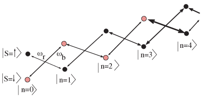
Figure 3: Graphical representation of the coupled spin-half quantum harmonic oscillator system driven by sinusoidal resonant fields $\omega_{r}$ and $\omega_{b}$ as shown. The strengths of the $\omega_{r}$ and $\omega_{b}$ transition couplings increase as the square root of $n$.

From Fig. 3, it is seen that the sequentially connected eigenstates can be looked at as an infinite set of finite-dimensional subspaces with the space consisting of $|\downarrow,0\rangle$ and $|\uparrow,0\rangle$ being equal to $\mathcal{H}_{1}$. Further, when operators $B_{r}$ and $B_{b}$ are applied sequentially, each subspace $\mathcal{H}_{i}$ can be transferred to $\mathcal{H}_{i-1}$. However, by sequential application of the two operators, any finite superposition of eigenstates cannot be transferred to the ground state in finite time. This is because the subspace $\mathcal{H}_{1}$ is not transitively connected and therefore not unit vector controllable.

Note that this is a special case because these two control fields split the Hilbert space into two unconnected subspaces (denoted in the graph by the states with the grey nodes and the black nodes). In each of these subspaces, the Finite Controllability Theorem holds. That is, one might transfer finite superpositions to other finite superpositions in one subspace or the other.

III.3 System 3: Control of an N-level ion trapped in a quadratic potential

We note that the above example may be extended to models of an $N$-level system coupled to a quantum harmonic oscillator. Without loss of generality, it can be assumed that the energy levels in the $N$-level system are not equally spaced (for example atomic levels). If $N-1$ monochromatic, resonant fields are available to couple every pair of adjacent energy levels, the $N$-level system itself is transitively connected. It is necessary to have one more control field in order to make the $\mathcal{H}_{i}$ to $\mathcal{H}_{i-1}$ transition (ladder transition). There are multiple control schemes that are in keeping with the spirit behind the Finite Controllability Theorem. Consider the specific case when $N=3$ (the generalization to higher $N$ is fairly obvious). The eigenstates of the coupled system are shown graphically below in Fig. 4(a). The resonant fields $\omega_{c1}$ and $\omega_{c2}$ that transitively connect the eigenstates of the ion are also shown.

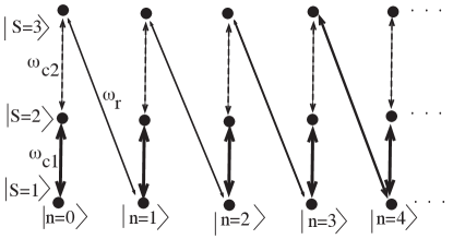
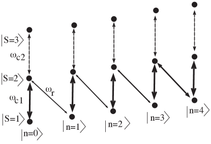
Figure 4: (a)Top: Graphical representation of the N-level ion coupled to quantum harmonic oscillator driven by sinusoidal resonant fields $\omega_{c1}$, $\omega_{c2}$ and $\omega_{r}$ as shown. The strengths of the $\omega_{c1}$ and $\omega_{c2}$ transition couplings are independent of the harmonic oscillator quantum number $n$, whereas the strengths of the $\omega_{r}$ transition couplings depend on $n$. (b) Bottom: Graphical representation of the N-level ion coupled to quantum harmonic oscillator driven by sinusoidal resonant fields $\omega_{c1}$, $\omega_{c2}$ and $\omega_{r}$ as shown. This control scheme, although not very intuitive or elegant, is based on the Finite Controllability Theorem.

Consider an additional field that accomplishes the ladder transition by connecting the $|1,n\rangle$ and the $|N,n-1\rangle$ states. In this case, the eigenstates of the coupled system are sequentially connected, and $\l_{0}$ subspace control proceeds exactly as in the previous example. The control matrices also look very similar. As before, in the interaction picture, the Schrödinger equation written as

$$\dot{Y} = (u_{1}(t)B_{c1}+u_{2}(t)B_{c2}+v(t)B_{r})Y,$$ (102)

where $u_{1,2}(t)$ and $v(t)$ are defined as before. Then qualitatively, with ‘X’, ‘Y’, ‘$Z_{i}$’s denoting non-zero, real matrix elements,

$$B_{c_{1}} = i\left(\begin{array}[]{ccc|ccc|cc}0&X&0&0&0&0&0&\ldots\\ X&0&0&0&0&0&0&\ldots\\ 0&0&0&0&0&0&0&\ldots\\ \hline\cr 0&0&0&0&X&0&0&\ldots\\ 0&0&0&X&0&0&0&\ldots\\ 0&0&0&0&0&0&0&\ldots\\ \hline\cr 0&0&0&0&0&0&0&\ldots\\ \vdots&\vdots&\vdots&\vdots&\vdots&\vdots&\vdots&\ddots\\ \end{array}\right).$$ (111)

$$B_{c_{2}} = i\left(\begin{array}[]{ccc|ccc|cc}0&0&0&0&0&0&0&\ldots\\ 0&0&Y&0&0&0&0&\ldots\\ 0&Y&0&0&0&0&0&\ldots\\ \hline\cr 0&0&0&0&0&0&0&\ldots\\ 0&0&0&0&0&Y&0&\ldots\\ 0&0&0&0&Y&0&0&\ldots\\ \hline\cr 0&0&0&0&0&0&0&\ldots\\ \vdots&\vdots&\vdots&\vdots&\vdots&\vdots&\vdots&\ddots\\ \end{array}\right).$$ (120)

$$B_{r} = \left(\begin{array}[]{ccc|ccc|cc}0&0&0&0&0&0&0&\ldots\\ 0&0&0&0&0&0&0&\ldots\\ 0&0&0&Z_{1}&0&0&0&\ldots\\ \hline\cr 0&0&-Z_{1}&0&0&0&0&\ldots\\ 0&0&0&0&0&0&0&\ldots\\ 0&0&0&0&0&0&Z_{2}&\ldots\\ \hline\cr 0&0&0&0&0&-Z_{2}&0&\ldots\\ \vdots&\vdots&\vdots&\vdots&\vdots&\vdots&\vdots&\ddots\\ \end{array}\right).$$ (129)

Another control scheme that exemplifies this theorem is an additional field that accomplishes the ladder transition by connecting the $|2,n\rangle$ and the $|N,n-1\rangle$ states, as shown in Fig. 4(b). Control in this case is a little more complicated, because the fields that transitively connect the $N$-level system must be correctly applied in order to bring the population to the $|2,n\rangle$ states before applying the ladder transition. The control matrices do not look as elegant as those in the first case, and practically this is a weaker scheme. As $N$ increases, it is clear that the number of such schemes increases. However, the sequentially connected scheme is the one that is easiest to implement. The Law-Eberly and Kneer-Law schemes can be modified to provide explicit control schemes in both these cases.

III.4 System 4: Spin-half particle coupled to two harmonic oscillators

In this section we consider another paradigm of quantum computing - the trapped-electron qubit, which can be well-modelled as a spin-half particle coupled to two harmonic oscillators. We show that this is a system that is less controllable than the spin-half particle coupled to one harmonic oscillator. In this system, it is not possible to make a transfer from any finite superposition of states to any other finite superposition. This implies in particular that the system cannot be finitely controllable. As we illustrate below, the natural control sequence does not allow one to remain within any one of the nested invariant subspaces spanned by the eigenstates. In addition the nested sequence of invariant subspaces is infinite-dimensional.

As detailed in Ref. PedersenQIP2008 , the energy eigenstates of a spin-half particle coupled to two harmonic oscillators (called the cyclotron oscillator and axial oscillator respectively) can be written as $|nlj\rangle$ where $n$ refers to the number state of the cyclotron oscillator, $l$ refers to the number state of the axial oscillator, and $j$ refers to the spin state (up or down). The system is addressed by three control fields. The spin qubit is controlled using a field of angular frequency $\omega_{s}$ that connects states $|\ n\ l\downarrow\rangle$ and $|n\ l\ \uparrow\rangle$. The spin-axial transition is controlled by field of angular frequency $\omega_{sa}$ that connects states $|n\ l\ \downarrow\rangle$ and $|n\ l+1\ \uparrow\rangle$. A spin-cyclotron transition is controlled by a field of angular frequency $\omega_{sc}$ that connects states $|n\ l\ \downarrow\rangle$ and $|n-1\ l\ \uparrow\rangle$. The transfer graph in Fig.5 clearly indicates that the three fields transitively connect all the eigenstates of the spin-axial-cyclotron system.

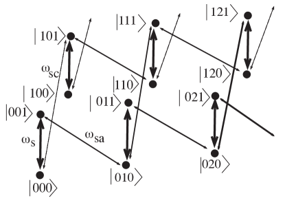
Figure 5: Transfer graph of the controlled trapped-electron. States are denoted $|nlj\rangle$, where $n$ is the cyclotron harmonic oscillator number state, $l$ is the axial harmonic oscillator number state, and $j$ is the spin state. Lines marked $\omega_{s}$, $\omega_{sa}$, and $\omega_{sc}$ indicate spin, spin-axial and spin-cyclotron transitions, respectively.

As in the case of the trapped-ion, the evolution equation is clearer in the interaction picture and is derived in Appendix References. Writing down the control matrices explicitly is not trivial, and doesn’t provide significant insights into the problem. Instead, one can look at the structure of these matrices as below. The control matrices can be written in the basis of trapped-electron eigenstates denoted by $|nlj\rangle$, where $n$ the cyclotron state, $l$ the axial state, and $j$ is the spin state. Qualitatively, S, A and C indicate spin, spin-axial and spin-cyclotron transitions, respectively, and the prefactors indicate the relative strengths. The eigenstates are ordered as: $|l=0,n=0,\downarrow\rangle,\ |l=0,n=0,\uparrow\rangle,\ |l=0,n=1,\downarrow\rangle,\ |l=0,n=1,\uparrow\rangle,\ |l=0,n=2,\downarrow\rangle,\ |l=0,n=2,\uparrow\rangle,\ \ldots,|l=1,n=0,\downarrow\rangle,\ |l=1,n=0,\uparrow\rangle,\ |l=1,n=1,\downarrow\rangle,\ |l=1,n=1,\uparrow\rangle,\ |l=1,n=2,\downarrow\rangle,\ |l=1,n=2,\uparrow\rangle,\ \ldots.$

The control matrices that describes the spin-flip and spin-axial transitions have the form

$$B_{s}=i\left[\begin{array}[]{c||c||c||c}X_{S}&0&0&\ldots\\ \hline\cr\hline\cr 0&X_{S}&0&\ldots\\ \hline\cr\hline\cr 0&0&X_{S}&\ldots\\ \hline\cr\hline\cr\vdots&\vdots&\vdots&\ddots\\ \end{array}\right],$$ (134)

$$B_{sa}=i\left[\begin{array}[]{c||c||c||c}X_{A}&0&0&\ldots\\ \hline\cr\hline\cr 0&X_{A}&0&\ldots\\ \hline\cr\hline\cr 0&0&X_{A}&\ldots\\ \hline\cr\hline\cr\vdots&\vdots&\vdots&\ddots\\ \end{array}\right],$$ (139)

respectively.

Here $X_{S}$ and $X_{A}$ are the infinite block matrices

$$X_{S}=\left[\begin{array}[]{cc|cc|cc|c}0&S&0&0&0&0&\ldots\\ S&0&0&0&0&0&\ldots\\ \hline\cr 0&0&0&S&0&0&\ldots\\ 0&0&S&0&0&0&\ldots\\ \hline\cr 0&0&0&0&0&S&\ldots\\ 0&0&0&0&S&0&\ldots\\ \hline\cr\vdots&\vdots&\vdots&\vdots&\vdots&\vdots&\ddots\\ \end{array}\right],$$ (147)

$$X_{A}=\left[\begin{array}[]{cc|cc|cc|c}0&0&0&0&0&0&\ldots\\ 0&0&A&0&0&0&\ldots\\ \hline\cr 0&A&0&0&0&0&\ldots\\ 0&0&0&0&A\sqrt{2}&0&\ldots\\ \hline\cr 0&0&0&A\sqrt{2}&0&0&\ldots\\ 0&0&0&0&0&0&\ldots\\ \hline\cr\vdots&\vdots&\vdots&\vdots&\vdots&\vdots&\ddots\\ \end{array}\right].$$ (155)

respectively.

The control matrix describing the spin-cyclotron transition has the form

$$B_{sc}=i\left[\begin{array}[]{c||c||c||c}0&X_{C}&0&\ldots\\ \hline\cr\hline\cr X_{C}^{{\dagger}}&0&X_{C}&\ldots\\ \hline\cr\hline\cr 0&X_{C}^{{\dagger}}&0&\ldots\\ \hline\cr\hline\cr\vdots&\vdots&\vdots&\ddots\\ \end{array}\right],$$ (160)

where $X_{C}$ is an infinite block matrix of the form

$$X_{C}=\left[\begin{array}[]{cc|cc|cc|c}0&C&0&0&0&0&\ldots\\ 0&0&0&0&0&0&\ldots\\ \hline\cr 0&0&0&C&0&0&\ldots\\ 0&0&0&0&0&0&\ldots\\ \hline\cr 0&0&0&0&0&C\sqrt{2}&\ldots\\ 0&0&0&0&0&0&\ldots\\ \hline\cr\vdots&\vdots&\vdots&\vdots&\vdots&\vdots&\ddots\\ \end{array}\right].$$ (168)

When the three transitions are applied sequentially, it is possible to transfer population from subspace $\mathcal{H}_{i}$ to subspace $\mathcal{H}_{i-1}$ only under certain conditions. Trivially, if one wishes to transfer population within one of the harmonic oscillator states, the problem is the same as that of the trapped ion. Also, it is easy to see that the levels are connected in such a way that the system is eigenstate controllable in the sense that the population can be coherently transferred from any eigenstate to any other eigenstate. For example, consider the set of eigenstates illustrated in Fig.5. The condition for eigenstate controllability is that the pulses of frequency $\omega_{sa}$, $\omega_{s}$ and $\omega_{sc}$ must be applied sequentially, and not simultaneously. For example, let us say we want to transfer the $|000\rangle$ state to the $|111\rangle$ state. We can do so by the pulse sequence: $p_{s}(\pi)$ that transfers to $|001\rangle$, $p_{sa}(\pi)$ that transfers to $|010\rangle$, and then $p_{sc}(\pi)$ that transfers to $|111\rangle$.

Superficially this system appears to be very similar to the trapped-ion system. However, it is seen that this system is not finitely controllable; that is, even though the system is eigenstate controllable, it is not possible to transfer a superposition of eigenstates to the ground state even with sequential applications of the field. This can be seen visually from the control graph in Fig.5, or by examining the control matrices as follows.

For example, let us say we want to transfer the $|000\rangle+|111\rangle$ state to the $|000\rangle$ state. The pulse sequence: $p_{s}(\pi)$, $p_{sa}(\pi)$, $p_{sc}(\pi)$ that transfers the $|000\rangle$ state to the $|111\rangle$ state also transfers the $|111\rangle$ state to the $|000\rangle$ state. Explicitly, $p_{s}(\pi)$ transfers $|111\rangle$ to $|110\rangle$, but also transfers $|000\rangle$ to $|001\rangle$; $p_{sa}(\pi)$ transfers $|110\rangle$ to $|101\rangle$, but also transfers $|001\rangle$ to $|010\rangle$; and $p_{sc}(\pi)$ transfers $|101\rangle$ to $|000\rangle$, but also transfers $|010\rangle$ to $|111\rangle$. The pulse sequence that transfers population down one of the harmonic oscillator ladders, transfers population up the other harmonic oscillator ladder. Thus we cannot apply the Finite Controllability Theorem using the above basis.

This lack of controllability can be attributed to the fact that the invariant subspaces are not finite-dimensional. In fact this system presents an infinite number of nested infinite -dimensional subspaces.

Thus we see that eigenstate controllability is a much weaker condition than subspace controllability. Simply having vector fields that sequentially connect the eigenstates is sufficient for eigenstate controllability. This is in contrast to the controllability of finite-dimensional quantum systems where eigenstate controllability implies controllability of finite superpositions.

This analysis provides important input into the the development of quantum gates in the trapped-electron system — it is not possible to use Law-Eberly type methods to construct arbitrary quantum gates in this system.

IV Summary

Many of the novel questions that arise in laying the ground work for quantum computing can be thought of as questions about the controllability of Schrödinger’s equation. In this paper we prove a Finite Controllability Theorem which is useful for analyzing certain infinite-dimensional quantum control problems. We discuss several related physical systems that are models for quantum computing.

Among the more interesting paradigms of quantum computing is the trapped ion modeled as a spin-half particle coupled to a quantum harmonic oscillator. In this paper, we discuss a general setting for this type of problem based on infinite-dimensional differential equations and Lie groups acting on a Hilbert space. This allows us to explore the Lie algebraic approach to controllability in this setting. In particular, we show that even though the formal Lie algebra associated with the Jaynes-Cummings model is infinite-dimensional, explicit finite controllability results can be determined. We also establish generalized controllability criteria for improving the controllability of some important infinite-dimensional quantum systems.

For the specific quantum computing system of the trapped-ion qubit, we showed that the Law-Eberly control scheme does not require the system to be in the Lamb-Dicke limit. We also showed that finite controllability cannot be achieved in the trapped-electron quantum computing paradigm, thus limiting the type of quantum operations (gates) that can be executed in this system.

Derivation of the evolution equation for the trapped-ion qubit system

The trapped-ion qubit is modeled as a spin-half particle coupled to a quantized harmonic oscillator. Since various aspects of this model are discussed in several publications, we summarize only the essential features here. Consider the description of a particle with two spin states in a quadratic potential field. The Hamiltonian now includes terms that reflect both the linear momentum of the particle in the potential field, and the spin angular momentum of the particle. The Schrödinger equation can be written as a two-component vector equation

$$\left[\begin{array}[]{c}\frac{\partial\psi_{+}}{\partial t}\\ \frac{\partial\psi_{-}}{\partial t}\end{array}\right] = \frac{i}{2}\left[\begin{array}[]{cc}\Omega_{m}-\omega_{0}&0\\ 0&\Omega_{m}+\omega_{0}\end{array}\right]\left[\begin{array}[]{c}\psi_{+}\\ \psi_{-}\end{array}\right]$$ (175)

where $\Omega_{m}=\omega_{m}\left(\frac{\partial^{2}}{\partial x^{2}}-x^{2}\right)$. The subscripts $+$ and $-$ refer to the two levels of the atom (modelled in physics literature as the spin-up and spin-down states of a spin-$1/2$ particle). An applied field causes transitions between the eigenstates of the coupled spin-oscillator system.

In order to understand the control of this system, we briefly present the a spin-$0$ particle in a quadratic potential with resonant frequency $\omega_{m}$ being excited by a traveling wave of central frequency $\omega$ with controllable amplitude $E(t)$. This system might be described by an equation of the form

$$\frac{\partial\psi}{\partial t}=\frac{i\omega_{m}}{2}\left(\frac{\partial^{2}}{\partial x^{2}}-x^{2}\right)\psi-iE(t)\mu\cos(kx-\omega t)\psi,$$ (176)

where $\mu$ is a dipole operator that describes the transition couplings between various eigenstates of the system, and $k$ is the wavevector of the applied field. Let us introduce the differential operators

$$a=\frac{1}{\sqrt{2}}\left(x+\frac{\partial}{\partial x}\right),$$ (177)

and

$$a^{\dagger}=\frac{1}{\sqrt{2}}\left(x-\frac{\partial}{\partial x}\right).$$ (178)

These are the familiar creation and annihilation operators of the quantized harmonic oscillator [35]. Introducing the differential operators corresponding the position of the particle in the harmonic potential, and using the notation established in the previous subsection, Eq. 176 becomes

$$\frac{\partial\psi}{\partial t} = -i\omega_{m}\left(N+\frac{1}{2}\right)\psi$$ (179)

$$-i\left(E(t)\mu\cos(\omega t-kx_{0}(a+a^{\dagger})\right)\psi.$$

The product of $k$, the wavelength of the light, and $x_{0}$, the amplitude of the zero-point motion of the particle in the harmonic potential (or the spatial extent of the ground state harmonic oscillator wave function) is the Lamb-Dicke parameter $\eta$. Recall that the driving field is not resonant with the characteristic frequency of the harmonic potential. Therefore the above equation can be simplified only with the knowledge of the driving frequency, and the matrix elements of the operator $\mu$ that can be coupled by that driving frequency due to energy conservation.

Returning to the system described by Eq. 175, an applied field causes transitions between the eigenstates of the coupled spin-oscillator system. The amplitudes corresponding to the fields that cause the carrier and red transitions are dubbed $E_{c}$ and $E_{r}$ respectively. When both fields are applied simultaneously, ignoring overall additive constants, the control equations take on the form

$$\left[\begin{array}[]{c}\frac{\partial\psi_{+}}{\partial t}\\ \frac{\partial\psi_{-}}{\partial t}\end{array}\right]=\frac{i}{2}\left[\begin{array}[]{cc}\Omega_{m}-\omega_{0}&0\\ 0&\Omega_{m}+\omega_{0}\end{array}\right]\left[\begin{array}[]{c}\psi_{+}\\ \psi_{-}\end{array}\right]$$ (186)

$$-i\left[\begin{array}[]{cc}0&\mu_{c}E_{c}(t)+\mu_{r}E_{r}(t)\\ \mu_{c}E_{c}(t)+\mu_{r}E_{r}(t)&0\end{array}\right]\left[\begin{array}[]{c}\psi_{+}\\ \psi_{-}\end{array}\right];$$ (191)

where, $\mu_{c,r}$ is short for $\mu\cos(\omega_{c,r}t-\eta(a+a^{\dagger}))$. Here $\mu$ is the dipole operator that describe the strengths of the transitions between the two-level system eigenstates coupled by the fields. Examining the cosine terms in the off-diagonals, these can be expanded as

$$\cos(\omega t-\eta(a+a^{\dagger}))= \frac{1}{2}\left(\exp(i\omega t)\exp(-i\eta(a+a^{\dagger})))\right.$$

$$+\left.\exp(-i\omega t)\exp(i\eta(a+a^{\dagger})))\right).$$

Thinking in terms of the field adding energy to the ionic state (two level system), the term $\exp(-i\omega t)$ adds energy $\hbar\omega$ to a state while the term $\exp(i\omega t)$ removes energy $\hbar\omega$ from a state. For a true two-level system, one cannot add energy to the excited state, nor remove energy from the ground state. So, keeping only the energy conserving terms (rotating wave approximation), the control equations become

$$\left[\begin{array}[]{c}\frac{\partial\psi_{+}}{\partial t}\\ \frac{\partial\psi_{-}}{\partial t}\end{array}\right] = \frac{i}{2}\left[\begin{array}[]{cc}\Omega_{m}-\omega_{0}&0\\ 0&\Omega_{m}+\omega_{0}\end{array}\right]\left[\begin{array}[]{c}\psi_{+}\\ \psi_{-}\end{array}\right]$$ (209)

$$-iE_{c}\left[\begin{array}[]{cc}0&\tilde{\mu}_{c}\\ \tilde{\mu}_{c}^{*}&0\end{array}\right]\left[\begin{array}[]{c}\psi_{+}\\ \psi_{-}\end{array}\right]$$

$$-iE_{r}\left[\begin{array}[]{cc}0&\tilde{\mu}_{r}\\ \tilde{\mu}_{r}^{*}&0\end{array}\right]\left[\begin{array}[]{c}\psi_{+}\\ \psi_{-}\end{array}\right].$$

where $\tilde{\mu}_{c,r}$ is short for $\mu\exp(-i\omega_{c,r}t+i\eta(a+a^{\dagger}))$.

In order to write the evolution equation in matrix form, the eigenstates are ordered as $|\uparrow,0\rangle,\ |\uparrow,1\rangle,\ \ldots,|\downarrow,0\rangle,\ |\downarrow,1\rangle,\ \ldots$. The drift matrix of this system can be written in block matrix form as:

$$-i\left(\begin{array}[]{c|c}\frac{\omega_{0}}{2}+N\omega_{m}&0\\ \hline\cr 0&\frac{-\omega_{0}}{2}+N\omega_{m}\\ \end{array}\right),$$ (212)

where, $N$ is the previously defined number operator. The control matrices are not easily expressed in this basis.

The evolution equation takes on a much simpler and elegant form in the interaction picture. Also, the transition matrices are described compactly by using the three Pauli matrices $\sigma_{x}$, $\sigma_{y}$, and $\sigma_{z}$. For example, the spin-flip transition is described by the operator $\sigma_{+}=\sigma_{x}+i\sigma_{y}$ and its hermitian conjugate $\sigma_{-}$. In a coordinate system defined by the eigenbasis of the coupled system ($|S,n\rangle$, where $S$ refers to the spin state and $n$ to the harmonic oscillator number state), a general matrix element of the control Hamiltonian $\langle S^{\prime}n^{\prime}|H_{I}^{\prime}|Sn\rangle$ may be written as [17, 43]:

$$-i2{\rm Re}\left[\langle S^{\prime}|\sigma_{+}|S\rangle\langle n^{\prime}|\exp(i(\eta(a+a^{{\dagger}})))|n\rangle\right]$$

$$=-i2{\rm Re}\left[\langle S^{\prime}|\sigma_{+}|S\rangle\exp(-\eta/2)\sqrt{\frac{n_{<}!}{n_{>}!}}\ (i\eta)^{|n^{\prime}-n|}L_{n<}^{|n^{\prime}-n|}(\eta^{2})\right].\quad$$

The symbol $n_{>}$ refers to the larger of $n$ and $n^{\prime}$, and $n_{<}$ refers to the smaller of $n$ and $n^{\prime}$. Here $L_{n}^{\alpha}(x)$ is the associated Laguerre polynomial. When the applied field of frequency $\omega_{c}$ connects states $|\downarrow,n\rangle$ and $|\uparrow,n\rangle$ (carrier transitions), $n^{\prime}=n$, and when the applied field of frequency $\omega_{r}$ connects states $|\downarrow,n\rangle$ and $|\uparrow,n-1\rangle$ (red sideband transitions), $n^{\prime}=n-1$. The matrix elements are zero for all other values of $n^{\prime}$.

Derivation of the evolution equation for the trapped-electron qubit system

We consider a trapped-electron qubit which can be well-modelled as a spin-half particle coupled to two harmonic oscillators. As detailed in Ref. [46], the relevant quantum states are the spin states of the electron (a spin-half particle), and the harmonic oscillator number states of the cyclotron and axial harmonic potentials. As before, the evolution is described by

$$\left[\begin{array}[]{c}\frac{\partial\psi_{+}}{\partial t}\\ \frac{\partial\psi_{-}}{\partial t}\end{array}\right] = -\frac{i}{2}\left[\begin{array}[]{cc}\Omega_{tot}&0\\ 0&\Omega_{tot}\end{array}\right]\left[\begin{array}[]{c}\psi_{+}\\ \psi_{-}\end{array}\right];$$ (219)

where $\Omega_{tot}=\omega_{c}\left(-\frac{\partial^{2}}{\partial x_{c}^{2}}+\beta x_{c}^{2}\right)+\omega_{z}\left(-\frac{\partial^{2}}{\partial x_{z}^{2}}+x_{z}^{2}\right)+\omega_{s}$. Here, $\omega_{s}$ refers to the angular frequency associated with the spin-flip of the electron. The parameter $\beta$ indicates that the cyclotron harmonic potential (indicated by subscript $c$) and the axial harmonic potential (indicated by subscript $z$) are of different strengths.

In the basis of the harmonic oscillator eigenstates, the drift matrix can be written as

$$\left[\begin{array}[]{cc}\omega^{\prime}_{c}N_{c}+\omega_{z}N_{z}+\frac{\omega_{s}}{2}&0\\ 0&\omega^{\prime}_{c}N_{c}+\omega_{z}N_{z}-\frac{\omega_{s}}{2}\end{array}\right],$$ (222)

where the frequencies $\omega_{c}$ and $\omega_{z}$ refer to the frequencies of the cyclotron and axial harmonic oscillators, and $\omega_{s}$ refers to the spin flip transition frequency.

The energy eigenstates can be written as $|nlj\rangle$ where $n$ refers to the number state of the cyclotron oscillator, $l$ refers to the number state of the axial oscillator, and $j$ refers to the spin state (up or down). The system is addressed by three control fields. The spin qubit is controlled using a small transverse magnetic field that connects states $|\ n\ l\downarrow\rangle$ and $|n\ l\ \uparrow\rangle$. The spin-axial transition is controlled by a travelling magnetic field that connects states $|n\ l\ \downarrow\rangle$ and $|n\ l+1\ \uparrow\rangle$. A spin-cyclotron transition is controlled by an oscillating magnetic field with a spatial gradient that connects states $|n\ l\ \downarrow\rangle$ and $|n-1\ l\ \uparrow\rangle$. The transfer graph in Fig.5 clearly indicates that the three fields transitively connect all the eigenstates of the spin-axial-cyclotron system.

As in the case of the trapped-ion, the evolution equation is clearer in the interaction picture. The evolution equation is given by

$$\dot{Z} = (\Omega_{s}(t)B_{s}+\Omega_{sa}(t)B_{sa}+\Omega_{sc}(t)B_{sc})Z.$$ (223)

Here $\Omega_{s}(t)$ is the control parameter for the spin flip transition, $\Omega_{sz}(t)$ is the control parameter for the spin axial transition, and $\Omega_{sc}(t)$ is the control parameter for the spin cyclotron transition. The spin-flip transition operator $B_{s}=-i/2\left(\sigma_{+}\exp(-i\phi)+\sigma_{-}\exp(i\phi)\right)$. The spin-axial transition operator

$$\begin{split}B_{sa}=&-i\bigl{(}\sigma_{+}\exp(i(\eta(a^{\dagger}_{z}e^{i\omega_{z}t}+a_{z}e^{-i\omega_{z}t})-\Delta\cdot t-\phi))\\ &+\sigma_{-}\exp(-i(\eta(a^{\dagger}_{z}e^{i\omega_{z}t}+a_{z}e^{-i\omega_{z}t})-\Delta\cdot t-\phi))\bigr{)}\end{split}$$ (224)

where the characteristic frequency of the transition is $\omega_{sa}=\omega_{s}+\omega_{z}$, the detuning $\Delta=\omega-\omega_{s}$, $\phi$ is an experimentally variable phase, and $\eta$ is the Lamb-Dicke parameter. Here $a_{z}$ and $a^{\dagger}_{z}$ are annhilation and creation operators respectively associated with the axial harmonic oscillator. For $\omega=\omega_{sa}$ (when the applied field is at resonance with the spin-axial transition) only the levels $|\!nl\!\downarrow\rangle$ and $|\!n(l+1)\!\uparrow\rangle$ are connected. The spin-cyclotron transition operator $B_{sc}=-i(\sigma_{+}a_{c}e^{-i\phi}+\sigma_{-}a_{c}^{\dagger}e^{i\phi})$, where $\omega_{sc}=\omega_{s}-\omega^{\prime}_{c}$ is the characteristic frequency associated with the spin cyclotron transition. Here $a_{c}$ and $a^{\dagger}_{c}$ are annhilation and creation operators respectively associated with the cyclotron harmonic oscillator. When the applied field is in resonance with the spin-cyclotron transition $\omega=\omega_{sc}$, only the levels $|\!nl\!\downarrow\rangle$, $|\!(n-1)l\uparrow\rangle$ are connected.

References

- [1] GM Huang, TJ Tarn, and JW Clark. On the controllability of quantum-mechanical systems. Journal of Mathematical Physics, 24(11):2608–2618, 1983.
- [2] M Shapiro and P Brumer. Laser control of product quantum state populations in unimolecular reactions. Journal of Chemical Physics, 84(7):4103–4104, 1986.
- [3] DJ Tannor, R Kosloff, and SA Rice. Coherent pulse sequence induced control of selectivity of reactions - Exact quantum-mechanical calculations. Journal of Chemical Physics, 85(10):5805–5820, 1986.
- [4] DJ Tannor and SA Rice. Control of selectivity of chemical-reaction via control of wave packet evolution. Journal of Chemical Physics, 83(10):5013–5018, 1985.
- [5] AP Peirce, MA Dahleh, and H Rabitz. Optimal-control of quantum-mechanical systems - existence, numerical approximation, and applications. Physical Review A, 37(12):4950–4964, 1988.
- [6] C Rangan and PH Bucksbaum. Optimally shaped terahertz pulses for phase retrieval in a Rydberg-atom data register. Physical Review A, 6403(3), 2001.
- [7] JP Palao and R Kosloff. Quantum computing by an optimal control algorithm for unitary transformations. Physical Review Letters, 89(18), 2002.
- [8] KR Brown, J Vala, and KB Whaley. Scalable ion trap quantum computation in decoherence-free subspaces with pairwise interactions only. Physical Review A, 67(1), 2003.
- [9] N Khaneja, R Brockett, and SJ Glaser. Time optimal control in spin systems. Physical Review A, 6303(3), MAR 2001.
- [10] EA Shapiro, M Spanner, and MY Ivanov. Quantum logic approach to wave packet control. Physical Review Letters, 91(23), 2003.
- [11] Kurt Jacobs. Engineering Quantum States of a Nanoresonator via a Simple Auxiliary System. Physical Review Letters, 99(11), 2007.
- [12] See articles in. Implementations of Quantum Computing. Quantum Information and Computation, 1, 2001.
- [13] CK Law and JH Eberly. Arbitrary control of a quantum electromagnetic field. Physical Review Letters, 76(7):1055–1058, 1996.
- [14] B Kneer and CK Law. Preparation of arbitrary entangled quantum states of a trapped ion. Physical Review A, 57(3):2096–2104, 1998.
- [15] A. Ben-Kish et al. Experimental demonstration of a technique to generate arbitrary quantum superposition states of a harmonically bound spin-1/2 particle. Physical Review Letters, 90(3), 2003.
- [16] RW Brockett, C Rangan, and AM Bloch. The controllability of infinite quantum systems. Proceedings of the 42nd IEEE Conference on Decision and Control, pages 428–433, 2003.
- [17] C Rangan, AM Bloch, C Monroe, and PH Bucksbaum. Control of trapped-ion quantum states with optical pulses. Physical Review Letters, 92(11), 2004.
- [18] C Rangan and AM Bloch. Control of finite-dimensional quantum systems: Application to a spin-1/2 particle coupled with a finite quantum harmonic oscillator. Journal of Mathematical Physics, 46(3), 2005.
- [19] RW Brockett. System theory on group manifolds and coset spaces. SIAM Journal on Control, 10(2):265–&, 1972.
- [20] RW Brockett. Lie theory and control-systems defined on spheres. SIAM Journal on Applied Mathematics, 25(2):213–225, 1973.
- [21] V Ramakrishna, MV Salapaka, M Dahleh, H Rabitz, and A Peirce. Controllability of molecular-systems. Physical Review A, 51(2):960–966, 1995.
- [22] F Albertini and D D’Alessandro. Notions of controllability for bilinear multilevel quantum systems. IEEE Transactions on Automatic Control, 48(8):1399–1403, 2003.
- [23] E. Zuazua. Remarks on the controllability of the Schrödinger equation. Proc. CRM., Montreal, pages 1–17, 2000.
- [24] Gabriel Turinici and Herschel Rabitz. Wavefunction controllability in quantum systems. Journal of Physics A, 36():2565–2576, 2003.
- [25] JM Ball, JE Marsden, and M Slemrod. Controllability for distributed bilinear-systems. SIAM Journal on Control and Optimization, 20(4):575–597, 1982.
- [26] K Beauchard. Local controllability of a 1-D Schrödinger equation. J. Math. Pures et Appl., 84:851–956, 2005.
- [27] Reinhard Illner, Horst Lange, and Holger Teismann. Limitations on the control of Schr dinger equations. ESAIM: COCV, 12():615–635, 2006.
- [28] G Turinici. Controllable quantities for bilinear quantum systems. Proceedings of the 39th IEEE Conference on Decision and Control, pages 1364–1369, 2000.
- [29] EA Shapiro, MY Ivanov, and Y Billig. Coarse-grained controllability of wavepackets by free evolution and phase shifts. Journal of Chemical Physics, 120(21):9925–9933, 2004.
- [30] W Karwowski and RV Mendes. Quantum control in infinite dimensions. Physics Letters A, 322(5-6):282–285, 2004.
- [31] CH Lan, TJ Tarn, QS Chi, and JW Clark. Analytic controllability of time-dependent quantum control systems. Journal of Mathematical Physics, 46(5), 2005.
- [32] R. Adami and U. Boscain. Controllability of the Schroedinger Equation via Intersection of Eigenvalues. Proceedings of the 44rd IEEE Conference on Decision and Control, 2005.
- [33] RB Wu, TJ Tarn, and CW Li. Smooth controllability of infinite-dimensional quantum-mechanical systems. Physical Review A, 73(1), 2006.
- [34] T. Chambrion, P. Mason, M. Sigalotti, and U. Boscain. Controllability of the discrete-spectrum Schroedinger equation driven by an external field. Annales de l’Institut Henri Poincare (C) Non Linear Analysis, 26(1):329–349, 2009.
- [35] Leonard I. Schiff. Quantum Mechanics. McGraw-Hill, New York, 1968.
- [36] M Mirrahimi and P Rouchon. Controllability of quantum harmonic oscillators. IEEE Transactions on Automatic Control, 49(5):745–747, 2004.
- [37] Bruce W. Shore. Theory of Coherent Atomic Excitation, Volume 2, Multilevel Atoms and Incoherence. Wiley-VCH, 1990.
- [38] S Lloyd and SL Braunstein. Quantum computation over continuous variables. Physical Review Letters, 82(8):1784–1787, 1999.
- [39] Neilson Dunford and Jacob T. Schwartz. Linear operators, General Theory (Part I). Wiley-Interscience, 1988.
- [40] K Kime. Control of transition-probabilities of the quantum-mechanical harmonic-oscillator. Applied Mathematics Letters, 6(3):11–15, 1993.
- [41] A.R.P. Rau and Unnikrishnan. Unitary integration of time-dependent Schrodinger equation. Physics Letters A, 222:304–308, 1996.
- [42] Roy J. Glauber. Coherent and incoherent states of the radiation field. Physical Review, 131(6):2766–2788, 1963.
- [43] DJ Wineland, C Monroe, WM Itano, D Leibfried, BE King, and DM Meekhof. Experimental issues in coherent quantum-state manipulation of trapped atomic ions. Journal of Research of the National Institute of Standards and Technology, 103(3):259–328, 1998.
- [44] ET Jaynes and FW Cummings. Comparison of quantum and semiclassical radiation theories with application to beam maser. Proceedings of the IEEE, 51(1):89, 1963.
- [45] G Turinici. Exact controllability for the population of the eigenstates in bilinear quantum systems. Comptes Rendus de l Academie des Sciences Serie I-Mathematique, 330(4):327–332, 2000.
- [46] LH Pedersen and C Rangan. Controllability and universal three-qubit quantum computation with trapped electron states. Quantum Information Processing, 7:33–42, 2008.