Quantum phase transitions and quantum fidelity
in free fermion graphs

Abstract

In this paper we analyze the ground state phase diagram of a class of fermionic Hamiltonians by looking at the fidelity of ground states corresponding to slightly different Hamiltonian parameters. The Hamiltonians under investigation can be considered as the variable range generalization of the fermionic Hamiltonian obtained by the Jordan-Wigner transformation of the XY spin-chain in a transverse magnetic field. Under periodic boundary conditions, the matrices of the problem become circulant and the models are exactly solvable. Their free-ends counterparts are instead analyzed numerically. In particular, we focus on the long range model corresponding to a fully connected directed graph, providing asymptotic results in the thermodynamic limit, as well as the finite-size scaling analysis of the second order quantum phase transitions of the system. A strict relation between fidelity and single particle spectrum is demonstrated, and a peculiar gapful transition due to the long range nature of the coupling is found. A comparison between fidelity and another transition marker borrowed from quantum information i.e., single site entanglement, is also considered.

I Introduction

In the last years, several papers have shown that the study of quantum phase transitions (QPTs) can benefit from the application of concepts borrowed from quantum information theory. In particular, the behavior of entanglement at quantum critical points, due to its connection with quantum correlations, typically presents peculiar features which can be used as transition markers, thereby providing further insight into these phenomena entanglement . More recently, QPTs have also been analyzed from the point of view of Berry’s geometric phase geometric , a quantity which has in fact been found to contribute to entanglement entropy ryu06 .

One of the most recent reasons of interest in quantum phase transitions for the quantum information community is the relationship between criticality and decoherence decoherence . Another relevant aspect is connected with adiabatic quantum computing aqc , as the proximity to QPTs could cause the failure of adiabaticity conditions. On the other hand, crossing of QPTs could be desirable to transform easy-to-prepare states into non-trivial states corresponding to the solution of computationally relevant problems. Transitions with non-vanishing energy gap, like topological QPTs, could allow such an implementation of adiabatic algorithms and therefore the achievement of significant computational speedups topological .

In Refs. za-pa ; za-co-gio an approach to quantum phase transitions in terms of ground state fidelity (the overlap modulus) was proposed. In practice, this consists in analyzing the fidelity between ground states corresponding to slightly different Hamiltonian parameters. The intuitive idea underlying this method is that in the proximity of critical regions a small change of the Hamiltonian parameters can give rise to dramatic ground state (GS) variations, due to the strong difference of the GS structure in opposite phases. The overlap between neighboring states is then expected to decrease abruptly at the phase boundaries. In Ref. za-pa this idea was successfully applied to the study of the Dicke and XY models, where a one to one correspondence was found between the sudden drops of the overlap function and the critical points of the phase diagram. In Ref. za-co-gio a more extensive analysis on general free Fermi systems was presented, providing a description of the fidelity features in terms of the matrices of coupling constant entering the system Hamiltonian. In particular, explicit connections between the vanishing of the lowest single particle energy (the gap) and the fidelity drops were shown. An exemplification of these concepts in a model corresponding to a totally connected fermionic graph was also included.

In this article we further develop the general formalism presented in Ref. za-co-gio , deriving in detail and expanding some of the results reported there. In particular, we characterize the fidelity behavior by a proper combination $h$ of its second derivatives, namely the lowest eigenvalue of the Hessian matrix. Furthermore, we describe a class of exactly solvable models which offer the ideal playground for the study of the relations between ground state fidelity and QPTs. The corresponding Hamiltonians are the cyclic variable range generalization of the fermionic Hamiltonian obtained by the Jordan-Wigner transformation of the XY spin-chain in a transverse magnetic field. We also consider their free-ends counterparts, which are however analyzed numerically, as the analytical results available for the cyclic case make crucially use of the simple properties of the circulant matrices appearing in the presence of periodic boundary conditions. We then focus on the long range model corresponding to a fully connected fermionic graph. Along with some first order QPTs, two second order QPTs are found, as anticipated in Ref. za-co-gio for the free-ends case. One of them is an example of a gapful second order QPT, an uncommon situation also found in topological QPTs. The existence of a transition in the absence of a vanishing single particle energy turns out here to be due to the (unphysical) long range nature of the coupling. In order to ascertain the second order nature of such transition, in the analytical cyclic case we also study the ground state energy derivatives, finding explicitly a discontinuity at the phase boundary in the thermodynamic limit (TDL). Furthermore, the finite-size scaling behavior typical of second order transitions is recovered in the function $h$. Finally, we calculate the single-site entanglement and compare its behavior with that of fidelity in critical regions.

The paper is organized as follows. In Sec. II we review and discuss in more detail the general results on quadratic fermionic Hamiltonians already presented in Ref. za-co-gio . In particular, after a brief summary of the diagonalization procedure of Ref. lieb61 , Subsec. II.1 is devoted to the general expression of the GS in these systems, Subsec. II.2 to the explicit calculation of the fidelity, and Subsec. II.3 to fidelity derivatives and the function $h$. In Sec. III we introduce the class of variable range models we have developed. We begin by recalling the fermionic Hamiltonian obtained by the Jordan-Wigner transformation of the XY spin-chain in a transverse magnetic field, which motivated the introduction of our models, and then provide the analytical solution for the variable range cyclic case. In Sec. IV the long range fully coordinated system is described in detail, first providing an exhaustive analytic description of the cyclic graph (Subsec. IV.1) and then presenting the numerical results obtained for the free-ends one (Subsec. IV.2). In this section all the formalism developed in Sec. I for the fidelity approach is concretely applied to the study of the phase diagram of the system. The finite-size scaling of $h$ in the neighborhood of second order QPTs and its asymptotic behavior in the thermodynamic limit are discussed, along with the GS energy. Then, in Sec. V we report our results on single-site entanglement, whose behavior in critical regions also shows transition signatures. Finally, we draw our conclusions in Sec. VI. Some technical details can be found in the Appendices.

II Ground state fidelity in quadratic fermionic Hamiltonians

The most general quadratic Hamiltonian describing a system of $L$ free fermionic modes is given by

$$H=\sum_{i,j=1}^{L}c_{i}^{\dagger}A_{ij}c_{j}+\frac{1}{2}\sum_{i,j=1}^{L}(c_{i}^{\dagger}B_{ij}c_{j}^{\dagger}+\mathrm{h.c.})\ ,$$ (1)

where $c_{i}$, $c_{i}^{\dagger}$ are the annihilation and creation operators of the $i$-th mode and the matrices $A$, $B$ are hermitian and skew-symmetric respectively, due to the hermiticity of $H$ and the anticommutation properties of the fermionic operators. In the following, we restrict ourselves to the case where $A$ and $B$ are real matrices. The generality of the system described by Eq. (1) can then be appreciated by representing $A$ and $B$ in terms of the generic (real) matrix $Z$, i.e., $A\equiv(Z^{T}+Z)/2$ and $B\equiv(Z^{T}-Z)/2$. This allows to identify the space of coupling constants of Eq. (1) with the $L^{2}$-dimensional full matrix algebra $M_{L}({\mathrm{I\!R}})$. Correspondingly, as it will be illustrated below, the system’s ground state properties and their changes in the presence of QPTs will be completely characterized by the matrix $Z$, which is hence of fundamental importance in our description.

The above Hamiltonian can be rewritten in the more compact form $H=(\bm{\Psi}^{\dagger}C\bm{\Psi}+\text{Tr}\,A)/2$, where $\bm{\Psi}=(c_{1},\dots,c_{L},c_{1}^{\dagger},\dots,c_{L}^{\dagger})^{T}$, $\bm{\Psi}^{\dagger}=(c_{1}^{\dagger},\dots,c_{L}^{\dagger},c_{1},\dots,c_{L})$, and $C=\sigma_{z}\otimes{}A+i\sigma_{y}\otimes{}B$. This notation, also used in Ref. rossini06 , will be adopted throughout this section.

The diagonalization problem for Eq. (1) has been solved in Ref. lieb61 . This well known procedure is very powerful, as it involves operations in the parameter space of dimension $L^{2}$, instead of in the full Hilbert space of the system, which has dimension $2^{L}$. Below, we derive the results of Ref. lieb61 by making use of the general properties of real canonical transformations, which we briefly recall also in view of some simple applications in the next Subsection.

Real canonical transformations – We consider the linear transformation

$$c_{j}^{\prime}=\sum_{k=1}^{L}(u_{jk}c_{k}+v_{jk}c_{k}^{\dagger})\ ,$$ (2)

where $u$, $v$ are real matrices. Correspondingly, $\bm{\Psi}^{\prime}=V\bm{\Psi}$, where $V=\openone_{2}\otimes{}u+\sigma_{x}\otimes{}v$ and the subscript is used to specify the dimension of the unit matrix whenever different from $L$. The transformation is canonical if it preserves the anticommutation relations. This implies $V$ to be orthogonal, i.e., the canonical conditions

$$uu^{T}+vv^{T}=\openone\ ,$$ (3a)

$$uv^{T}+(uv^{T})^{T}=\mathbb{0}\ .$$ (3b)

The Hamiltonian becomes $H=({\bm{\Psi}^{\prime}}^{\dagger}{}C^{\prime}\bm{\Psi}^{\prime}+\mathrm{Tr}A)/2$, where $C^{\prime}=VCV^{T}=\sigma_{z}\otimes{}A^{\prime}+i\sigma_{y}\otimes{}B^{\prime}$. Apart from the constant energy shift, which is still given by $\mathrm{Tr}A/2$, the structure of $H$ is then preserved in terms of the primed quantities. One can thus define $Z^{\prime}=A^{\prime}-B^{\prime}$, therefore finding by straightforward calculations the simple relation

$$Z^{\prime}=(u+v)Z(u-v)^{T}\ .$$ (4)

Hamiltonian diagonalization – For the diagonalization of Eq. (1) one then needs to diagonalize the $2L\times 2L$ symmetric matrix $C$, i.e., $C=V^{T}C^{\prime}V$ with $C^{\prime}$ diagonal. We note that the eigenvalue matrix $C^{\prime}$ can always be written in the form $C^{\prime}=\sigma_{z}\otimes\Lambda$, where the $L\times{}L$ diagonal matrix $\Lambda=\mathrm{diag}(\Lambda_{1},\dots,\Lambda_{L})$ is positive semi-definite. Indeed, it is easy to see that $\det(C-c\openone_{2L})=0$ imposes $\det(C+c\openone_{2L})=0$ as well, i.e., the eigenvalues of the symmetric matrix $C$ appear in pairs of real numbers of opposite sign. On the other hand, one also has $C^{\prime}=\sigma_{z}\otimes{}A^{\prime}+i\sigma_{y}\otimes{}B^{\prime}$, so that $A^{\prime}=\Lambda$, $B^{\prime}=0$ and hence $Z^{\prime}=\Lambda$. From Eq. (4), by defining $\Phi\equiv{}u+v$ and $\Psi\equiv{}u-v$, one finally gets the important equation

$$\Phi{}Z\Psi^{T}=\Lambda\ ,$$ (5)

also implying $\Psi{}Z^{T}\Phi^{T}=\Lambda$. Note that, due to the canonical conditions (3) obeyed by $u$ and $v$, the matrices $\Phi$ and $\Psi$ must be orthogonal. It is then straightforward to derive the further relations $\Lambda\Psi=\Phi{}Z$, $\Lambda\Phi=\Psi{}Z^{T}$ and $\Phi{}ZZ^{T}=\Lambda^{2}\Phi$, $\Psi{}Z^{T}Z=\Lambda^{2}\Psi$. In practice, one can for example solve $\Phi{}ZZ^{T}=\Lambda^{2}\Phi$ for $\Phi$ and $\Lambda$, and then obtain $\Psi=\Lambda^{-1}\Phi{}Z$. Whenever $\Lambda_{j}=0$, the equation $\Lambda\Psi=\Phi{}Z$ cannot be completely solved for $\Psi$, but one can recover the $j$-th row of $\Psi$ from $\Lambda\Phi=\Psi{}Z^{T}$. Alternatively, one first solves for $\Psi$ and $\Lambda$, and then for $\Phi$. Clearly, due to Eq. (5), $\Phi$ and $\Psi$ are not independent, so that in general they cannot be calculated by diagonalizing $ZZ^{T}$ and $Z^{T}Z$ separately.

In conclusion, after solving Eq. (5) for $\Phi$, $\Psi$ orthogonal and $\Lambda$ diagonal, one introduces $g\equiv(\Phi+\Psi)/2$ and $h\equiv(\Phi-\Psi)/2$, in terms of which the canonically transformed operators diagonalizing the Hamiltonian are defined by $\eta_{j}\equiv\sum_{k=1}^{L}(g_{jk}c_{k}+h_{jk}c_{k}^{\dagger})$. The Hamiltonian finally reads

$$H=\sum_{j=1}^{L}\Lambda_{j}\eta_{j}^{\dagger}\eta_{j}+E_{0}\ ,$$ (6)

where $E_{0}=\mathrm{Tr}(A-\Lambda)/2$ is the ground state energy and the $\Lambda_{i}$’s are found to play the role of single particle energies.

II.1 Ground State

In this subsection we present the explicit expression of the ground state of Eq. (1), starting from the Ansatz of Ref. peschel . The Hamiltonian, although not number conserving due to the terms containing the antisymmetric matrix $B$, preserves the number parity $P_{N}=(-1)^{N}$, where $N=\sum_{j=1}^{L}c_{j}^{\dagger}{}c_{j}$ is the fermion number operator. In formulas, $[H,N]\neq 0$ and $[H,P_{N}]=0$. Hence, the ground state must be a superposition of states with even or odd number of fermions exclusively. In the case of even parity, it can be of the following form peschel

$$|\Psi_{Z}\rangle=\mathcal{N}\exp\left(\frac{1}{2}\sum_{j,k=1}^{L}c_{j}^{\dagger}G_{jk}c_{k}^{\dagger}\right)|0\rangle\ ,$$ (7)

where $\mathcal{N}$ is the normalization factor, $|0\rangle$ is the fermionic vacuum ($c_{i}|0\rangle=0$) and $G$ is a real $L\times L$ antisymmetric matrix. The link with the above diagonalization procedure can be made by imposing the ground state condition $\eta_{k}|\Psi_{Z}\rangle=0,\;\forall\;k$ peschel . Then, the matrix $G$ must be the solution of the equation

$$gG+h=0\ ,$$ (8)

where it is worth recalling $g=(\Phi+\Psi)/2$ and $h=(\Phi-\Psi)/2$. Note that the latter equation is not always solvable, corresponding to cases where either the Ansatz (7) does not hold or the ground state parity is odd. We will return on this point below.

The bridge with the picture of the previous subsection can be made more stringent whenever $\Lambda$ (and hence $Z$) is invertible. In fact, by using Eq. (5) one can write $g=\Phi(\openone+\Lambda_{\Phi}^{-1}Z)/2$, $h=\Phi(\openone-\Lambda_{\Phi}^{-1}Z)/2$, with $\Lambda_{\Phi}\equiv\Phi^{-1}\Lambda\Phi$, so that if $g$ is invertible one has

$$G=\frac{T-\openone}{T+\openone}\ ,$$ (9)

where $G$ is now seen as the Cayley transform of $T\equiv\Lambda_{\Phi}^{-1}Z$ bathia . The fraction symbol is here not ambiguous, as we are dealing with commuting matrices, $[T-\openone,(T+\openone)^{-1}]=[T+\openone-2\cdot\openone,(T+\openone)^{-1}]=0$. The matrix $T\equiv\Lambda_{\Phi}^{-1}Z$ can be seen as the orthogonal part of the polar decomposition of $Z$. The latter is the generalization to matrices of the polar decomposition of a complex number $z=|z|e^{i\arg{z}}$. For a generic matrix $M$ one can write $M=PU$, with $U$ unitary and $P=\sqrt{MM^{\dagger}}$ positive semidefinite (note that $\det{M}=pe^{i\theta}$, with $p=|\det{M}|$ and $e^{i\theta}=\det{U}$). If $M$ is normal, $[M,M^{\dagger}]=0$, then one can use without ambiguity the notation $|M|=\sqrt{MM^{\dagger}}=\sqrt{M^{\dagger}{}M}$. In our case, from Eq. (5) we immediately obtain the relation $P^{2}=ZZ^{T}=\Lambda_{\Phi}^{2}$ and thus $U=T=\Phi^{T}\Psi$, real. Note that, from Eq. (9), the orthogonality $T^{T}=T^{-1}$ readily implies the antisymmetry $G^{T}=-G$. Since $G$, and thus the ground state $|\Psi_{Z}\rangle$, can be expressed in terms of $T$, the latter will be of central importance in our analysis. In fact, many of the properties of the ground state we are interested in can be related to or derived from the properties of $T$.

Unless $Z$ is not invertible, $T$ is uniquely defined. Note that $\det{Z}\neq 0$ implies $0\notin\mathrm{Sp}\Lambda$, i.e., the system is gapful. In a gapful phase, therefore, $T$ is always well defined and, provided $T+\openone$ is invertible, $G$ exists and the GS is of the form (7). The inverse Cayley transform then gives $T=(\openone+G)/(\openone-G)$, which implies $\det{T}=1$. Indeed, the spectrum of the real antisymmetric matrix $G$ is given by complex conjugate pairs of purely imaginary eigenvalues (with the exception of an unpaired zero eigenvalue for $L$ odd), so that for each eigenvalue $1+\lambda_{G}$ of $\openone+G$ there exists an eigenvalue $1-\lambda_{G}^{*}=1+\lambda_{G}$ of $\openone-G$.

The determinant of $T$, or equivalently the sign of $\det{Z}$, turns out to correspond to number parity, i.e., $\det{T}=1$ and $\det{T}=-1$ for ground states of even and odd parity respectively. We give a detailed proof in Appendix A. Here it is important to notice that whenever $-1\in\mathrm{Sp}T$ the matrix $T+\openone$ is not invertible and $G$ cannot be defined. Equivalently, $g$ is not invertible and Eq. (8) cannot be solved. However, with the elementary canonical transformations described in Appendix A, one can always reduce to a $T^{\prime}$ such that $-1\notin\mathrm{Sp}T^{\prime}$, so that the ground state can be expressed by Eq. (7) in terms of the transformed quantities. This will be useful in deriving the fidelity formula of Subsec. II.2. In addition, provided $L$ is even and $\det{T}=1$, one can write the ground state in a form which is valid independently of the presence of $-1$ in $\mathrm{Sp}T$ and can hence be considered more general than Eq. (7). This is za-co-gio

$$|\Psi_{Z}\rangle=\otimes_{\nu=1}^{L/2}[\cos(\theta_{\nu}/2)|00\rangle_{\nu,-\nu}+\sin(\theta_{\nu}/2)|11\rangle_{\nu,-\nu}]\ ,$$ (10)

where $\{e^{\pm i\theta_{\nu}}\}_{\nu=1}^{L/2}=\mathrm{Sp}T$ and $|0\rangle_{\nu}$ ($|1\rangle_{\nu}$) denotes the vacuum (occupied) state of the new pairs of fermionic modes $\tilde{c}_{\nu}=c_{2\nu-1}^{\prime}$, $\tilde{c}_{-\nu}=c_{2\nu}^{\prime}$, with $c_{j}^{\prime}=R_{jk}^{T}c_{k}$. The matrix $R$ is the one putting $T$ and $G$ in block diagonal form (see Appendix A). In Ref. za-co-gio Eq. (10) was derived starting from Eq. (7), but it should be clear from the discussion in Appendix A how to prove it for cases where $G$ cannot be defined. One also recognizes when the Ansatz (7) is not valid: if $-1\in\mathrm{Sp}T$ then $\theta_{\nu}=\pi$ for some $\nu=1,\dots,L/2$ and hence the corresponding term in the direct product (10) is simply $|11\rangle_{\nu,-\nu}$, which can be described by expression (7) only in a limiting sense (the weight of the $|00\rangle_{\nu,-\nu}$ term cannot vanish unless the normalization $\mathcal{N}$ diverges).

II.2 Ground state fidelity

We are interested in characterizing how the ground state changes when the set of parameters of Eq. (1) are slightly modified, i.e., when $(A,B)\rightarrow(A+\delta A,B+\delta B)$ or equivalently when $Z\rightarrow\tilde{Z}=Z+\delta Z$. In order to characterize these changes we use the the ground state fidelity, which was introduced in Ref. za-pa and discussed in Ref. za-co-gio :

$${\cal F}(Z,\tilde{Z})\equiv|\left\langle\Psi_{Z}\right|\left.\Psi_{\tilde{Z}}\right\rangle|\ .$$ (11)

As already pointed out in Ref. za-co-gio , in order to evaluate it we can resort to the theory of coherent states perelemov . In fact, the GS construction given by Eq. (7) coincides with the construction of a coherent state for the group $SO(2L,{\mathrm{I\!R}})$. In general the construction of a coherent state relative to a Lie group $\mathcal{G}$ involves the action of an element of a unitary representation of the group over the so called maximal weight vector of the Lie algebra $\mathcal{A}$. In our case, we have that the group coincides with $SO(2L,{\mathrm{I\!R}})$ and the relative Lie algebra $so(2L,{\mathrm{I\!R}})$ is isomorphic to the algebra generated by the operators $\{c_{i}c_{j},c_{j}^{\dagger}c_{i}^{\dagger},\frac{1}{2}(c_{i}c_{j}^{\dagger}-c_{j}^{\dagger}c_{i})\}.$ The group $SO(2L,{\mathrm{I\!R}})$ has two unitary irreducible representations over the $2^{L}$ fermionic Hilbert space that splits, according to these representations into two irreducible subspaces even and odd, i.e., $\mathcal{H}_{F}=\mathcal{H}^{+}_{F}\bigoplus\mathcal{H}^{-}_{F}$, having the basis vectors with an even and odd number of fermions respectively. If we now use the even representation, we can generate the generic coherent state by acting with an element $U^{+}=\exp(A)$, $A\in so(2L,{\mathrm{I\!R}})$ upon the maximal weight vector of the algebra that in this case is the already introduced fermionic vacuum ($c_{i}|0\rangle=0$). If we now use $(A)_{ij}=-G_{ij}c_{j}^{\dagger}c_{i}^{\dagger}$ we have that the generic coherent state can be identified by a skew-symmetric matrix $G$ (in our case determined by $Z$) and has exactly the form (7). This identification allows us to use the general result for the scalar product (overlap) between fermionic coherent states defined by the antisymmetric matrices $G$ and $\tilde{G}$, namely perelemov

$$\left\langle\Psi_{\tilde{Z}}\right|\left.\Psi_{{Z}}\right\rangle=\frac{\det(\openone+G^{\dagger}\tilde{G})^{1/2}}{\det(\openone+G^{\dagger}G)^{1/4}\det(\openone+\tilde{G}^{\dagger}\tilde{G})^{1/4}}\ .$$ (12)

We can then explicitly write the ground state fidelity in terms of $T$. In fact, as described in Ref. za-co-gio one finds

$${\mathcal{F}}(Z,\tilde{Z})=\sqrt{\left|\det\frac{T+\tilde{T}}{2}\right|}=\sqrt{\det\frac{\openone+T^{-1}\tilde{T}}{2}}\ .$$ (13)

It is not difficult to get the latter result by substituting $G=(T-\openone)/(T+\openone)$ into Eq. (12). Whenever one of the ground states cannot be expressed directly into the form (7), two possibilities are present. Either the ground states belong to different sectors of fermion number parity (that is $\det{T}=-\det{\tilde{T}}$ and $\det(T^{-1}\tilde{T})=-1$) and the fidelity vanishes, as correctly reproduced by Eq. (13), or they belong to the same sector but $-1$ is an eigenvalue of $T$ and/or $\tilde{T}$. In the latter case, a suitable canonical transformation can always be found (similar to those explained in Appendix A) such that (i) $-1$ is absent from the spectrum of both the transformed matrices $T^{\prime}$ and $\tilde{T}^{\prime}$ and (ii) $\det(T^{\prime}+\tilde{T}^{\prime})=|\det(T+\tilde{T})|$. Consequently, one has $\mathcal{F}=\sqrt{\det[(T^{\prime}+\tilde{T}^{\prime})/2]}=\sqrt{|\det[(T+\tilde{T})/2]|}$ and formula (13) is proven for all the possible cases.

We also recall that if $T^{-1}\tilde{T}\in{}SO_{L}({\mathrm{I\!R}})$ and $L$ is even then za-co-gio

$${\mathcal{F}}(Z,\tilde{Z})=\prod_{\nu=1}^{L/2}|\cos(\Theta_{\nu}/2)|\ ,$$ (14)

where $\mathrm{Sp}(T^{-1}\tilde{T})=\{e^{\pm{}i\Theta_{\nu}}\}_{\nu=1}^{L/2}$.

II.3 Fidelity derivatives

The fidelity function compares ground states at different points in the parameter space, giving a measure of their ‘distance’. Intuitively, in a critical region the ground state changes significantly even for small variations of the Hamiltonian parameters. In other words, the rate of orthogonalization diverges in the proximity of QPTs. It is then reasonable to characterize the degree of criticality by the rapidity of the ground state variation as a function of the system parameters. In practice, this is clearly related to derivatives of the fidelity function.

We fix a point $Z$ in the parameter space, with the corresponding ground state $|\Psi_{Z}\rangle$. The fidelity between $|\Psi_{Z}\rangle$ and the GS $|\Psi_{\tilde{Z}}\rangle$, corresponding to a second point $\tilde{Z}$, can be regarded as a function of $X=\tilde{Z}-Z$, defined by $F_{Z}(X)\equiv\mathcal{F}(Z,\tilde{Z})$. Clearly, the function $F_{Z}(X)$ has a maximum for $X=0$, where $F_{Z}(0)=1$. Consequently, the first derivatives of $F_{Z}(X)$ with respect to $X$ must vanish. In order to analyze the fidelity behavior around $X=0$ one has then to consider second derivatives, i.e., the Hessian matrix of $F_{Z}(X)$ calculated at $X=0$, which we denote by $H_{F_{Z}}(0)$. The eigenvalues of the Hessian matrix correspond to the principal curvatures of the hypersurface generated by the function $F_{Z}(X)$ at $X=0$. The eigenvector corresponding to the lowest (highest in modulus) eigenvalue gives the direction of most rapid change in the GS. In the proximity of a QPT one expects a (negative) divergence of the smallest Hessian eigenvalue. We then use $h(Z)=\min\{\mathrm{Sp}[H_{F_{Z}}(0)]\}$ as a measure of the degree of criticality of the point $Z$. For the two-dimensional parameter space $\mu$-$\gamma$ considered in this paper one has $Z=Z(\mu,\gamma)$, $X=X(\delta\mu,\delta\gamma)$, and

$$h(Z) = \frac{1}{2}\left[\partial_{\delta\mu}^{2}F_{Z}+\partial_{\delta\gamma}^{2}F_{Z}+\right.$$

$$- \left.\sqrt{(\partial_{\delta\mu}^{2}F_{Z}-\partial_{\delta\gamma}^{2}F_{Z})^{2}+4(\partial_{\delta\mu}\partial_{\delta\gamma}{}F_{Z})^{2}}\right]\ ,$$

where all the derivatives are calculated at $\delta\mu=\delta\gamma=0$ (corresponding to $X=0$).

III Variable range fermionic XY models

We begin this section by briefly reviewing some aspects of the traditional XY spin chain lieb61 in a transverse magnetic field barouch . In accordance with recent literature, we write the corresponding ferromagnetic Hamiltonian as

$$H=-\sum_{j}\left[\frac{1+\gamma}{2}\sigma_{j}^{x}\sigma_{j+1}^{x}+\frac{1-\gamma}{2}\sigma_{j}^{y}\sigma_{j+1}^{y}+\lambda\sigma_{j}^{z}\right]\ ,$$ (16)

where $\sigma_{j}^{\alpha}$ for $\alpha=x,y,z$ are the usual Pauli operators relative to the $j$-th site, $\gamma$ is the anisotropy parameter, and $\lambda$ defines the strength of the magnetic field in the $z$ direction. Actually, in the original papers lieb61 ; barouch an antiferromagnetic spin chain was chosen. As recalled later, however, this makes no difference for the ground state phase diagram.

In Eq. (16) we did not specify the range in the summation signs. Two possible choices are indeed possible, (i) the cyclic chain with periodic boundary conditions and (ii) the free-ends chain. We will return on this point when considering the fermionic version of this Hamiltonian.

In fact, by using the Jordan-Wigner transformation, Eq. (16) can be rewritten in terms of the fermionic operators

$$c_{j}=e^{i\pi\sum_{k<j}\sigma_{k}^{+}\sigma_{k}^{-}}\sigma_{j}^{-}\ ,$$ (17)

where $\sigma_{j}^{\pm}=(\sigma_{j}^{x}\pm{i}\sigma_{j}^{y})/2$ are the Pauli raising ($+$) and lowering ($-$) operators. For a free-ends chain with $L$ sites one gets

$$H=-\sum_{j=1}^{L-1}(c_{j}^{\dagger}c_{j+1}+\gamma c_{j}^{\dagger}c_{j+1}^{\dagger}+\mathrm{h.c.})-\sum_{j=1}^{L}\lambda(2c_{j}^{\dagger}c_{j}-1)\ ,$$ (18)

while for the cyclic case additional boundary terms appear, which are however negligible in the thermodynamic limit lieb61 . Clearly, apart from a constant term, Eq. (18) is a special case of Eq. (1).

The Hamiltonian (18) corresponds to a free-ends chain in terms of the $c_{i}$ fermionic operators. Analogously, one can consider the “$c$-cyclic” problem, where periodic boundary conditions are applied to the fermionic chain. In Ref. lieb61 the $c$-cyclic problem is shown to be equivalent to the periodic spin chain in the thermodynamic limit. Here, we generalize the fermionic XY Hamiltonian by introducing variable range couplings and studying both the $c$-cyclic and the $c$-free-ends problems. In the free-ends case, the Hamiltonian with a coupling of range $r$ reads

$$H=-\sum_{j=1}^{L-1}\sum_{k=1}^{\min(r,L-j)}(c_{j}^{\dagger}c_{j+k}+\gamma c_{j}^{\dagger}c_{j+k}^{\dagger}+\mathrm{h.c.})-\mu\sum_{j=1}^{L}c_{j}^{\dagger}c_{j}\ ,$$ (19)

where $\mu$ plays the role of the chemical potential. For $r=1$ one reduces to the nearest neighbor coupling of the XY model (apart from a constant, the identification with Eq. (18) takes place by putting $\mu=2\lambda$), while for $r=L-1$ one gets the fully coordinated fermionic system. It is worth noticing that the spin Hamiltonian obtained by the inverse Jordan-Wigner transformation of Eq. (19) is not the variable range extension of the XY model keating04 . For example, the fully coordinated spin system, known as the Lipkin-Meshkov-Glick model lmg , does not correspond to the fully coordinated fermionic graph discussed below. We also point out that, apart from a constant, the sign of the Hamiltonian is changed by the canonical transformation $c_{j}^{\prime}=c_{j}^{\dagger}$, so that the GS phase diagram of $-H$ is equal to that of $H$. This is why both the ferromagnetic and antiferromagnetic coupling in the XY-model give rise to the same phase diagram (except for the sign of the magnetic field).

It is easy to express our variable range Hamiltonian in the form of Eq. (1). Since in the Hamiltonian the couplings only depend on the distance between sites, $A$ and $B$ are Toeplitz matrices, i.e., the element of the $j$-th row and the $k$-th column depends only on the difference $j-k$. In the free-ends case, by using the discrete step function $\theta$ one can write

$$A_{jk}(r)=-[(\mu-1)\delta_{jk}+\theta(r-|j-k|)]\ ,$$ (20)

$$B_{jk}(r)=-\gamma\,\mathrm{sign}(k-j)\theta(r-|j-k|)\ ,$$ (21)

where $j,k=1,\dots,L$, $r=0,\dots,L-1$, and we adopted the usual conventions $\theta(0)=1$, $\mathrm{sign}(0)=0$. In the case of periodic boundary conditions, where translational invariance modulo $L$ takes place, $A$ and $B$ become circulant, i.e., each row is a circular shift of the previous one. For example $A_{21}=A_{1L}$, corresponding to the fact that the weight of the term $c_{2}^{\dagger}{}c_{1}$ in the Hamiltonian must be equal to that of the term $c_{L+1}^{\dagger}{}c_{L}=c_{1}^{\dagger}{}c_{L}$. The matrices can then be written as

$$A_{jk}(r) = -[(\mu-1)\delta_{jk}+\theta(r-|j-k|)+$$ (22)

$$+\theta(|j-k|-L+r)]\ ,$$

$$B_{jk}(r) = -\gamma\,\mathrm{sign}(k-j)[\theta(r-|j-k|)+$$ (23)

$$-\theta(|j-k|-L+r)]\ ,$$

where now $r=0,\dots,\lfloor(L-1)/2\rfloor$, with $\lfloor\dots\rfloor$ denoting the ‘floor’ of a real number. The cyclic case $r=L/2$ for $L$ even (corresponding to the fully coordinated system) has to be treated separately: in this case $A_{jk}=-[(\mu-1)\delta_{jk}+1$, while $B_{jk}=B_{jk}(r=L/2-1)$, i.e., $B_{1,L/2+1}=0$ .

In order to visualize at a glance the simple structure of the above matrices, we write explicitly the matrix $B$ for the case $r=2$ with periodic boundary conditions, which is

$$\rule{0.0pt}{71.13188pt}B=-\gamma\left(\begin{array}[]{r*{6}{c}r}\rule{0.0pt}{14.22636pt}0&1&1&0&\dots&0&-1&-1\\ \rule{0.0pt}{14.22636pt}-1&\ddots&\ddots&\ddots&\ddots&&\ddots&-1\\ \rule{0.0pt}{14.22636pt}-1&\ddots&\ddots&\ddots&\ddots&\ddots&&0\\ \rule{0.0pt}{14.22636pt}0&\ddots&\ddots&\ddots&\ddots&\ddots&\ddots&\vdots\\ \rule{0.0pt}{14.22636pt}\vdots&\ddots&\ddots&\ddots&\ddots&\ddots&\ddots&0\\ \rule{0.0pt}{14.22636pt}0&&\ddots&\ddots&\ddots&\ddots&\ddots&1\\ \rule{0.0pt}{14.22636pt}1&\ddots&&\ddots&\ddots&\ddots&\ddots&1\\ \rule{0.0pt}{14.22636pt}1&1&0&\dots&0&-1&-1&0\end{array}\right)\ .$$ (24)

We discuss in some detail the cyclic case. Circulant matrices have some useful properties which make their analysis very simple: (i) they all can be diagonalized by the same unitary transformation and (ii) their eigenvalues are given by the discrete Fourier transform of their first row. Property (i) implies that circulant matrices commute and that sums and products of circulant matrices are also circulant (as the transpose as well). Furthermore, whenever a circulant matrix is invertible, the inverse is also circulant. In brief, circulant matrices form a commutative ring. The diagonalizing unitary matrix is usually written as

$$\psi_{jk}^{\mathrm{(circ)}}=\frac{1}{\sqrt{L}}e^{-i2\pi(j-1)(k-1)/L}\ ,$$ (25)

where $j,k=1,\dots,L$. The eigenvalues, according to property (ii), are instead given by

$$\lambda_{j}^{\mathrm{(circ)}}=\sum_{k=1}^{L}m_{1k}e^{-i2\pi(j-1)(k-1)/L}\ ,$$ (26)

where $m_{jk}$ are the entries of the circulant matrix and again $j,k=1,\dots,L$. Note that $\lambda_{1}^{\mathrm{(circ)}}=\sum_{k=1}^{L}m_{1k}$, while, in the case of real matrices, $\lambda_{L-j+2}^{\mathrm{(circ)}}=\lambda_{j}^{\mathrm{(circ)*}}$ for $j=2,\dots,L$, where the star denotes complex conjugation. Consequently, whenever the circulant matrix is real, one has $\lfloor(L-1)/2\rfloor$ pairs of complex conjugate eigenvalues, with the additional unpaired real eigenvalue $\lambda_{1}^{\mathrm{(circ)}}$ for $L$ odd and the two additional unpaired real eigenvalues $\lambda_{1}^{\mathrm{(circ)}},\lambda_{L/2+1}^{\mathrm{(circ)}}$ for $L$ even. For symmetric matrices, where eigenvalues are real, complex conjugate pairs become degenerate, so that the columns of matrix (25) can be linearly combined in pairs to get real eigenvectors.

The diagonalization of $A$, $B$, $Z=A-B$ is then straightforward. We denote by $\alpha_{j}\in{\mathrm{I\!R}}$, $\beta_{j}\in{}i{\mathrm{I\!R}}$, $\zeta_{j}=\alpha_{j}-\beta_{j}$ the eigenvalues of $A$, $B$, $Z$ respectively ($j=1,\dots,L$). Since $Z$ is real, $\zeta\in\mathrm{Sp}(Z)\Rightarrow\zeta^{*}\in\mathrm{Sp}(Z)$. Clearly, in the polar decomposition $Z=\Lambda_{\Phi}{}T$ the positive part $\Lambda_{\Phi}=\sqrt{ZZ^{T}}=|Z|$ and the unitary part $T$ are also circulant. If $Z$ is invertible, $T=Z/|Z|^{-1}$ and its eigenvalues are simply given by $\tau_{j}=e^{i\theta_{j}}=\zeta_{j}/|\zeta_{j}|$, i.e., $\theta_{j}=\arg(\zeta_{j})=\arccos(\Re\zeta_{j}/|\zeta_{j}|)$. Then from Eq. (13) one gets

$$\mathcal{F}(Z,\tilde{Z})=\sqrt{\prod_{j=1}^{L}\frac{1+e^{i(\tilde{\theta}_{j}-\theta_{j})}}{2}}=\delta_{\Theta}\prod_{j=2}^{M+1}\left|\cos\frac{\Theta_{j}}{2}\right|\ ,$$ (27)

where $\Theta_{j}=\tilde{\theta}_{j}-\theta_{j}$, $M=\lfloor(L-1)/2\rfloor$ is the number of complex conjugate pairs, and $\delta_{\Theta}$ is a function which is zero or one depending on whether $\Theta_{1}$ (and $\Theta_{L/2+1}$ for $L$ even) is $\pi$ or zero (modulo $2\pi$) respectively. Hence, either all of the unpaired $L-2M$ eigenvalues of $T^{-1}\tilde{T}$ are equal to one, or the fidelity vanishes, corresponding to a parity change in the ground state.

We evaluate explicitly the eigenvalues for the variable range $c$-cyclic case. By using Eq. (26) one finds

$$-\zeta_{j}(r) = \mu+(-1)^{j}\delta_{r,\lfloor(L+1)/2\rfloor}+$$

$$+2\sum_{k=1}^{r}\left[\cos\frac{2\pi{}k(j-1)}{L}+i\gamma\sin\frac{2\pi{}k(j-1)}{L}\right]\ ,$$

where $r=1,\dots,\lceil(L-1)/2\rceil$, with $\lceil\dots\rceil$ denoting the ‘ceiling’ of a real number. The function $\delta_{r,\lfloor(L+1)/2\rfloor}$ is non-zero only for $r=L/2$, with $L$ even. The sums in Eq. (III) can be usefully rewritten as $\sum_{k=1}^{r}\cos(k\theta)=\sin(r\theta/2)\cos[(1+r)\theta/2]/\sin(\theta/2)$ and $\sum_{k=1}^{r}\sin(k\theta)=\sin(r\theta/2)\sin[(1+r)\theta/2]/\sin(\theta/2)$. The eigenvalues of the matrix $Z$ then assume the following expression

$$-\zeta_{j}(r) = \mu+(-1)^{j}\delta_{r,\lfloor(L+1)/2\rfloor}+$$

$$+2\frac{\sin(r\kappa_{j}/2)}{\sin(\kappa_{j}/2)}\left[\cos\!\left(\!\frac{1+r}{2}\kappa_{j}\!\right)\!+\!i\gamma\sin\!\left(\!\frac{1+r}{2}\kappa_{j}\!\right)\right],$$

where $\kappa_{j}=2\pi(j-1)/L$ and again $j=1,\dots,L$. For the nearest neighbor range $r=1$ one recovers the well-known result of the XY-model, which, in terms of the single particle spectrum, yields $\Lambda_{j}(r=1)=|\zeta_{j}(r=1)|=2\sqrt{(\cos\kappa_{j}+\mu/2)^{2}+\gamma^{2}\sin^{2}\kappa_{j}}$ .

IV Fully coordinated fermionic Hamiltonian

In this section we discuss the long range fermionic system, where, apart from the diagonal elements, $A$ is the adjacency matrix of the complete graph. The entries of the matrix $B$ can instead be interpreted as the orientations of the couplings, so that we have the structure of a directed graph. To be consistent with the notation of Ref. za-co-gio in the following we change the sign of the Hamiltonian with respect to the previous section, so that $A\to-A$, $B\to-B$, $Z\to-Z$. As noticed above, this does not affect the phase diagram.

IV.1 Cyclic case

We proceed by considering the cyclic fully coordinated case $r=\lceil(L-1)/2\rceil$. One then finds $\zeta_{1}=\mu+L-1$ and

$$\zeta_{j} = \mu-1+i\gamma[1+(-1)^{j}]\cot\frac{\kappa_{j}}{2}\quad(L\ \mathrm{even})\ ,$$ (30)

$$\zeta_{j} = \mu-1+i\gamma\left[\frac{1+(-1)^{j}}{2}\cot\frac{\kappa_{j}}{4}+\right.$$ (31)

$$\left.-\frac{1+(-1)^{j+1}}{2}\tan\frac{\kappa_{j}}{4}\right]\quad(L\ \mathrm{odd})\ ,$$

for $j=2,\dots,L$, where $\kappa_{j}=2\pi(j-1)/L$. Hence, concerning the imaginary part $\Im\zeta_{j}=i\beta_{j}$, for $L$ even one has $\Im\zeta_{2k}=2\gamma\cot[\pi(2k-1)/L]$ and $\Im\zeta_{2k-1}=0$, while for $L$ odd $\Im\zeta_{2k}=\gamma\cot[\pi(2k-1)/2L]$ and $\Im\zeta_{2k-1}=-\gamma\tan[\pi(2k-2)/2L]$. For the real part $\Re\zeta_{j}=\alpha_{j}$, we note that the above simple result can also be readily obtained by considering the expression

$$A = L|\psi_{1}\rangle\langle\psi_{1}|+(\mu-1)\openone=$$

$$= (L+\mu-1)|\psi_{1}\rangle\langle\psi_{1}|+(\mu-1)(\openone-|\psi_{1}\rangle\langle\psi_{1}|)\ ,$$

where $|\psi_{1}\rangle$ is the uniform vector given by the first column of the matrix $\psi^{\mathrm{circ}}$ defined in Eq. (25), in components $\psi_{j1}^{\mathrm{(circ)}}=1/\sqrt{L}$. Equation (IV.1) directly diagonalizes $A$, i.e., $\textrm{Sp}A=\{L+\mu-1,\mu-1\}$, where the eigenvalue $\alpha=\mu-1$ is $L-1$ times degenerate.

To proceed with our analysis we now fix $L$ odd, as usual for the XY-model. We express the fidelity in the product form of Eq. (27) and calculate the derivatives entering Eq. (II.3). We neglect the function $\delta_{\Theta}$ in Eq. (27), as it only gives rise to the first order QPT placed at $\mu=1-L$, which is uninteresting in the thermodynamic limit $L\to\infty$. Then

$$\left.\frac{\partial^{2}F_{Z}}{\partial\lambda_{k}\partial\lambda_{l}}\right|_{\lambda_{h}=0}=-\frac{1}{4}\sum_{j=2}^{M+1}\left.\frac{\partial\Theta_{j}}{\partial\lambda_{k}}\right|_{\lambda_{h}=0}\left.\frac{\partial\Theta_{j}}{\partial\lambda_{l}}\right|_{\lambda_{h}=0}\ ,$$ (33)

where the parameters $\{\lambda_{h}\}_{h=1,2}$ are the variations $\lambda_{1}=\delta\mu$, $\lambda_{2}=\delta\gamma$ and one has

$$\partial_{\delta\mu}^{2}F_{Z} = -\frac{\gamma^{2}}{4}S\ ,$$ (34a)

$$\partial_{\delta\gamma}^{2}F_{Z} = -\frac{(\mu-1)^{2}}{4}S\ ,$$ (34b)

$$\partial_{\delta\mu}\partial_{\delta\gamma}F_{Z} = \frac{(\mu-1)\gamma}{4}S\ ,$$ (34c)

with $S=\sum_{j=2}^{M+1}s_{j}$ and $s_{j}\equiv(\partial_{\gamma}\Im\zeta_{j})^{2}/|\zeta_{j}|^{4}$. Consequently, one straightforwardly finds

$$h[Z(\mu,\gamma)]=-\frac{1}{4}[(\mu-1)^{2}+\gamma^{2}]S\ ,$$ (35)

while the other Hessian eigenvalue is always zero and hence $\det{H_{F_{Z}}(0)}=0$. We also note that, apart from the discussion on first order QPTs, all these results apply equally well to the even $L$ case.

We are interested in studying $h$ in the limit $L\to\infty$, where a divergence of $h$ reflects a fast fidelity drop. We therefore analyze the behavior of the functions $s_{j}$ entering the sum $S$. For $\mu\neq 1,\gamma\neq 0$ none of these functions is singular, independently of $L$, so that in the thermodynamic limit one can approximate their sum with an integral

$$S(\mu\neq 1,\gamma\neq 0) \sim \frac{L}{\pi}\int_{0}^{\pi/4}\left\{\frac{\tan^{2}{x}}{[(\mu-1)^{2}+(\gamma\tan{x})^{2}]^{2}}+\right.$$ (36)

$$\left.+\frac{\cot^{2}{x}}{[(\mu-1)^{2}+(\gamma\cot{x})^{2}]^{2}}\right\}\,\mathrm{d}x=$$

$$= \frac{1}{4}\frac{L}{|\mu-1||\gamma|(|\mu-1|+|\gamma|)^{2}}\ ,$$

from which it follows the divergence $h\propto{}L$. This corresponds to the fact that, for any value of the Hamiltonian parameters, the fidelity between different ground states vanishes in the thermodynamic limit.

A different situation takes place for $\mu=1,\gamma\neq 0$. In this case one has $s_{2j+1}=\cot^{2}(\pi{}j/L)/\gamma^{4}\sim{}L^{2}/(\pi{}j\gamma^{2})^{2}$ for $L\to\infty$, so that it is readily seen that the sum $S$ scales at least as $L^{2}$. For large $L$ we find

$$S = \frac{1}{\gamma^{4}}\sum_{j=1}^{O(L)}\cot^{2}\frac{\pi{}j}{L}+O(L)=$$ (37)

$$= \frac{1}{\gamma^{4}}\sum_{j=1}^{O(L)}\left(\frac{L}{\pi{}j}\right)^{2}+O(L)\sim\frac{1}{6}\frac{L^{2}}{\gamma^{4}}\ ,$$

were in the last summation we used $O(L)\to\infty$ and hence the well known result for the Riemann $\zeta$ function $\zeta(2)=\sum_{j=1}^{\infty}{}j^{-2}=\pi^{2}/6$. One then finds that the line $\mu=1$ corresponds to a faster decay of the fidelity in the limit $L\to\infty$. This puts in evidence the presence of a second order QPT, similarly to the case of the XY-model za-pa for $\mu=2$ (i.e., $\lambda=1$). The same analysis can be repeated for $\mu\neq 1,\gamma=0$, where we get $S\sim(1/2)[L/(\mu-1)^{2}]^{2}$. Summarizing, one has

$$h(\mu\neq 1,\gamma\neq 0) \sim -\frac{L}{16}\frac{(\mu-1)^{2}+\gamma^{2}}{|\mu-1||\gamma|(|\mu-1|+|\gamma|)^{2}}\ ,\qquad$$ (38a)

$$h(\mu=1,\gamma\neq 0) \sim -\frac{1}{24}\left(\frac{L}{\gamma}\right)^{2}\ ,$$ (38b)

$$h(\mu\neq 1,\gamma=0) \sim -\frac{1}{8}\left(\frac{L}{\mu-1}\right)^{2}\ .$$ (38c)

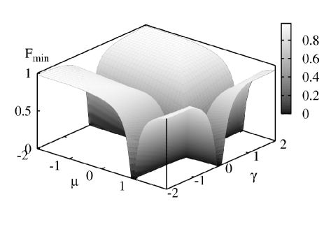
Figure 1: Fidelity $\mathcal{F}_{\text{min}}=\min[\mathcal{F}(Z,\tilde{Z}_{\delta\mu}),\mathcal{F}(Z,\tilde{Z}_{\delta\gamma})]$ (see Ref. za-co-gio ) in the $\mu$-$\gamma$ plane for $L=1001$, with $\delta\mu=\delta\gamma=0.1$. At the critical lines $\mu=1$ and $\gamma=0$ one observes an evident drop.

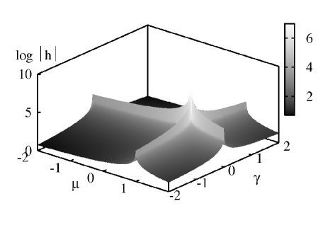
Figure 2: Decimal logarithm of the absolute value of $h(Z)$ in the $\mu$-$\gamma$ plane for $L=1001$. Note the singular behavior at $\mu=1,\gamma=0$, where the function is non-analytic. The critical lines $\mu=1$ and $\gamma=0$ emerge in a clear way.

Finally, we note that the point $\mu=1,\gamma=0$ has a peculiar singular behavior. There, all but one ($\zeta_{1}=L+\mu-1$) the eigenvalues of $Z$ vanish and the unitary $T$ is undefined (as at a first order QPT where level crossing takes place). Consequently, the angles $\Theta_{j}$ cannot be evaluated and the above formalism does not apply.

The analysis of second order QPTs can independently be done in terms of the derivatives of the GS energy $E_{0}=\mathrm{Tr}(A-\Lambda)/2=\sum_{j=1}^{L}(\Re\zeta_{j}-|\zeta_{j}|)/2$. Except on the $\mu$ axis, where $E_{0}=0$ for $\mu\geq 1$ and $E_{0}=(L-1)(\mu-1)$ for $\mu<1$, the energy scales in a superextensive way, due to the fully connected nature of the system. Indeed, while $\mathrm{Tr}A=L\mu$, for $\gamma\neq 0$ one has $\mathrm{Tr}|B|\leq\mathrm{Tr}\Lambda\leq\mathrm{Tr}|A|+\mathrm{Tr}|B|\sim\mathrm{Tr}|B|\propto{}L\ln{L}$ for $L\to\infty$. This makes it impossible to define the energy density $E_{0}/L$ in the thermodynamic limit. The density of energy derivatives can however be calculated for finite $L$ and in the TDL as well. All the second derivatives are finite and continuous for $\mu\neq 1$, $\gamma\neq 0$. For $\mu\neq 1$, $\gamma=0$ the second derivatives $\partial_{\gamma}\partial_{\mu}{}E_{0}/L$ and $\partial_{\gamma}^{2}E_{0}/L$ are analytical for $L$ finite, but in the TDL one finds the discontinuous behavior $\partial_{\gamma}\partial_{\mu}{}E_{0}(\mu\neq 1,\gamma\to 0^{\pm})/L\sim\pm{}(1/\pi)/(\mu-1)$ and the divergence $\partial_{\gamma}^{2}E_{0}(\mu\neq 1,\gamma=0)/L\propto{}S(\mu\neq 1,\gamma=0)/L\propto{}L$. It is hence reasonable to identify the critical line $\gamma=0$ with a second order QPT. Note, however, that the gap is finite at the critical point. The discontinuity and the divergence of the second derivatives of energy and fidelity at this gapful transition in the TDL is due to the divergence $\propto{}L$ of some of the single particle energies $\Lambda_{j}=|\zeta_{j}|$. This is a consequence of the unphysical long range nature of the fully coordinated model. Indeed, from Eq. (26) one has $|\zeta_{j}|\leq\sum_{k=1}^{L}|Z_{1k}|\leq\sum_{k=1}^{L}(|A_{1k}|+|B_{1k}|)$, so that $|\zeta_{j}|\propto{}L$ only if $r\propto{}L$. Another second order QPT is found at $\mu=1$, $\gamma\neq 0$, where $\partial_{\mu}^{2}E_{0}/L\propto{}\ln{L}$, while the other second derivatives are continuous. Here, however, one also has the vanishing of the lowest single particle energy, since $\Re\zeta_{j}=0$ for $j=2,\dots,L$ and $\Im\zeta_{k}\to 0$ for $L\to\infty$ with $k$ odd.

In Fig. 1 we report the GS fidelity in the $\mu$-$\gamma$ plane, by using $\mathcal{F}_{\text{min}}=\min[\mathcal{F}(Z,\tilde{Z}_{\delta\mu}),\mathcal{F}(Z,\tilde{Z}_{\delta\gamma})]$, where $\tilde{Z}_{\delta\mu}=Z(\mu+\delta\mu,\gamma)$ and $\tilde{Z}_{\delta\gamma}=Z(\mu,\gamma+\delta\gamma)$, as in Ref. za-co-gio . This corresponds to plotting the minimum of the fidelity with respect to variations along the two axes, which are related to $\partial_{\delta\mu}^{2}F_{Z}$ and $\partial_{\delta\gamma}^{2}F_{Z}$. Since the critical lines are parallel to the axes, these variations are sufficient to fully characterize the phase diagram. A detailed analysis of all the second derivatives, including also $\partial_{\delta\mu}\partial_{\delta\gamma}F_{Z}$, is instead provided by the study of $h(Z)$. The behavior of $h(Z)$ in the $\mu$-$\gamma$ plane is shown in Fig. 2 for $L=1001$. The qualitative agreement with Fig. 1 is evident.

Figure 3: Finite-size scaling (upper panel) and data collapsing (lower panel) at the critical line $\mu=1$. The upper figure shows the enhancement of the negative peak of $h$ at $\mu=1$ for $\gamma=1.5$ and $L=101,201,\dots,1001$. In the inset the curves are plotted after dividing $h$ by $L$, which allows a direct comparison with the asymptotic curve (dashed line) given by Eq. (38a). The lower figure replots the same curves of the upper figure in rescaled units. Most of them are practically indistinguishable and give rise to the thick line in the plot.

Equations (38) give the scaling of $h$ in the thermodynamic limit. It is also interesting to look at the finite-size scaling of this function, in connection with the next section about the free-ends fully coordinated system, where the simple analytical results obtained above for $L\to\infty$ are not available. The finite-size scaling for the critical line $\mu=1$ is shown in the upper panel of Fig. 3. The peak of $h$ at $\mu=1$ increases (in modulus) with $L^{2}$, as expected from Eq. (38b). Away from the minimum, the function is instead proportional to $L$, as from Eq. (38a). Consequently, the different scaling behavior makes the peak shape progressively narrower as $L$ increases. It is possible to plot the function $h$ in rescaled units in order to put in evidence these qualitative considerations. By dividing the peak depth by $L^{2}$ and rescaling the distance $\mu-1$ from the critical point by $L$ (therefore compensating the peak narrowing) one gets a curve practically independent of $L$ (data collapsing), as found in the lower panel of Fig. 3. This can be understood by looking at Eq. (38a) in the proximity of the critical line $\mu=1$, i.e., for $|\mu-1|\ll\gamma$, which is well verified for the parameters of Fig. 3. Then one finds $h\sim-L/16|\mu-1||\gamma|$, so that, for a given value of $\gamma$, the quantity $h/L^{2}$ turns out to depend only on the combination $|\mu-1|L$. Similar results were observed for the critical line $\gamma=0$.

We conclude the analysis of the cyclic fully coordinated system with a couple of additional remarks. As anticipated above, $\det{H_{F_{Z}}(0)}=0$, as one eigenvalue identically vanishes. The components of the eigenvector $\bm{v}=(v_{\mu},v_{\gamma})$ associated with this zero eigenvalue are readily found to be related by $v_{\gamma}=-(\partial^{2}_{\delta\mu}F_{Z}/\partial_{\delta\mu}\partial_{\delta\gamma}F_{Z})v_{\mu}$. Hence, since $-\partial^{2}_{\delta\mu}F_{Z}/\partial_{\delta\mu}\partial_{\delta\gamma}F_{Z}=\gamma/(\mu-1)$, the eigenvector is directed in the radial direction from the point $\mu=1,\gamma=0$. By recalling that the two eigenvectors of the symmetric matrix $H_{F_{Z}}(0)$ are mutually orthogonal, one immediately concludes that the direction of fastest GS variation is the azimuthal one with respect to this shifted origin. Finally, we comment on first order QPTs for $L$ even. In this case one has two first order critical lines, namely $\mu=1-L$ and $\mu=1$, corresponding to the vanishing of the eigenvalues $\zeta_{1}=L+\mu-1$ and $\zeta_{L/2+1}=\mu-1$ of $Z$.

IV.2 Free-ends case

In the following we discuss the free-ends fermionic graph. Some results on this system were already reported in Ref. za-co-gio . In this case the relevant matrices are not circulant and the analytic results used before are not available. In particular, it is worth stressing that the matrix $Z$ in the free-ends case is in general not normal, i.e., $[Z,Z^{T}]\neq 0$. We therefore proceed by calculating the phase diagram numerically.

Let us first recall some analytical facts za-co-gio . For $\gamma=0$ the resulting number-conserving single-particle Hamiltonian is the same as for the cyclic case. For $(\mu=0,\gamma=1)$ the matrices $Z$ and $Z^{\dagger}=Z^{T}$ become instead lower and upper triangular respectively. By explicit computation one finds $(ZZ^{T})_{ij}=4\min(L-i,L-j)$, which has the last column and row identically vanishing. Accordingly $0\in\text{Sp}\,|Z(0,1)|\;\forall\;{L}$. . We also recall that changing the sign of $\gamma$ simply corresponds to transforming $Z$ into $Z^{T}$. Hence, since $\text{Sp}(ZZ^{T})=\text{Sp}(Z^{T}Z)$, the matrix $\Lambda$ is not affected by the transformation. Then one can define $\Psi(-\gamma)=\Phi(\gamma)$ and consequently $\Phi(-\gamma)=\Psi(\gamma)$, where the matrices $\Phi$ and $\Psi$ were introduced in Sec. II. This implies that $T(-\gamma)=\Phi^{T}(-\gamma)\Psi(-\gamma)=[\Phi^{T}(\gamma)\Psi(\gamma)]^{T}=T^{T}(\gamma)$, so that the overlap behavior is symmetric with respect to the $\gamma=0$ axis.

We start from the analysis of first order QPTs. Differently from the cyclic case, the position of these transitions in the parameter space depends on $L$ in a non-trivial way, reaching however a simple configuration in the thermodynamic limit za-co-gio . First order QPTs are given by level crossings which take place when the lowest single particle energy (the gap) exactly vanishes, i.e., when $\det\Lambda=|\det{Z}|=0$. Typically, at these points one also has a discontinuous change in $\det{T}$, which jumps from $1$ to $-1$ or vice versa (corresponding to a sign change in $\det{Z}$), implying $\mathcal{F}=\sqrt{\det[(\openone+T^{-1}\tilde{T})/2]}=0$ whenever $T$ and $\tilde{T}$ are calculated at opposite sides of the transition. Strictly speaking, at the transition point where $\det{Z}=0$ the unitary $T$ is instead undefined, similarly to the azimuthal angle of polar coordinates at the origin.

In order to calculate the position of first order QPTs in the parameter space one then has to solve the equation $\det{Z}=0$. The corresponding curve in the $\mu$-$\gamma$ plane depends on $L$. Furthermore, its thermodynamic limit depends on the parity of $L$.

The results for $L$ even were already reported in Ref. za-co-gio . For $L=2$ the model is trivially solvable and one finds $\det{Z}=\mu^{2}+\gamma^{2}-1$, so that the critical line is the circle of radius one centered at the origin. For $L=4$ and $L=6$ the equation $\det{Z}=0$ is of second and third degree in $\gamma^{2}$, respectively, so that relatively simple analytical solutions are available. One gets in this way a sequence of closed curves crossing the $\mu$ axis at $\mu=1-L$ and $\mu=1$, while the $\gamma$ axis at $\gamma=\pm 1$. Numerically, in the limit $L\to\infty$ one finds the boundary $\gamma=\pm 1,\mu\leq 1$ and $|\gamma|\leq 1,\mu=1$.

Figure 4: Left panel: zeros of $\det{Z}$ in the $\mu$-$\gamma$ for $L=3$, given by $\gamma^{2}=-(\mu-1)^{2}(\mu+2)/(3\mu-2)$. Right panel: phase diagram in the $\mu$-$\gamma$ plane in the limit $L\to\infty$ for $L$ odd. Solid and dashed lines correspond to first and second order QPTs respectively.

For $L$ odd the results are different. The equation $\det{Z}=0$ for the case $L=3$ is again readily solved analytically. For any $L$, the resulting curve is now open and made of two branches. One branch starts at $\mu=1-L$, passes through $\mu=0,\gamma=\pm 1$, and diverges (as a function of $\mu$) at $\mu=\mu_{c}$, where $\mu_{c}=2/3$ for $L=3$ (see left panel of Fig. 4). The second branch trivially reduces to the point $\mu=1,\gamma=0$. The numerical analysis yields $\mu_{c}\to 1$ in the thermodynamic limit, so that the critical boundary (apart from the singular point $\mu=1,\gamma=0$) is given by $\gamma=\pm 1,\mu\leq 1$ and $|\gamma|\geq 1,\mu=1$ (see right panel of Fig. 4).

The fact that the asymptotic first order boundaries are different in the even and odd $L$ cases is at first sight surprising. In the limit $L\to\infty$, where $L+1\simeq{}L$, one would expect to find the same result in the two cases. However, the phases separated by the considered QPTs just differ by the fermion number parity. The corresponding level crossings exchange energy states with different parity (recall that the number parity is conserved by the Hamiltonian). Loosely speaking, these states, although orthogonal for any $L$, become less and less different as $L$, and hence the average number of fermions contained in the GS, increases. In conclusion, in the thermodynamic limit such first order QPTs are of little physical interest, in the sense that in practice it would be very difficult to discriminate between such phases, as it would require the capability to distinguish between $L$ and $L+1$ for $L\gg 1$. On the other hand, the different asymptotic behavior depending on the parity of $L$ is not unreasonable for a quantity which is in turn related to a parity, namely the fermion number parity.

We complete the analysis of the phase diagram by looking at the fidelity. First order QPTs appear as sudden drops of the fidelity, which falls to zero when the considered GSs are in different phases. Besides these discontinuous drops, one also observes a smooth but evident fidelity decay in the proximity of the lines $\mu=1$ and $\gamma=0$, which we identify with second order transitions za-co-gio . Hence, apart from first order QPTs, the phase diagram of the free-ends case corresponds to that of the cyclic case.

Figure 5: Finite-size scaling (upper panel) and data collapsing (lower panel) at the critical line $\mu=1$ for $\gamma>1$ and $L$ even, where (only) a second order QPT is present. The upper figure shows the enhancement of the peak of $h$ at $\mu=1$ for $\gamma=1.5$ and $L=100,200,\dots,1000$. In the insets, the law $1-\mu_{\mathrm{min}}\sim 1/L$ for the peak position (error bars correspond to numerical precision) and the function $h/L$ are shown. In the lower figure,the same curves of the upper figure are replotted in rescaled units, practically merging into an indistinguishable thick line as in the cyclic case.

It is worth discussing in some detail the critical line $\mu=1$. As explained above, for $L$ odd and $|\gamma|\geq 1$ a first order QPT is also present. For a given value $\gamma_{0}$ with $|\gamma_{0}|\in(1,\infty)$ and for finite $L$ the (first order) transition point takes place at a critical $\mu_{c}(\gamma_{0})<1$ which tends to $1$ in the thermodynamic limit (see Fig. 4). At the point $\mu_{c}(\gamma_{0}),\gamma_{0}$ the fidelity function is discontinuous and its derivatives, and hence the Hessian matrix, are not defined. However, everywhere else on the line $\gamma=\gamma_{0}$ the eigenvalue $h(Z)=\min\{\mathrm{Sp}[H_{F}(0)]\}$ can be calculated. This allows to analyze the finite-size scaling behavior of $h$ in the neighborhood of $\mu=1$ even for $|\gamma|\geq 1$. One then finds the same divergence $\propto{}L^{2}$ as for second order QPTs in the absence of first order transitions. Only, the constant of proportionality is different in the two phases (i.e., for even or odd number of fermions). For $|\gamma|<1$, instead, one only has the second order transition and $h$ is symmetric around the critical point. The position of the minimum of $h$ in the thermodynamic limit gives the second order critical line. For finite $L$ this position is given by the line $\mu=\mu_{\mathrm{min}}$, independently of $\gamma$. In the thermodynamic limit the numerical analysis gives $1-\mu_{\mathrm{min}}\sim{}1/L$, so that $\mu=1$ is the asymptotic critical line.

For $L$ even, the first order QPT interesting the $\mu=1$ transition takes place for $|\gamma|\leq 1$. Except for this difference, everything goes as in the odd $L$ case. The finite-size scaling features of $h$ around $\mu=\mu_{\mathrm{min}}$ for $L$ even and $\gamma=1.5$ are summarized in Fig. 5. It is also worth noticing that, albeit only in the TDL, the gap also vanishes in the part of the $\mu=1$ critical line where the first order QPT is absent (e.g., for $|\gamma|>1$ with $L$ even).

Another second order QPT is found along the line $\gamma=0$. Here the gap is always finite, apart from the point $\mu=1$ (see the cyclic case). Nevertheless, the finite-size scaling of $h$ puts in evidence the critical behavior. The position of the minimum of $h$ is here independent of $L$, being always given by the line $\gamma=0$.

Some insight in the nature of the latter transition can be gained by looking at the perturbative expansion of the ground state around $\gamma=0$. First of all we use a series expansion in $\gamma$ to prove analytically the $L^{2}$ divergence of $h$ in $\gamma=0$. Along the line $\gamma=0$, apart from the first order QPTs located at $\mu=1-L$ and $\mu=1$, the ground state is constant. Therefore $\partial_{\delta\mu}^{2}F_{Z}=\partial_{\delta\mu}\partial_{\delta\gamma}F_{Z}=0$ and consequently $h=\partial_{\delta\gamma}^{2}F_{Z}$. In practice, one can reduce to the one-dimensional parameter space given by $\gamma$ and use the series expansion in terms of ordinary derivatives presented in za-co-gio , $\mathcal{F}[Z(\lambda),Z(\lambda+\delta\lambda)]=1+(1/16)\mathrm{Tr}(K^{\prime}\delta\lambda)^{2}+O(\delta\lambda^{3})$, where we assumed $\det{T}=1$ so that $T=e^{K}$ and the prime denotes derivation with respect to the one-dimensional parameter $\lambda$ (not to be confused with the magnetic field strength in the XY-model). For simplicity we consider the case $\mu>1$, where $T(\gamma=0)=\openone$ and consequently $T^{\prime}(\gamma=0)=T(\gamma=0)K^{\prime}(\gamma=0)=K^{\prime}(\gamma=0)$. Lengthy but simple calculations (see Appendix B) yield

$$\mathrm{Tr}[T^{\prime}(\gamma=0)]^{2} = \frac{-1}{(\mu-1)^{2}}\frac{L(L-1)}{3[L+2(\mu-1)]^{2}}[L^{2}+$$

$$+ 2L(2\mu-3)+4(\mu-1)(3\mu-5)]\ ,$$

so that one finds $h(\gamma=0)=(1/8)\mathrm{Tr}[T^{\prime}(\gamma=0)]^{2}\sim-(1/24)[L/(\mu-1)]^{2}$ in the thermodynamic limit. Again by series expansion one has $G(\gamma)=T^{\prime}(\gamma=0)\gamma/2+O(\gamma^{2})$. The divergence of the elements of $T^{\prime}$ at $\gamma=0$ (see Appendix B) in the thermodynamic limit therefore accounts for the rapid orthogonalization rate around the critical line given by the $\mu$ axis.

V Single site entanglement

The idea of systematically using measures of quantum correlations in order to characterize QPTs has been explored in the past years for general models entanglement and in particular for the case of fermion systems vidkit ; fermionent . It was found that some of the proposed measures are able to spot, with their peculiar behavior, the undergoing QPTs; in particular, in some cases the behavior of their derivatives is universal, in the sense that they diverge with the correct critical exponents. Here we would like to complete the fidelity analysis of QPTs in the cyclic fully connected system of Subsec. IV.1 by studying of one of the simplest of such measures: the single site entanglement $\mathcal{S}_{i}=-\mathrm{Tr}(\rho_{i}\log_{2}\rho_{i})$, where $\rho_{i}=\sum_{k,h\in\{0,1\}}\rho_{h,k}\left|h\right\rangle\left\langle k\right|$ is the $2\times 2$ single site reduced density matrix PZ02 . It can be easily shown that for the system under study we have that $\rho_{0,0}=1-\rho_{1,1}=n$, where $n$ is the density. Thus the single site entanglement is given by $\mathcal{S}_{i}=-n\log n-(1-n)\log(1-n)$, where here the logarithms are taken in base $2$. It can be explicitly computed by noticing that $n=\partial(E_{0}/L)/\partial\mu$. As already described, in our case we have $E_{0}=(\mathrm{Tr}A-\mathrm{Tr}\Lambda)/2=(L\mu-\sum_{j}|\zeta_{j}|)/2$ and $n$ can be obtained by calculating the TDL of $\partial_{\mu}(\sum_{j}|\zeta_{j}|)/L=T_{ii}$. The last equality follows from the following observations: (i) since $T$ is circulant all the elements of its diagonal are equal and each of them corresponds to $T_{ii}=(\mathrm{Tr}T)/L=\sum_{j}\tau_{j}/L$, where we recall that $\tau_{j}=\zeta_{j}/|\zeta_{j}|$ are the eigenvalues of $T$; (ii) if $\zeta_{j}\in\mathrm{Sp}(Z)$ then $\zeta_{j}^{*}\in\mathrm{Sp}(Z)$ and thus $T_{ii}\in{\mathrm{I\!R}}$; (iii) the explicit formulas for $\zeta_{j}$ given in Eqs. (30)-(31) allow to write $\tau_{1}=1$, for $\mu>1-L$, which is always true in the TDL, and $\partial_{\mu}|\zeta_{j}|=(\mu-1)/|\zeta_{j}|=\Re\zeta_{j}/|\zeta_{j}|$ for $j=2,\dots,L$. We can thus write

$$T_{ii}=\frac{1}{L}+\frac{1}{L}\sum_{j=2}^{L}\Re\zeta_{j}/|\zeta_{j}|=1-2n=\frac{\partial}{\partial\mu}\frac{\mathrm{Tr}\Lambda}{L}\ .$$ (40)

The above derivation of $\mathcal{S}_{i}$ in terms of $T_{ii}$ shows the physical link between the involved quantities and in particular with the single particle eigenvalues $\zeta_{j}$. We would however like to remind that the derivation could follow other lines of reasoning based on the well known results about the evaluation of the entropy of entanglement $\mathcal{S}_{l_{1},l_{2},\dots,l_{N}}$ of a block of $N$ sites $\{l_{1},l_{2},\dots,l_{N}\}$. In fact, in Refs. vidkit ; keating04 , it is shown how to express $\mathcal{S}_{l_{1},l_{2},..,l_{N}}$ in terms of the eigenvalues $\nu_{i}$ of a matrix $S_{N}=(T_{N}T_{N}^{\dagger})^{1/2}$. There $T_{N}$ is the sub-block of order $N$, relative to the $N$ sites belonging to the block, of a matrix (called $T$ in Ref. keating04 ) equal to $\Psi^{T}\Phi$ and that is nothing but the transpose of the $T$ used in this paper. The case of the single site entanglement is then a special case of their analysis i.e., $N=1$ and, due to the circulant nature of $T$ for all $i$ one has that $S_{1}=\nu_{i}=|T_{ii}|$ and $\mathcal{S}_{l_{i}}=-[(1+\nu_{i})/2]\log[(1+\nu_{i})/2]-[(1-\nu_{i})/2]\log[(1-\nu_{i})/2]$.

We now pass to the evaluation of the TDL of $T_{ii}$ for $L$ odd. We observe that, since the single particle eigenvalues $|\zeta_{j}|$ are different for $j$ even and odd, we can split the sum in $T_{ii}$ into an even and an odd part and, since in the TDL $\sum_{k}\rightarrow(L/\pi)\int$ , we can write these sums as integrals such that:

$$T_{ii} = \frac{1}{\pi}\int_{0}^{\pi/2}\frac{(\mu-1)\mathrm{d}x}{\sqrt{(\mu-1)^{2}+\gamma^{2}\cot^{2}x}}+$$ (41)

$$+ \frac{1}{\pi}\int_{0}^{\pi/2}\frac{(\mu-1)\mathrm{d}x}{\sqrt{(\mu-1)^{2}+\gamma^{2}\tan^{2}x}}$$

The solution of these integral is different inside and outside the region $|\gamma|>|\mu-1|$. One can write

$$T_{ii}^{{}^{\prime}} = \frac{2}{\pi}\frac{\mu-1}{\sqrt{\gamma^{2}-(\mu-1)^{2}}}\ln\frac{\sqrt{\gamma^{2}-(\mu-1)^{2}}+|\gamma|}{|\mu-1|}$$

for $|\gamma|>|\mu-1|$ and

$$T_{ii}^{{}^{\prime\prime}}=\frac{2}{\pi}\frac{\mu-1}{\sqrt{(\mu-1)^{2}-\gamma^{2}}}\arcsin{\frac{\sqrt{(\mu-1)^{2}-\gamma^{2}}}{|\mu-1|}}$$ (43)

for $|\gamma|<|\mu-1|.$ $T_{ii}^{{}^{\prime}}$ can be used to study the transition $\mu\rightarrow 1$, while $T_{ii}^{{}^{\prime\prime}}$ will be used to study the transition $\gamma\rightarrow 0$. As far as $\mu\rightarrow 1$ is concerned, we first observe that $T_{ii}^{{}^{\prime}}\sim-(2/\pi)\ln|\mu-1|(\mu-1)/|\gamma|\rightarrow 0$, thus $n\rightarrow 1/2$ (half filling) and $\mathcal{S}_{i}\rightarrow 1$ is maximal On the contrary, when $\gamma\rightarrow 0$ we have that $T_{ii}^{{}^{\prime\prime}}\rightarrow\mathrm{sign}(\mu-1)$, consequently $\mathcal{S}_{i}\rightarrow 0$ and $n$ tends to zero or one, so that the ground state is factorized.

The next step is the study of the derivatives of $T_{ii}$ and $\mathcal{S}_{i}.$ One always has: $\partial_{x}\mathcal{S}_{i}=(1/2)[\log((1-|T_{ii}|)/2)-\log((1-|T_{ii}|)/2)]\partial_{x}|T_{ii}|$. We first analyze the case $x=\mu\ \ (\gamma\neq 0)$. When $\mu\rightarrow 1$ we have that $\partial_{\mu}T_{ii}^{\prime}=-2\partial_{\mu}n=\partial^{2}_{\mu}E_{0}/L\approx-\ln{|\mu-1|}/|\gamma|.$ The divergence of the density, that correctly signals the undergoing phase transition, is however not transferred to the first derivative of the single site entanglement; the latter has a maximum in $\mu=1$ and in fact we have $\partial_{\mu}\mathcal{S}_{i}\propto\log{\frac{1-|T_{ii}^{\prime}|}{1+|T_{ii}^{\prime}|}}\partial_{\mu}|T_{ii}^{\prime}|\approx(\mu-1)\log^{2}{|\mu-1|}=0$. The divergence is shifted to the derivative of second order, i.e., $\partial^{2}\mathcal{S}_{i}/\partial\mu^{2}\approx-\log^{2}{|\mu-1|}$.

We now analyze the case $x=\gamma\ \ (\mu\neq 1)$. At the transition $\gamma\to 0$ the derivative $\partial_{\gamma}T_{ii}^{\prime\prime}\to-\mbox{sign}(\gamma)2[\pi(\mu-1)]^{-1}$ is finite but, since when $\gamma\rightarrow 0$, $T_{ii}^{\prime\prime}\approx 1-2\gamma/(\pi(\mu-1))$ the derivative of the single site entanglement $\partial_{\gamma}\mathcal{S}_{i}$ diverges as $-\mbox{sign}(\gamma)\log{(|\gamma|/\pi|\mu-1|)}/|\mu-1|$.

In summary we can make the following considerations. Due to its direct link to the density $n$, the behavior of $\mathcal{S}_{i}$ in the TDL reflects the properties of the ground state: for $\gamma=0$ ($\mu\neq 1$) the state is factorized, while for $\mu=1$ ($\gamma\neq 0$) the single site quantum correlations are maximal. At the transitions the critical behavior is described by the derivatives of $\mathcal{S}_{i}$. For $\mu\rightarrow 1$ the divergence of $\partial^{2}\mathcal{S}_{i}/\partial\mu^{2}$ is again directly linked to the divergence of $\partial_{\mu}n$. In the case $\gamma\rightarrow 0$, the derivative $\partial_{\gamma}T_{ii}^{\prime\prime}$ is finite and hence it is the functional form of the chosen measure of entanglement $\mathcal{S}_{i}$ that is responsible for the divergence. Indeed $\partial_{\gamma}\mathcal{S}_{i}\propto-\log{n}+\log(1-n)$ and in this transition $n\rightarrow 0,1$ depending on $\mathrm{sign}(\mu-1)$.

VI Conclusions

In this paper we have given an extensive discussion of the relation between ground state fidelity and quantum phase transitions in quadratic Fermi systems. The presented material covers several aspects. First (i) we have provided a detailed description of the ground state calculation and a simple formula for the fidelity between ground states corresponding to different parameters. The latter expression is based on the orthogonal part $T$ of the polar decomposition of the coupling constant matrix $Z$. The fidelity behavior has then been characterized through a combination of its second derivatives, namely the minimum eigenvalue $h$ of the Hessian matrix. Subsequently (ii) we have introduced a class of models which encompass the XY fermionic Hamiltonian and are analytically solvable in the cyclic case, thereby offering a useful mean to exemplify the above concepts. In particular, we have focused on the fully connected system, whose long range nature has been shown to give rise to a peculiar gapful quantum phase transition, where $h$ exhibits critical finite-size scaling properties. Finally (iii) for the latter model in the cyclic case we have also provided an analysis of the single site entanglement, which can be extracted from the same matrix $T$ used to calculate the fidelity.

The fidelity approach to QPTs, besides being based on an intuitive understanding of the ground state dramatic change in critical regions, seems to provide further conceptual insight into these phenomena, making explicit the connections among the ground state, its energy, and the single particle spectrum. In particular, the possibility of expressing the ground state of these systems only as a function of the matrix $T$ completely clarifies its relation with the single particle energies. The latter are seen to give rise to divergences in fidelity derivatives when some of them either tend to zero or to infinite in the thermodynamic limit. The analytical solvable models presented here allow for a study of these relations in a thorough way.

We deem it appropriate to add some remarks on the possible developments of this approach. In all the models considered so far, a one to one correspondence between QPTs and fidelity drops has been observed. It would however be interesting to study the fidelity behavior in the presence of more subtle transitions, as in the case of topological QPTs, or even in crossover regions, where no discontinuous transition is present. In fact, it would be desirable to answer the question, whether fidelity drops give a reliable signature of QPTs or if they can be originated also by to other effects. In other words, could fidelity drops (or, more precisely, divergences of fidelity derivatives) provide a tool to define QPTs? In spite of the possible computational difficulty of the fidelity analysis in general systems, the added value due to the conceptual simplicity of the ideas underlying our method makes the latter, we believe, an interesting question.

Appendix A

In this appendix we prove the relationship between $\det{T}$ and the ground state number parity.

We start by proving that $\det{T}=1$ implies even parity. If $\det{T}=1$ and $-1\notin\mathrm{Sp}T$ then $T+\openone$ is invertible, $G$ exists, and the even parity follows immediately. If instead $\det{T}=1$ but $-1\in\mathrm{Sp}T$, then this negative eigenvalue must appear an even number of times in the spectrum. We note that, if $\det{T}=1$, one can write $T=e^{K}$, where $K$ is an antisymmetric real matrix. Then, a real orthogonal transformation $R$ exists such that $R^{T}KR$, and hence $R^{T}TR$, is block diagonal. For $L$ even, one has only $2\times 2$ blocks, while for $L$ odd an additional $1\times 1$ block is present, corresponding to the only unpaired eigenvalue, which is $0$ for $K$ and $1$ for $T$. Being present an even number of $-1$ eigenvalues in $\mathrm{Sp}T$, one can group them in pairs in blocks of the form $-\openone_{2}$. The idea is now to find a parity preserving canonical transformation of the $c_{i}$’s which flips the sign of the $-1$ eigenvalues of $T$. In this way one gets a matrix $T^{\prime}$ s.t. $\det{T}=1$ and $-1\notin\mathrm{Sp}T^{\prime}$, being thus possible to define $G^{\prime}=(T^{\prime}-\openone)/(T^{\prime}+\openone)$. The ground state will then have the form (7) with the transformed operators $c_{i}^{\prime}$ and the corresponding vacuum $|0^{\prime}\rangle$, so that in terms of the new parity operator $P_{N^{\prime}}=(-1)^{N^{\prime}}$, where $N^{\prime}=\sum_{j=1}^{L}{c_{j}^{\prime}}^{\dagger}{}c_{j}^{\prime}$, the ground state is even. The parity preserving nature of the canonical transformation will ensure that $P_{N^{\prime}}=P_{N}$ and the proposition be proved.

The transformation properties of the matrix $Z$ for a general real canonical transformation have been described in the first part of Sec. II. We then consider the canonical transformation $c_{j}^{\prime}=R_{jk}^{T}c_{k}$, i.e., $u=R^{T}$, $v=0$. This transformation is evidently number preserving, $N^{\prime}=\sum_{j=1}^{L}{c_{j}^{\prime}}^{\dagger}{}c_{j}^{\prime}=\sum_{j=1}^{L}c_{j}^{\dagger}{}c_{j}=N$. Furthermore one has $Z^{\prime}=R^{T}ZR=R^{T}\sqrt{ZZ^{T}}RR^{T}TR$ so that $T^{\prime}=R^{T}TR$ is block diagonal.

Without loss of generality, we now assume that the first block of $T^{\prime}$ is given by $-\openone_{2}$ and that no other $-1$ appears in the spectrum. We then use a second trivial canonical transformation defined by $u^{\prime}+v^{\prime}=\openone$ and $u^{\prime}-v^{\prime}=-\openone_{2}\oplus\openone_{L-2}$. In this way one gets $Z^{\prime\prime}=Z^{\prime}(u^{\prime}-v^{\prime})$ and $T^{\prime\prime}$ is equal to $T^{\prime}$ apart from the first two diagonal elements, whose sign is now changed. Explicitly, $u^{\prime}=\mathbb{0}_{2}\oplus\openone_{L-2}$, $v^{\prime}=\openone_{2}\oplus\mathbb{0}_{L-2}$, and it is immediate to check that $u^{\prime}$ and $v^{\prime}$ satisfy the canonical conditions (3). It is easy to see that this transformation, although not number conserving, is parity preserving. Indeed one finds $N^{\prime\prime}=N^{\prime}+2(1-n_{1}^{\prime}-n_{2}^{\prime})$, where $n_{j}^{\prime}={c_{j}^{\prime}}^{\dagger}{}c_{j}^{\prime}$, so that $P_{N^{\prime\prime}}=P_{N^{\prime}}=P_{N}$.

This proves that if $\det{T}=1$ the ground state is even. Conversely, if $\det{T}=-1$, one can find a trivial parity flipping canonical transformation which yields $T^{\prime}$ such that $\det{T^{\prime}}=1$. For example, one can choose peschel $c_{1}^{\prime}=c_{1}^{\dagger}$ and $c_{j}^{\prime}=c_{j}$ for $j=2,\dots,L$, i.e., $u=0\oplus\openone_{L-1}$ and $v=1\oplus\mathbb{0}_{L-1}$. Then $u+v=\openone$ and $u-v=-1\oplus\openone_{L-1}$, so that $T^{\prime}=T(-1\oplus\openone_{L-1})$ and hence $\det{T^{\prime}}=-\det{T}=1$. In addition, $N^{\prime}=N+1-2n_{1}$, so that the parity is flipped, $P_{N^{\prime}}=-P_{N}$. The ground state will then be of the form (7) with the transformed operators and vacuum $|0^{\prime}\rangle=c_{1}^{\dagger}|0\rangle$, being hence of even parity in the $c_{j}^{\prime}$ representation and thus odd in the original one. This completes our proof.

Appendix B

We briefly sketch the main steps of the calculation of $T^{\prime}(0)\equiv\partial_{\gamma}{}T|_{\gamma=0}$ used in Eq. (LABEL:eq:Tr[T'(0)]) of Subsec. IV.2. In the following, primed quantities imply derivation with respect to $\gamma$.

By explicitly deriving $T=\Phi^{T}\Lambda^{-1}\Phi{}Z$ with respect to $\gamma$ and using the fact that $\Lambda^{\prime}(0)=\mathbb{0}$ one finds $T^{\prime}(0)=[{\Phi^{\prime}}^{T}(0)\Phi(0),A^{-1}]A-A^{-1}B^{\prime}$, where $B^{\prime}=B/\gamma$.

To avoid the explicit calculation of $\Phi^{\prime}(0)$ one can use the relation $[A,B^{\prime}]=[{\Phi^{\prime}}^{T}(0)\Phi(0),A^{2}]$, obtained from $(ZZ^{T})^{\prime}(0)$ with the aid of $\Lambda^{\prime}(0)=\mathbb{0}$. By noting that $A^{2}=[L+2(\mu-1)]A-(L+\mu-1)(\mu-1)\openone$ [see Eq. (IV.1)] and that $[{\Phi^{\prime}}^{T}(0)\Phi(0),A^{-1}]A=-A^{-1}[{\Phi^{\prime}}^{T}(0)\Phi(0),A]$ one finds

$$T^{\prime}(0)=-A^{-1}\left(\frac{[A,B^{\prime}]}{L+2(\mu-1)}+B^{\prime}\right)\ ,$$ (44)

which, after algebraic manipulations, yields $T_{jk}^{\prime}(0)=[(k-j)/(L/2+\mu-1)-\mathrm{sign}(k-j)]/(\mu-1)$. Then, Eq. (LABEL:eq:Tr[T'(0)]) is obtained by calculating only the diagonal elements of $[T^{\prime}(0)]^{2}$, namely

$$\{[T^{\prime}(0)]^{2}\}_{jj} = \frac{1}{(\mu-1)^{2}}\left[\frac{2(\mu-1)j(j-L-1)}{(L/2+\mu-1)^{2}}+\right.$$

$$+ \left.\frac{1}{6}\frac{L(L+1)(L+6\mu-2)}{(L/2+\mu-1)^{2}}-L+1\right]\ ,$$

and finally summing to get the trace.

References

- (1) A. Osterloh, L. Amico, G. Falci, and R. Fazio, Nature 416, 608 (2002); J. Vidal, G. Palacios, and R. Mossery, Phys. Rev. A 69, 022107 (2004); J. Vidal, R. Mossery, and J. Dukelsky Phys. Rev. A 69, 054101 (2004); M.M. Wolf, G. Ortiz, F. Verstraete, and J.I. Cirac, cond-mat/0512180.
- (2) Shi-Liang Zhu, Phys. Rev. Lett. 96, 077206 (2006); A. Hamma, quant-ph/0602091; J.K. Pachos and A.C.M. Carollo, quant-ph/0602154.
- (3) S. Ryu and Y. Hatsugai, cond-mat/0601237.
- (4) H.T. Quan et al., Phys. Rev. Lett. 96, 140604 (2006); D. Rossini et al., quant-ph/0605051.
- (5) E. Farhi et al., Science 292, 472 (2001).
- (6) A. Hamma and D.A. Lidar, quant-ph/0607145.
- (7) P. Zanardi and N. Paunkovic, quant-ph/0512249, Phys. Rev. E, to be published.
- (8) P. Zanardi, M. Cozzini, and P. Giorda, quant-ph/0606130.
- (9) E. Lieb, T. Schulz, and D. Mattis, Ann. of Phys. 16, 407 (1961).
- (10) D. Rossini et al., cond-mat/0605051.
- (11) M.-C. Chung and I. Peschel, Phys. Rev. B 64, 064412 (2001); I. Peschel, J. Phys. A 36, L205 (2003).
- (12) R. Bathia, Matrix Analysis, Springer-Verlag, New York, Inc., 1997.
- (13) A. Perelemov, Generalized coherent states and their applications, Springer-Verlag , New York, Inc., 1986.
- (14) E. Barouch, B.M. McCoy, and M. Dresden, Phys. Rev. A 2, 1075 (1970); E. Barouch and B.M. McCoy, Phys. Rev. A 3, 786 (1971).
- (15) J.P. Keating and F. Mezzadri, Commun. Math. Phys. 252, 543 (2004).
- (16) H.J. Lipkin, N. Meshkov, and A.J. Glick, Nucl. Phys. 62, 188 (1965).
- (17) G. Vidal, J.I. Latorre, E. Rico, and A. Kitaev, Phys. Rev. Lett. 90, (2003) 227902.
- (18) A. Anfossi, P. Giorda, A. Montorsi, and F. Traversa, Phys. Rev. Lett. 95, 056402 (2005); A. Anfossi, C.D.E. Boschi, A. Montorsi, and F. Ortolani, Phys. Rev. B 73, 085113 (2006); S. Gu et al., Phys. Rev. Lett. 93, 086402 (2004); D. Larsson and H. Johannesson, Phys. Rev. A 73, 042320 (2006); R. Somma, G. Ortiz, H. Barnum, E. Knill, and L. Viola, Phys. Rev. A 70, 042311 (2004).
- (19) P. Zanardi, X. Wang, J. Phys. A 35, 7947 (2002); P. Zanardi, Phys. Rev. A 65, 042101 (2002).