Entanglement witnesses and a loophole problem

Abstract

We consider a possible detector-efficiency loophole in experiments that detect entanglement via the local measurement of witness operators. Here, only local properties of the detectors are known. We derive a general threshold for the detector efficiencies which guarantees that a negative expectation value of a witness is due to entanglement, rather than to erroneous detectors. This threshold depends on the local decomposition of the witness and its measured expectation value. For two-qubit witnesses we find the local operator decomposition that is optimal with respect to closing the loophole.

I Introduction

Entanglement is the central theme in quantum information processing. It allows to design faster algorithms than classically, to communicate in a secure way, or to perform protocols that have no classical analogue. Entangled states of few particles (e.g. photons, ions) can be routinely created in experiments, and their entanglement can be confirmed using state tomography, Bell inequalities or entanglement witnesses. All of these tools are well-established methods for the detection of entanglement. But can one be sure that they give a confirmative answer even when realistic, i.e. erroneous detectors are used? Here, we will introduce and study a loophole-problem for the detection of entanglement via witness operators.

Loophole-problems have been widely discussed in the context of ruling out local hidden variable (LHV) models, by measuring a violation of certain inequalities, as suggested in the seminal work of J.S. Bell in 1964 Bell . Many experiments have been carried out along that line Aspect1 , but all of them so far suffer from the locality loophole (i.e. no causal separation of the detectors) and/or the detection loophole (i.e. low detector efficiency). As a consequence of a loophole, quantum correlations are also explainable by LHV theories BellUnSpeak ; Larsson1 .

In this paper we discuss a possible detection loophole for experiments that measure entanglement witnesses. Here, the goal is not to prove the completeness of quantum mechanics (as in Bell experiments), but, assuming the correctness of quantum mechanics, to prove the existence of entanglement in a given state. One advantage of witness operators is that they require only few local measurements to detect entanglement Guehne ; global measurements are experimentally not easily accessible at present. A local projection measurement with realistic imperfect detectors (in the computational basis, for qubits and isotropic noise) can be described by the following positive operator valued measurement (POVM): $F_{0}=\xi\left|0\right>\left<0\right|,F_{1}=\xi\left|1\right>\left<1\right|,$ and $F_{2}=(1-\xi)\mathbbm{1}$, where $\xi$ is the efficiency of the detector. However, in general the global properties of the detectors are not fully characterised, e.g. there may exist correlations between POVM elements of different detectors. Provided that only local detector properties are given, what are the conditions for being nevertheless able to prove the existence of entanglement without doubt?

An entanglement witness $W$ is a Hermitian operator that fulfils $\mathrm{tr}\left(W\rho_{s}\right)\geq 0$ for all separable $n$-partite states $\rho_{s}=\sum_{i}p_{i}\bigotimes_{\nu}^{n}\big{|}\psi_{\nu}^{(i)}\big{>}\big{<}\psi_{\nu}^{(i)}\big{|}$ Werner , where the index $\nu$ numbers the subsystem, the probabilities $p_{i}$ are real and non-negative, $\sum_{i}p_{i}=1$, and $\mathrm{tr}\left(W\rho_{e}\right)<0$ for at least one entangled state $\rho_{e}$ WitnessH ; Lewenstein . Throughout this paper, we will use without loss of generality normalized witnesses, i.e. $\mathrm{tr}\left(W\right)=1$. Our goal is to ensure that a negative measured expectation value $\left<W\right>_{m}<0$ is really due to the state being entangled, rather than to imperfect detectors. The following line of arguments also holds for specialized witnesses which are constructed such that, e.g., they detect only genuine multi-partite entanglement BrussW1 or states prohibiting LHV models Hyllus .

This paper is organized as follows. After introducing the local decomposition of entanglement witnesses, we study the effect of lost events as well as additional events on the experimental expectation value of $W$. Here, we use the worst case approach to derive inequalities which need to be fulfilled to ensure entanglement of the given state. The parameters in these inequalities are the measured expectation value of the witness, the detection efficiencies, and the coefficients for the local decomposition of the witness. We show for the two-qubit case how to optimize the local operator decomposition of the witness, such that the detection efficiency which is needed to close the loophole is minimized. Some recent experiments measuring witness operators are presented, to demonstrate that the detection loophole is a problem in current experiments.

II Detection loophole for entanglement witnesses

Any witness for an $n$-partite quantum state in $d=\Pi_{\nu}^{n}d_{\nu}$ dimensions can be decomposed in a local operator basis, i.e. an $n$-fold tensor product of operators $\sigma_{\nu}^{(i)}$,

$$W=\sum_{i=0}c_{i}\bigotimes_{\nu}^{n}\sigma_{\nu}^{(i)},$$ (1)

where the coefficients $c_{i}$ are real. Each operator $\sigma_{\nu}^{(i)}$ is traceless or the identity and corresponds to the $i$th local setting for the party number $\nu$. In this expansion, we include implicitly also the local identity operators which do not need to be measured. The number of terms in eq. (1) depends on the decomposition, i.e. on the choice of operators $\sigma_{\nu}^{(i)}$. A straightforward, but not necessarily optimal choice (concerning the needed detector efficiency) are the $d_{\nu}^{2}-1$ Hermitian generators $\sigma_{\nu}$ of SU($d_{\nu}$) and the respective identity operators.

In the following, we will use a simpler notation, namely

$$W=c_{0}\mathbbm{1}+\sum_{\alpha=1}c_{\alpha}S_{\alpha},$$ (2)

where $S_{\alpha}$ stands for one term from the local expansion (1). Here, we exclude the identity $\mathbbm{1}$ (acting on the total space) from the sum over $\alpha$, because it does not have to be measured and therefore has a special role.

We will now investigate one local measurement setting described by $c_{\alpha}S_{\alpha}$, and drop the index $\alpha$ for convenience. The measured expectation value $c\left<S\right>_{m}$ is given by

$$c\left<S\right>_{m}=c\,\frac{\sum_{i}n_{i}\lambda_{i}}{N}=c\,\frac{\sum_{i}\left(\tilde{n}_{i}+\varepsilon_{+i}-\varepsilon_{-i}\right)\lambda_{i}}{\tilde{N}+\varepsilon_{+}-\varepsilon_{-}},$$ (3)

where $\lambda_{i}$ is the $i$th eigenvalue of $S$, the number of measured events for the $i$th outcome is denoted as $n_{i}$, and $N$ is the total number of measured events for that setting. In the second part of eq. (3) we expressed this expectation value as a sum of the ideal number of events, denoted as $\tilde{n}_{i}$ (i.e. for perfect detectors), the additional events $\varepsilon_{+i}$ (e.g. dark counts) and the lost events $\varepsilon_{-i}$ for the $i$th outcome. The total ideal number of events for such a setting is denoted as $\tilde{N}$, and the total number of additional/lost events as $\varepsilon_{\pm}$. We have $\tilde{N}=\sum_{i}\tilde{n}_{i}$ and $\varepsilon_{\pm}=\sum_{i}\varepsilon_{\pm i}$.

The experimental data usually gives no information about the number of errors $\varepsilon_{\pm i}$ for a specific measurement outcome $i$. Only the detection imperfections are known, namely the detection efficiency (“lost events efficiency”):

$$\eta_{-}=\frac{\tilde{N}-\varepsilon_{-}}{\tilde{N}}$$ (4)

and the “additional events efficiency”:

$$\eta_{+}=\frac{\tilde{N}}{\tilde{N}+\varepsilon_{+}},$$ (5)

where $0\leq\eta_{\pm}\leq 1$ holds. Here, $\eta_{\pm}$ denotes the global detection efficiency for a given measurement setting. In the following, we assume that $\eta_{\pm}$ is the same for all settings. (Other cases can be included by indexing $\eta_{\pm}$ with $\alpha$.)

Usually, one makes the fair-sampling assumption about the statistical distribution of the unknown errors $\varepsilon_{\pm i}$, i.e. one assumes the same statistical distribution for detected and lost events; the additional events are assumed to have a flat distribution. Here, we will give up this assumption and will consider the worst case, where both lost and additional events contribute such that the expectation value of the witness is shifted towards negative values. We point out that in order to reach this worst case scenario, it is already sufficient that the global POVM elements exhibit certain classical correlations (while being compatible with the local measurement operators) tobepu .

The worst case is equivalent to finding the lowest possible $c\left<S\right>_{m}$, which is achieved by minimizing the contribution of the additional events, and maximizing the contribution of the lost events in eq. (3). This minimization/maximization can be easily shown to have the form $\min_{\varepsilon_{+i}}c\sum_{i}\varepsilon_{+i}\lambda_{i}=\varepsilon_{+}\Omega_{+}$ and $\max_{\varepsilon_{-i}}c\sum_{i}\varepsilon_{-i}\lambda_{i}=\varepsilon_{-}\Omega_{-}$, with

$$\Omega_{\pm}=c\left(\Theta(\pm c)\lambda_{\mathrm{min}}+\Theta(\mp c)\lambda_{\mathrm{max}}\right),$$ (6)

where $\Theta(x)$ denotes the Heaviside function, and $\lambda_{\mathrm{min/max}}$ is the minimal/maximal eigenvalue of $S$.

Inserting this into eq. (3), one finds the following worst case estimate for the measured expectation value $c\left<S\right>_{m}$:

$$c\left<S\right>_{m}=\kappa\left(c\left<S\right>_{t}-\Omega_{+}(1-\frac{1}{\eta_{+}})-\Omega_{-}\left(1-\eta_{-}\right)\right),$$ (7)

where $\kappa:=\tilde{N}\left(\tilde{N}+\varepsilon_{+}-\varepsilon_{-}\right)^{-1}=\left(\frac{1}{\eta_{+}}+\eta_{-}-1\right)^{-1}$. Here, we have introduced the notation $c\left<S\right>_{t}$ for the true expectation value (without any errors).

Using $\left<W\right>_{m/t}=c_{0}+\sum_{\alpha}c_{\alpha}\left<S_{\alpha}\right>_{m/t}$ and eq. (7), with isotropic detection efficiencies, we can express the measured witness expectation value $\left<W\right>_{m}$ as a function of the true one $\left<W\right>_{t}$, for the worst case. To close the loophole it is necessary to ensure that $\left<W\right>_{t}<0$. This leads to a condition for the maximal $\left<W\right>_{m}$ that depends on the decomposition of $W$ and the efficiencies $\eta_{\pm}$:

$$\left<W\right>_{m} < c_{0}(1-\kappa)-$$ (8)

$$\kappa\sum_{\alpha}\left(\Omega_{\alpha+}\left(1-\frac{1}{\eta_{+}}\right)+\Omega_{\alpha-}\left(1-\eta_{-}\right)\right)\!\!,\>{}$$

where we have re-introduced the summation index $\alpha$.

¿From now on we want to focus on the case where the subsystems are two-dimensional, i.e. qubits. For qubits the measurement operators $S_{\alpha}$ are chosen to be tensor products of Pauli operators with eigenvalues $\lambda=\pm 1$. This simplifies $\Omega_{\pm}$ to $\Omega_{\alpha\pm}=\mp\left|c_{\alpha}\right|$, and eq. (8) reads for qubits

$$\left<W\right>_{m}<c_{0}-\frac{c_{0}+\sum_{\alpha}\left|c_{\alpha}\right|\left(\frac{1}{\eta_{+}}-\eta_{-}\right)}{\eta_{-}+\frac{1}{\eta_{+}}-1}.$$ (9)

In Fig. 1 a contour plot of this function is shown: Given a certain measured expectation value $\left<W\right>_{m}$, the corresponding efficiencies $\eta_{\pm}$ ensure that the state is indeed entangled. This plot assumes $c_{0}+\sum_{\alpha}\left|c_{\alpha}\right|=1$, and can be easily redrawn for other decompositions.

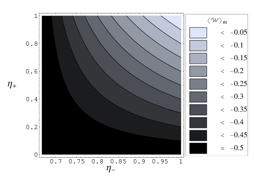
Figure 1: The contours correspond to the maximal $\left<W\right>_{m}$ of a multipartite qubit witness which still ensures entanglement, where a decomposition with $c_{0}+\sum_{\alpha}\left|c_{\alpha}\right|=1$ was assumed, which is e.g. achieved for an optimal two qubit Bell state witness $W_{\phi^{+}}$ (see text).

¿From eq. (9) it is obvious that an optimal decomposition of such a witness with respect to the needed efficiencies $\eta_{\pm}$ is achieved by minimizing $\sum_{\alpha}\left|c_{\alpha}\right|$. For the case of two-qubit witnesses a constructive optimization can be achieved, when arbitrary local Stern-Gerlach measurements (described by Pauli operators or rotations thereof) and the identity are allowed. We start with a two-qubit witness in its Pauli operator decomposition, i.e.

$$W = c_{00}\mathbbm{1}\otimes\mathbbm{1}+\mathbbm{1}\otimes\left(\sum_{j=1}^{3}c_{0j}\sigma_{j}\right)+$$ (10)

$$\left(\sum_{i=1}^{3}c_{i0}\sigma_{i}\right)\otimes\mathbbm{1}+\sum_{i,j=1}^{3}c_{ij}\sigma_{i}\otimes\sigma_{j},$$

where $\sigma_{1/2/3}=\sigma_{x/y/z}$ and $c_{ij}\in\mathbbm{R}$. The normalization condition $\mathrm{tr}\!\left(W\right)=1$ leads to $c_{00}=\frac{1}{4}$. The three remaining terms in eq. (10) can be optimized separately (note the special role of the identity).

Let us first consider the term $W_{3}=\sum_{i,j=1}^{3}c_{ij}\sigma_{i}\otimes\sigma_{j}$. This expression is optimized by doing a singular value decomposition of the coefficient matrix $(C)_{ij}=c_{ij}$, i.e. $UCV^{\dagger}=S$, where $S$ is the diagonal matrix that contains the singular values $s_{i}$. The matrices $U$ and $V$ are orthogonal and have entries $u_{ij}$ and $v_{ij}$. The new orthogonal basis is simply constructed by using the orthonormal rows of $U$ and $V$, i.e. $\tilde{\sigma}_{Ai}=\sum_{j}u_{ij}\sigma_{j}$ and $\tilde{\sigma}_{Bi}=\sum_{j}v_{ij}\sigma_{j}$, such that we get the Schmidt operator decomposition

$$W_{3} = \sum_{i=1}^{3}s_{i}\tilde{\sigma}_{Ai}\otimes\tilde{\sigma}_{Bi},$$ (11)

with $\frac{1}{2}\mathrm{tr}\!\left(\tilde{\sigma}_{Ai}\tilde{\sigma}_{Aj}\right)=\delta_{ij}$ and the same orthogonality relation for party $B$.

The optimality of this biorthogonal decomposition with respect to the detector efficiencies is shown as follows: Consider the most general decomposition $W_{3}=\sum_{j}^{M}b_{j}\sigma^{\prime}_{Aj}\otimes\sigma^{\prime}_{Bj}$, where $\sigma^{\prime}_{A/Bj}$ are arbitrary (not necessarily orthogonal) rotated Pauli operators and without loss of generality $b_{j}>0$ (we can include a minus sign in one of the operators). Here, the number of terms $M$ is finite and an operator may appear more than once.

We can express this decomposition in terms of our orthogonal basis $\tilde{\sigma}_{A/Bi}$,

$$W_{3}=\sum_{j}^{M}b_{j}\sigma^{\prime}_{Aj}\otimes\sigma^{\prime}_{Bj}=\sum_{j,k,l}b_{j}\alpha_{k}^{(j)}\beta_{l}^{(j)}\tilde{\sigma}_{Ak}\otimes\tilde{\sigma}_{Bl},$$ (12)

with $\sum_{k}\left(\alpha_{k}^{(j)}\right)^{2}=\sum_{k}\left(\beta_{k}^{(j)}\right)^{2}=1$ for all $j$. The right hand sides of eq. (11) and eq. (12) are equal. We multiply these two expressions by $\sum_{m}\tilde{\sigma}_{Am}\otimes\tilde{\sigma}_{Bm}$ and take the trace on both sides. This leads to

$$\sum_{i,m}s_{i}\mathrm{tr}\!\left(\left[\tilde{\sigma}_{Ai}\otimes\tilde{\sigma}_{Bi}\right]\left[\tilde{\sigma}_{Am}\otimes\tilde{\sigma}_{Bm}\right]\right)=$$

$$\sum_{j,k,l,m}b_{j}\alpha_{k}^{(j)}\beta_{l}^{(j)}\mathrm{tr}\!\left(\left[\tilde{\sigma}_{Ak}\otimes\tilde{\sigma}_{Bl}\right]\left[\tilde{\sigma}_{Am}\otimes\tilde{\sigma}_{Bm}\right]\right).$$ (13)

Orthogonality of the basis is used to get

$$\sum_{i}s_{i} = \sum_{j,m}b_{j}\alpha_{m}^{(j)}\beta_{m}^{(j)}\leq\sum_{j}b_{j},$$ (14)

where we used the fact that the scalar product between two normalized vectors ($\vec{\alpha}^{\,(j)}$ and $\vec{\beta}^{\,(j)}$) is less or equal to one. This proves the optimality of the decomposition of $W_{3}$ given in eq. (11).

The third term in eq. (10) – and, analogously, the second one – can be written as

$$W_{2}=\tilde{c}_{10}\left(\sum_{i=1}^{3}\alpha_{i}\sigma_{i}\right)\otimes\mathbbm{1}=\tilde{c}_{10}\tilde{\sigma}_{10}\otimes\mathbbm{1},$$ (15)

where $\tilde{\sigma}_{10}$ is a rotated Pauli operator, $\sum_{i}\alpha_{i}^{2}=1$ and $\tilde{c}_{10}>0$. Following similar arguments as before, it is easy to verify that $\tilde{c}_{10}$ is optimal.

The situation for higher dimensions is different: It is unfortunately not straightforward to generalize the above optimization to higher-dimensional witnesses, because we extensively used the fact that a linear combination of Pauli operators is again a scaled rotated Pauli operator. Also, for multi-partite witnesses the Schmidt decomposition eq. (11) does not always exist, such that our optimization method is not applicable for these cases.

In many experimental situations, e.g. when optical detectors are used, only the “lost event efficiency” is an important issue and the “additional event efficiency” is approximately $\eta_{+}\approx 1$ Barbieri ; Bourennane . This situation further simplifies eq. (8), and the minimal detector efficiency that allows to close the loophole has a simple relation with the measured expectation value and the decomposition of the witness, namely

$$\eta_{-}>\left(1-\frac{\left<W\right>_{m}}{c_{0}+\sum_{\alpha}\left|c_{\alpha}\right|}\right)^{-1}.$$ (16)

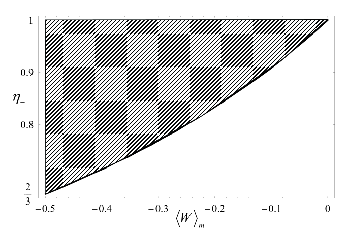
Figure 2: The detector efficiency loophole is closed (assuming $\eta_{+}=1$) if the detector efficiency ($\eta_{-}$) is in the hatched area for a given measured expectation value $\left<W\right>_{m}$. Here, a decomposition with $c_{0}+\sum_{\alpha}\left|c_{\alpha}\right|=1$ is assumed.

This function is shown in fig. (2), where the hatched area corresponds to values for which the inequality is fulfilled, again assuming $c_{0}+\sum_{\alpha}\left|c_{\alpha}\right|=1$. For two qubits the detection loophole for witnesses can already be closed with a detection efficiency $\eta_{-}>\frac{2}{3}$. This bound is sufficient e.g. for the optimal two-qubit witness of a Bell state and a measured expectation value of $\left<W\right>_{m}=-\frac{1}{2}$. We conjecture that for $\eta_{-}<\frac{2}{3}$ the loophole cannot be closed for any witness.

III Experimental examples and summary

We now want to discuss some prominent experimental examples in this context. In ion trap experiments the detection efficiencies are close to one ($\sim 99.8\%$) ZollerIonTrap and the detection loophole is usually not an issue. Exceptions are many-party-witnesses with expectation values close to zero, like the genuine 8-qubit multipartite entanglement witness experiment of Häffner et al. Haeffner .

Single photon experiments on the other hand are more problematic. Using eq. (16) we give some explicit experimental examples for the needed detection efficiencies to close the witness loophole: M. Barbieri et al. Barbieri implemented the optimal two-qubit entanglement witness to detect a Bell state, where they achieved an expectation value of $-0.493\pm 0.008$. In this case the detection efficiency needs to be $\eta_{-}>0.67$. In recent experiments also multipartite entanglement witnesses were implemented Bourennane . In this work the three-qubit GHZ entanglement witness is loophole-free with a detection efficiency of $\eta_{-}>0.91$, and the four-partite case needs $\eta_{-}>0.94$. Single photon detector efficiencies for wavelengths of 700-800 nm are typically around 70% DetectEffKwiat , such that the global detection efficiency for two qubits is circa 50 % , and even lower for more than two subsystems. The detection efficiencies for multipartite witness experiments with photons are thus considerably below the needed thresholds. This is a similar situation as for the detection loophole in Bell inequalities Larsson1 . However, there is a good chance for loophole-free witness experiments with two qubits, when slightly more efficient detectors are available.

In summary, we discussed the detection loophole problem for experiments measuring witness operators. Assuming the worst case (that may occur due to unknown global properties of the detectors) we derived certain inequalities to close such loopholes. These inequalities are generally valid for any type of witness operator and depend on the measured expectation value of the witness, its local operator decomposition and the detector efficiencies. ¿From there, detector efficiency thresholds to close the loophole are easily calculated. The local decomposition of the witness can be optimized such that the needed detection efficiencies are minimized. We explicitly presented a constructive optimization for two-qubit witnesses. For multi-qubit witnesses the optimal decomposition is achieved by minimizing the sum of the absolute values of the expansion coefficients. In the case of higher-dimensional witnesses the optimization is not straightforward any more, because it then also depends on the type of operator basis. Let us mention that an analogous study can be performed, if the witness is decomposed into local projectors Guehne2 ; this will be published elsewhere. For qubit witnesses we further considered the common experimental situation, where additional counts can be neglected. Current witness experiments with polarized photons do not close the detection loophole, because of the low single photon detector efficiencies. – Further research directions and open problems include the optimal local decomposition for higher-dimensional witnesses, and the case of erroneous detector orientations.

We acknowledge discussions with Harald Weinfurter. This work was supported in part by the European Commission (Integrated Projects SCALA and SECOQC).

References

- (1) J. S. Bell, Physics (Long Island City, NY) 1, 195 (1964)
- (2) A. Aspect, P. Grangier, and G. Roger, Phys. Rev. Lett. 47, 460 (1981); A. Aspect, P. Grangier, and G. Roger, Phys. Rev. Lett. 49, 91 (1982); A. Aspect, J. Dalibard, and G. Roger, Phys. Rev. Lett. 49, 1804 (1982); G. Weihs, T. Jennewein, C. Simon, H. Weinfurter, and A. Zeilinger, Phys. Rev. Lett. 81, 5039 (1998); M.A. Rowe et al., Nature 409, 791 (2001).
- (3) J. S. Bell, Speakable And Unspeakable In Quantum Mechanics (Cambridge University Press), EPR-Experiments, (1987); T. K. Lo and A. Shimony, Phys. Rev. A 23, 3003 (1981); A. Garg and N. D. Mermin, Phys. Rev. D 35, 3831 (1987).
- (4) J.-Å. Larsson, Phys. Rev. A 57, 3304 (1998).
- (5) O. Gühne, P. Hyllus, D. Bruß, A. Ekert, M. Lewenstein, C. Macchiavello, and A. Sanpera, Phys. Rev. A 66, 62305 (2002).
- (6) R.F. Werner, Phys. Rev. A, 40, 4277 (1989).
- (7) M. Horodecki et al., Phys. Lett. A, 223, 1 (1996).
- (8) M. Lewenstein, B. Kraus, J. I. Cirac, and P. Horodecki, Phys. Rev. A 62, 052310 (2000).
- (9) D. Bruß et al., J. Mod. Opt., 49, 1399 (2002).
- (10) P. Hyllus, O. Gühne, D. Bruß, and M. Lewenstein, Phys. Rev. A 72, 12321 (2005).
- (11) H. Kampermann et al., to be publ.
- (12) M. Barbieri et al., Phys. Rev. Lett., 91, 227901 (2003).
- (13) M. Bourennane et al., Phys. Rev. Lett., 92, 87902 (2004).
- (14) J.I. Cirac, P. Zoller, Phys. Rev. Lett., 74, 4091 (1995).
- (15) H. Häffner et al., Nature, 438, 643 (2005).
- (16) P. G. Kwiat, A.M. Steinberg, R.Y. Chiao, P.H. Eberhard, M.D. Petroff, Phys. Rev. A, 48, R867 (1993).
- (17) O. Gühne et al., Phys. Rev. A, 66, 062305 (2002).