Time Optimal Unitary Operations

Abstract

Extending our previous work on time optimal quantum state evolution [A. Carlini, A. Hosoya, T. Koike and Y. Okudaira, Phys. Rev. Lett. 96, 060503 (2006)], we formulate a variational principle for finding the time optimal realization of a target unitary operation, when the available Hamiltonians are subject to certain constraints dictated either by experimental or by theoretical conditions. Since the time optimal unitary evolutions do not depend on the input quantum state this is of more direct relevance to quantum computation. We explicitly illustrate our method by considering the case of a two-qubit system self-interacting via an anisotropic Heisenberg Hamiltonian and by deriving the time optimal unitary evolution for three examples of target quantum gates, namely the swap of qubits, the quantum Fourier transform and the entangler gate. We also briefly discuss the case in which certain unitary operations take negligible time.

I Introduction

Time optimal quantum computation is attracting a growing attention khaneja ; zhang ; schulte ; boscain besides the more conventional concept of optimality in terms of gate complexity, i.e. the number of elementary gates used in a quantum circuit chuangnielsen . The minimization of physical time to achieve a given unitary transformation is relevant for the design of fast elementary gates. It also provides a physical ground to describe the complexity of quantum algorithms, whereas gate complexity should be regarded as a more abstract concept in which physics is implicit. Works relevant to the former subject can be found, e.g., in khaneja and zhang , which discuss the time optimal generation of unitary operations for a small number of qubits using a Cartan decomposition scheme and assuming that one-qubit operations can be performed arbitrarily fast. An adiabatic solution to the optimal control problem in holonomic quantum computation was given in tanimura , while Schulte-Herbrüggen et al. schulte numerically obtained improved upper bounds on the time complexity of certain quantum gates. The present authors CarHosKoiOku06PRL discussed the quantum brachistochrone for state evolution, i.e. the problem of finding the time optimal evolution and the optimal Hamiltonian of a quantum system for given initial and final states. Nielsen et al. nielsen1 proposed a criterion for optimal quantum computation in terms of a certain geometry in Hamiltonian space, and showed in nielsen2 that the quantum gate complexity is related to optimal control cost problems. Khaneja et al. khanejanew suggested a geometrical method for the efficient synthesis of the controlled-not gate between two qubits with a special Hamiltonian.

In the standard quantum computation paradigm a whole algorithm may be reduced to a sequence of unitary transformations between intermediate states and a final measurement to read the result. In this paper we address the time optimality of each unitary transformation, i.e., each subroutine. An example is the discrete Fourier transform in Shor’s algorithm for factorization.

In our previous work CarHosKoiOku06PRL , the quantum brachistochrone was formulated as an action principle for the quantum state in the complex projective space endowed with the Fubini-Study metric, and the Hamiltonian subject to certain constraints. We obtained the time optimal state evolution and the optimal Hamiltonian by solving the Euler-Lagrange equations. In the present work we extend the methods used in CarHosKoiOku06PRL and we describe the general framework for finding the time optimal realization of a given unitary operation. Roughly speaking, we replace the projective space representing quantum state vectors with the space of unitary operators. While the optimality in the previous work depends on the initial state, it does not in the present case so that it is more directly relevant to subroutines in quantum computation, where the input may be unknown. This work should be useful not only for designing the efficient quantum algorithms and devices but also for deepening our insight into the true origin of the power of quantum computation.

The paper is organized as follows. In Section II we introduce the problem by defining an action principle for the time optimal realization of unitary operations, under the condition of a Schrödinger evolution and of the existence of a set of constraints for the available Hamiltonians, and we derive the fundamental equations of motion. We discuss a typical class of the problem in Section III. In Section IV we explicitly show how our formalism works via the example of a two-qubit system, which self-interacts by an anisotropic Heisenberg Hamiltonian depending on several control parameters. We derive the time optimal controls and the optimal time duration required to generate a swap gate, a ‘qft’ gate and an entangler gate. A system in which certain operations take negligible time is discussed briefly in Section V. Finally, Section VI is devoted to the summary and discussion of our results.

II A variational principle

Let us consider the problem of performing a given unitary operation or a quantum subroutine in the shortest time by controlling a certain physical system. Mathematically this is a time optimality problem of achieving a unitary operator $U_{f}\in\operatorname{\it U}(N)$ (modulo overall phases) by controlling the Hamiltonian $H(t)$ and evolving a unitary operator $U(t)$, where $H(t)$ and $U(t)$ obey to the Schrödinger equation. Note that overall phases are physically irrelevant for quantum evolutions. One immediately observes that there must be some constraints for $H(t)$, because otherwise one would be able to realize $U_{f}$ in an arbitrarily short time simply by rescaling the Hamiltonian CarHosKoiOku06PRL . Thus at least the ‘magnitude’ of the Hamiltonian must be bounded. Physically this corresponds to the fact that one can afford only a finite energy in the experiment. Besides this normalization constraint, the available Hamiltonians may be subject also to other constraints, which can represent either experimental requirements (e.g., the specifications of the apparatus in use) or theoretical conditions (e.g., allowing no operations involving three or more qubits).

We then define the following action for the dynamical variables $U(t)$ and $H(t)$,

$$S(U,H,\Lambda,\lambda_{j}):= \int dt\left[L_{T}+L_{S}+L_{C}\right]$$ (1)

with

$$L_{T}:=\sqrt{\frac{\langle\tfrac{dU}{dt},(1-P_{U})\left(\tfrac{dU}{dt}\right)\rangle}{\langle HU,(1-P_{U})(HU)\rangle}},$$ (2)

$$L_{S}:=\langle\Lambda,i\tfrac{dU}{dt}U^{\dagger}-H\rangle,$$ (3)

$$L_{C}:=\sum_{j}{\lambda_{j}}f^{j}(H),$$ (4)

where we have introduced the Hilbert-Schmidt norm ${\left\langle A,B\right\rangle}:=\operatorname{Tr}A^{\dagger}B$ and the projection $P_{U}(A):=\tfrac{1}{N}\operatorname{Tr}(AU^{\dagger})U$. The Hermitian operator $\Lambda(t)$ and the scalars $\lambda_{j}(t)$ are Lagrange multipliers. The action term $\int L_{T}dt$ gives the time duration to be optimized and corresponds to the action $\int[ds/v]$, where $v$ is the velocity of the particle, in the classical brachistochrone. The metric

$$ds_{\text{\tiny$U$}}^{2}=\langle dU,(1-P_{U})(dU)\rangle$$ (5)

is analogous to the Fubini-Study metric $ds_{\text{\tiny$FS$}}^{2}=\langle{d\psi}|(1-|{\psi}\rangle\!\langle{\psi}|)|{d\psi}\rangle$ for the quantum state $|{\psi}\rangle$ and is invariant under left and right global $U(N)$ multiplications.

The variation of $L_{S}$ by $\Lambda$ gives the Schrödinger equation

$$i\frac{dU}{dt}=HU,\quad\text{or}\quad U(t)={\mathcal{T}}e^{-i\int^{t}_{0}Hdt},$$ (6)

where $\mathcal{T}$ is the time ordered product. This is similar to the case of the quantum brachistochrone for quantum states CarHosKoiOku06PRL . On the other hand, the variation of $L_{C}$ by $\lambda_{j}$ leads to the constraints for $H$,

$$f_{j}(H)=0.$$ (7)

If we assume that the constraint functions $f_{j}(H)$ depend only on the traceless part of $H$, i.e. $\widetilde{H}:=(1-P_{1})(H)=H-(\operatorname{Tr}H)1/N$, thanks to the projection $P_{U}$ in 2 the action $S$ is invariant under the $U(1)$ gauge transformation

$$U\mapsto e^{i\theta}U,~{}H\mapsto H-\tfrac{d\theta}{dt},~{}\Lambda\mapsto\Lambda,~{}\lambda_{j}\mapsto\lambda_{j},$$ (8)

where $\theta$ is a real function. In the following we will consider the time optimal evolution of operators belonging to the group $\operatorname{\it U}(N)/\operatorname{\it U}(1)\simeq\operatorname{\it SU}(N)$. This is natural because overall phases are irrelevant in quantum mechanics. To present our method in its simplest form, we have restricted ourselves to the case where the gauge degree of freedom is $U(1)$. However, when there are quantum operations whose time duration is so short that it can be neglected, we will have a larger gauge group $K$. Such a case is discussed briefly in Section V.

We incidentally note here that, when the Hamiltonian is time independent, the unitary operator actually evolves along a geodesic with respect to the metric ${ds}_{\text{\tiny$U$}}^{2}$. This can be easily seen from 6, which implies

$$\tfrac{d}{dt}\left[(1-P_{1})\left(\tfrac{dU}{dt}U^{\dagger}\right)\right]=0,$$ (9)

the same equation as derived from the variation by $U$ of the arclength $\int ds_{\text{\tiny$U$}}$.

Let us now derive the other equations of motion. Before taking variations of the action, it is convenient to rewrite $L_{T}$ as

$$L_{T}=\sqrt{\frac{\langle\tfrac{dU}{dt}U^{\dagger},(1-P_{1})(\tfrac{dU}{dt}U^{\dagger})\rangle}{\langle H,(1-P_{1})(H)\rangle}},$$ (10)

where we have used the relation $P_{U}(A)=P_{1}(AU^{\dagger})U$. Then the variation of $S$ by $H$ gives

$$-L_{T}\cdot\frac{(1-P_{1})(H)}{\langle H,(1-P_{1})(H)\rangle}-\Lambda+F=0,$$ (11)

where we have introduced the operator

$$F:={\partial{L_{C}}\over\partial{H}},$$ (12)

which plays an important role in the following. Using 6, which implies $L_{T}=1$, and recalling that $(1-P_{1})(H)=\widetilde{H}$, one can rewrite 11 as

$$\Lambda=F-\frac{\widetilde{H}}{\operatorname{Tr}\widetilde{H}^{2}}.$$ (13)

Let us now take the variation of $S$ by $U$. We first note that

$$\operatorname{Tr}A\delta{\left(\frac{dU}{dt}U^{\dagger}\right)}=\operatorname{Tr}D[A]U\delta U^{\dagger}$$ (14)

for any $A$ up to a total time derivative, where $D[A]:={{d{A}}\over{d{t}}}+[A,{{d{U}}\over{d{t}}}U^{\dagger}]$. The equation above holds because $\delta U^{\dagger}=-U^{\dagger}\delta UU^{\dagger}$ and $\tfrac{dU^{\dagger}}{dt}=-U^{\dagger}\tfrac{dU}{dt}U^{\dagger}$. Using 10 and 14, one can easily calculate $\delta S/\delta U=0$ to obtain

$$D\left[{L_{T}}\cdot\frac{(1-P_{1})(\tfrac{dU}{dt}U^{\dagger})}{\langle\tfrac{dU}{dt}U^{\dagger},(1-P_{1})(\tfrac{dU}{dt}U^{\dagger})\rangle}+i\Lambda\right]=0.$$ (15)

When the Schrödinger equation 6 and 13 for $\Lambda$ hold, one finds that the argument of $D$ above is simply $iF$. We thus have $D[F]=0$. Rewriting this, we obtain the quantum brachistochrone equation

$$i\frac{dF}{dt}=[H,F],\quad\text{or}\quad F(t)=U(t)F(0)U^{\dagger}(t).$$ (16)

This, together with the Schrödinger equation 6 and the constraints 7, is our fundamental equation kosloff . The quantum brachistochrone equation 16 seems universal, as it holds also in the case of time optimal evolution of pure CarHosKoiOku06PRL and mixed next quantum states oldF . In particular, equation 16 implies a simple conservation law,

$$\operatorname{Tr}F^{m}=\text{const.},\quad m=1,2,....$$ (17)

In order to solve the quantum brachistochrone equation 16, one should first eliminate the gauge freedom 8. The most natural gauge choice is to take $H$ to be traceless, i.e.,

$$H=\widetilde{H}.$$ (18)

This corresponds to choosing the unitary operator $U$ to be an element of $\operatorname{\it SU}(N)$. Then, for a given operation $U_{f}$, the procedure to find the optimal Hamiltonian $H$ and the optimal time duration $T$ as follows:

(i) specify the functions $f_{j}(H)$ which constrain the range of available Hamiltonians;

(ii) write down the quantum brachistochrone equation 16;

(iii) solve 16 together with the constraints 7 to obtain $H(t)$;

(iv) integrate the Schrödinger equation 6 with $U(0)=1$ to get $U(t)$;

(v) fix the constants in $H(t)$ by imposing the condition that $U(T)$ equals $U_{f}$ modulo a global $U(1)$, i.e.,

$$U(T)=e^{i\chi}~{}U_{f},$$ (19)

where $\chi$ is some real number.

In essence, we have reduced the problem of finding the time optimal unitary evolution, for Hamiltonians subject to certain constraints, to a set of first-order ordinary differential equations, which we call the quantum brachistochrone equation. Such an equation can always be solved in the general $\operatorname{\it U}(N)$ case, e.g. numerically.

III Typical class of constraints

Let us now discuss a typical and important class of constraints. We assume that the normalization condition for $H$, i.e., the finite energy condition, can be written in the form

$$f(H):=\tfrac{1}{2}(\operatorname{Tr}\widetilde{H}^{2}-N\omega^{2})=0,$$ (20)

where $\omega$ is a constant. Then the constraint part of the Lagrangian can be rewritten as

$$L_{C}=\lambda f(H)+L_{C}^{\prime},$$ (21)

where $\lambda$ is a Lagrange multiplier and $L_{C}^{\prime}$ is the sum of the other constraints. Therefore, from 12, 20 and 21 we obtain

$$F=\lambda\widetilde{H}+F^{\prime},$$ (22)

where $F^{\prime}:={\partial{L_{C}^{\prime}}\over\partial{H}}$. Multiplying 22 by $U$ from the right, using the quantum brachistochrone equation 16, the Schrödinger equation 6 and 18, we have $i\lambda\dot{U}+F^{\prime}U=UF(0)$. By formal integration, we get

$$U={\left[{\cal T}\exp{\left(i\int_{0}^{t}\frac{F^{\prime}dt}{\lambda}\right)}\right]}\exp{\left(-iF(0)\int_{0}^{t}\frac{dt}{\lambda}\right)}.$$ (23)

The system becomes particularly simple if the constraints for $H$ are, except for the finite energy condition 20, linear and homogeneous in $\widetilde{H}$, namely, if

$$L_{C}^{\prime}=\operatorname{Tr}\widetilde{H}F^{\prime},$$ (24)

where $F^{\prime}=\sum_{j}\lambda_{j}g_{j}$ with $g_{j}\in\operatorname{\mathfrak{s}\mathfrak{u}}(N)$, so that we have:

$$\operatorname{Tr}g_{j}\widetilde{H}=0.$$ (25)

Many problems in quantum computation or quantum control, including the example in the following section, fall into this subclass. Note that with the assumption 24 $F^{\prime}$ does not depend on the Hamiltonian $H$ explicitly.

We can easily show that $\lambda$ in 22 is a constant. Choosing the gauge 18, we have

$$0=\operatorname{Tr}\widetilde{H}{{d{F}}\over{d{t}}}=N\omega^{2}{{d{\lambda}}\over{d{t}}},$$ (26)

where the first equality follows from 16 and the second one from the constraints 20 and 25. Thus $\lambda$ is a constant, which can be chosen equal to one by a simple rescaling of $F$. From 23, we finally get

$$U={\left[{\cal T}\exp{\left(i\int_{0}^{t}F^{\prime}dt\right)}\right]}\exp{\left(-iF(0)t\right)},$$ (27)

while the Hamiltonian $\widetilde{H}(t)$ and the Lagrange multipliers $\lambda_{j}(t)$ are determined by 16, i.e.

$${{d{\widetilde{H}}}\over{d{t}}}+\sum_{j}{{d{\lambda_{j}}}\over{d{t}}}g_{j}=-i\sum_{j}\lambda_{j}[\widetilde{H},g_{j}].$$ (28)

IV Example

So far we have developed a general framework for finding the time optimal Hamiltonian. Let us now illustrate our method by solving some specific examples explicitly. What we consider is a physical system of two qubits represented by two spins interacting via controllable, anisotropic couplings $J_{j}(t)$ ($j=x,y,z$) and subject to local, controllable magnetic fields $B^{a}(t)$ ($a=1,2$) restricted to the $z$-direction. In other words, we choose as an example the following two-qubit Heisenberg Hamiltonian,

$$H\!\! := \!\!-\sum_{j}J_{j}\sigma_{j}^{1}\sigma_{j}^{2}+\sum_{a}B^{a}\sigma_{z}^{a},$$ (29)

where $\sigma_{j}^{1}:=\sigma_{j}\otimes 1$, $\sigma_{j}^{2}:=1\otimes\sigma_{j}$ and $\sigma_{j}$ are the Pauli operators flux . In the standard computational basis labeled as $|00\rangle,|01\rangle,|10\rangle,|11\rangle$, the Hamiltonian 29 reads

$$H\!\! = \!\!\left[\begin{array}[]{cccc}\!\!-J_{z}\!+\!B_{+}&\!0&\!0&\!-J_{-}\\ 0&J_{z}\!+\!B_{-}&-J_{+}&0\\ 0&-J_{+}&J_{z}\!-\!B_{-}&0\\ -J_{-}&0&0&-J_{z}\!-\!B_{+}\!\!\end{array}\right],$$ (34)

where we have introduced $B_{\pm}(t):=B^{1}(t)\pm B^{2}(t)$ and $J_{\pm}(t):=J_{x}(t)\pm J_{y}(t)$. By simply reordering the basis states as $|00\rangle,|11\rangle,|01\rangle,|10\rangle$, the Hamiltonian can be rewritten as $H=H_{+}\oplus H_{-}$, where $H_{\pm}:=\left[\begin{array}[]{cc}-J_{z}+B_{\pm}&-J_{\mp}\\ -J_{\mp}&-J_{z}-B_{\pm}\\ \end{array}\right]$. We assume the finite energy condition 20, i.e.

$$B_{+}^{2}+B_{-}^{2}+J_{+}^{2}+J_{-}^{2}+2J_{z}^{2}=2\omega^{2}.$$ (35)

Then our problem is an example of the linear homogeneous constraints discussed in the previous section. Namely, the form 29 of the physical Hamiltonian is guaranteed by

$$F^{\prime}=\sum_{j\not=k}\lambda_{jk}\sigma_{j}^{1}\sigma_{k}^{2}+\sum_{a}\sum_{j=x,y}\lambda_{j}^{(a)}\sigma_{j}^{a},$$ (36)

where $\lambda_{jk}(t)$ and $\lambda_{j}^{(a)}(t)$ are Lagrange multipliers.

Our task is to solve the quantum brachistochrone equation 16, or 28. Comparing the coefficients of the generators of $SU(4)$ on both sides, we find that the Lagrange multipliers $\lambda_{xy}$ and $\lambda_{yx}$ and the coupling $J_{z}$ are constants. Furthermore, the control variables $B_{\pm}$ and $J_{\pm}$ decouple from the others and we obtain,

$$B_{\pm}(t) =B_{0\pm}\cos 2(\gamma_{\pm}t+\psi_{\pm}),$$ (37)

$$J_{\pm}(t) =\mp B_{0\mp}\sin 2(\gamma_{\mp}t+\psi_{\mp}),$$ (38)

where $B_{0\pm},\psi_{\pm}$ and $\gamma_{\pm}:=\lambda_{xy}\pm\lambda_{yx}$ are constants.

Let us now obtain $U(t)$ by directly solving the Schrödinger equation 6 instead of using 27. Thanks to the block-diagonal form of the model Hamiltonian, the unitary evolution operator is also block diagonal, i.e. $U=U_{+}\oplus U_{-}$. Using the Baker-Campbell-Hausdorff formula (see, e.g. messiah ), in the permuted computational basis the quantum evolution is described by the two decoupled equations

$$i\frac{dV_{\pm}}{dt} = (\mp J_{z}~{}1\pm\gamma_{\pm}\sigma_{y}+B_{0\pm}\sigma_{z})V_{\pm},$$ (39)

where $V_{\pm}:=e^{\mp i(\gamma_{\pm}t+\psi_{\pm})\sigma_{y}}U_{\pm}$. Solving 39 and going back to the original (non-permuted) computational basis, we finally obtain the optimal unitary evolution operator as

$$U(t)=\left[\begin{array}[]{cccc}e^{iJ_{z}t}(\alpha_{0+}+i\alpha_{z+})&0&0&e^{iJ_{z}t}(\alpha_{y+}+i\alpha_{x+})\\ 0&e^{-iJ_{z}t}(\alpha_{0-}+i\alpha_{z-})&e^{-iJ_{z}t}(\alpha_{y-}+i\alpha_{x-})&0\\ 0&e^{-iJ_{z}t}(-\alpha_{y-}+i\alpha_{x-})&e^{-iJ_{z}t}(\alpha_{0-}-i\alpha_{z-})&0\\ e^{iJ_{z}t}(-\alpha_{y+}+i\alpha_{x+})&0&0&e^{iJ_{z}t}(\alpha_{0+}-i\alpha_{z+})\end{array}\right],$$ (40)

where we have chosen $U(0)=1$ and we have introduced the parametrization

$$\alpha_{0\pm}(t) := \cos\gamma_{\pm}t\cos\Omega_{\pm}t+\tfrac{\gamma_{\pm}}{\Omega_{\pm}}\sin\gamma_{\pm}t\sin\Omega_{\pm}t,$$

$$\alpha_{x\pm}(t) := \pm\tfrac{B_{0\pm}}{\Omega_{\pm}}\sin\Omega_{\pm}t\sin(\gamma_{\pm}t+2\psi_{\pm}),$$

$$\alpha_{y\pm}(t) := \pm(\sin\gamma_{\pm}t\cos\Omega_{\pm}t-\tfrac{\gamma_{\pm}}{\Omega_{\pm}}\cos\gamma_{\pm}t\sin\Omega_{\pm}t),$$

$$\alpha_{z\pm}(t) := -\tfrac{B_{0\pm}}{\Omega_{\pm}}\sin\Omega_{\pm}t\cos(\gamma_{\pm}t+2\psi_{\pm}),$$ (41)

with $\alpha_{0\pm}^{2}+{\boldsymbol{\alpha}}_{\pm}^{2}=1$, and where $\Omega_{\pm}:=\sqrt{B_{0\pm}^{2}+\gamma_{\pm}^{2}}$.

The final step is to fix the coefficients $J_{z},\alpha_{0\pm}(T)$ and ${\boldsymbol{\alpha}}_{\pm}(T)$ (i.e. the constants $B_{0\pm},\gamma_{\pm}$ and $\psi_{\pm}$), the time duration $T$ and the global phase $\chi$ which realize the target 19. This is done imposing condition 19 with $U(T)$ expressed via 40 and 41 and $U_{f}$ represented by the gate that we want to implement in a time optimal way. We now demonstrate this explicitly by a few simple but interesting examples.

The swap gate: Let us assume that our target $U_{f}$ is the swap gate

$$U_{\text{swap}} := \left[\begin{array}[]{cccc}1&0&0&0\\ 0&0&1&0\\ 0&1&0&0\\ 0&0&0&1\end{array}\right],$$ (46)

which exchanges the states of qubits 1 and 2. Solving 19 by comparison of the matrix elements of 40 and 46 and using 41, we obtain the following set of parameters: $B_{0+}=\gamma_{-}=0$, $B_{0-}T=\frac{\pi}{2}(1+2p)$, $J_{z}T=-\frac{\pi}{4}[1-2(p+q)-4(m-n)]$, $2\psi_{-}=\frac{\pi}{2}(1+2q)$, and $\chi=-\frac{\pi}{4}[1-2(p+q)+4(m+n)],$ where $m,n,p$ and $q$ are arbitrary integers and $T$ is still to be determined. The zero values of $B_{0+}$ and $\gamma_{-}$, together with 37 and 38, imply that $B_{\pm}$ and $J_{\pm}$ are constants and therefore, via 34, that the optimal Hamiltonian is time independent. The time optimal duration $T_{\text{swap}}$ can then be found by imposing the constraint 35, which reads $\left(\frac{4\omega T_{\text{swap}}}{\pi}\right)^{2}=\min_{m,n,p,q}\{2(1+2p)^{2}+[1-2(p+q)-4(m-n)]^{2}\}$. The solutions are $p=0$ and $q=-2(m-n)$ (or $q=-2(m-n)+1$), which lead to $B_{1}=B_{2}=0$, $J_{x}=J_{y}=2J_{z}=(-1)^{q+1}\frac{2\omega}{\sqrt{3}}$, and finally give $\omega T_{\text{swap}}=\tfrac{\sqrt{3}}{4}\pi$ and

$$H=(-1)^{q}\frac{\omega}{\sqrt{3}}\left[\begin{array}[]{rrrr}1&0&0&0\\ 0&-1&2&0\\ 0&2&-1&0\\ 0&0&0&1\end{array}\right].$$ (47)

Since the Hamiltonian 47 is constant, due to 9 the time optimal evolution is along a geodesic for the metric $ds_{U}^{2}$.

The ‘qft’ gate: Suppose now that we want to realize the slightly modified target operation $U_{f}$ given by

$$U_{\text{`qft'}}:=\left[\begin{array}[]{cccc}1&0&0&0\\ 0&0&1&0\\ 0&1&0&0\\ 0&0&0&i\end{array}\right].$$ (52)

This gate is important as it is essentially equivalent to performing a quantum Fourier transform (qft) over two qubits, i.e. $U_{\text{qft}}=W_{1}U_{\text{`qft'}}W_{1}$, where $W_{1}$ is the Hadamard transform acting on qubit 1, i.e. $W_{1}:=\frac{1}{\sqrt{2}}\left[\begin{array}[]{rr}1&1\\ 1&-1\end{array}\right]\otimes 1$ and where the action of the qft on the states of the two-qubit computational basis $\{|{x}\rangle~{}|~{}x=0,1,2,3\}$ is given by chuangnielsen $U_{\text{qft}}~{}:~{}|{x}\rangle~{}\mapsto~{}\frac{1}{2}\sum_{y=0}^{3}e^{\pi ixy/2}|{y}\rangle$. The qft is at the core of many quantum algorithms, such as the celebrated Shor’s algorithm shor for factoring integers. If we can assume that the Hadamard transform takes negligible time, our methods generate the time optimal Hamiltonian to obtain the target $U_{\text{qft}}$. Following steps similar to those for the swap gate, we obtain the following set of parameters: $B_{0+}T=(-1)^{r}\tfrac{\pi}{4}(1+4r)$, $B_{0-}T=\tfrac{\pi}{2}(1+2p)$, $J_{z}T=-\tfrac{\pi}{8}[1-4(p+q)-8(m-n)]$, $\gamma_{\pm}=0$, $2\psi_{+}=\pi r$, $2\psi_{-}=\tfrac{\pi}{2}(1+2q)$ and $\chi=-\tfrac{3\pi}{8}[1-\tfrac{4}{3}(p+q)+\tfrac{8}{3}(m+n)],$ where again $m,n,p,q,r$ and $s$ are arbitrary integers. As in the case of the $U_{\text{swap}}$ gate, the zero values of the parameters $\gamma_{\pm}$ and eqs. 37 and 38 imply that $B_{\pm}$ and $J_{\pm}$ are constant and give a time independent optimal Hamiltonian $H_{\text{swap}}$, and consequently a geodesic evolution with respect to $ds_{U}^{2}$. Imposing the constraint 35 we obtain $\left(\tfrac{8\omega T}{\pi}\right)^{2}=\min_{m,n,p,q,r}\{8(1+2p)^{2}+[1-4(p+q)-8(m-n)]^{2}+2(1+4r)^{2}\},$ which is solved by $p=r=0$ and $q=-2(m-n)$. This leads to $B_{1}=B_{2}=\frac{2\omega}{\sqrt{11}}$, $J_{+}=J_{-}=-\frac{4\omega}{\sqrt{11}}$ and finally gives the optimal time duration $\omega T_{\text{`qft'}}=\tfrac{\sqrt{11}}{8}\pi$ and the optimal Hamiltonian

$$H=\frac{\omega}{\sqrt{11}}\left[\begin{array}[]{rrrr}3&0&0&0\\ 0&-1&4&0\\ 0&4&-1&0\\ 0&0&0&-1\end{array}\right].$$ (53)

The entangler gate: As a last example, we want to find the optimal way to generate the entangler gate

$$U_{\text{ent}} := \left[\begin{array}[]{cccc}\cos\varphi&0&0&\sin\varphi\\ 0&1&0&0\\ 0&0&1&0\\ -\sin\varphi&0&0&\cos\varphi\end{array}\right],$$ (58)

where we choose the angle $\varphi\in[0,\pi]$. This gate, upon acting on the initial state $|{00}\rangle$, produces the $\varphi$-dependent entangled state $\cos\varphi|{00}\rangle-\sin\varphi|{11}\rangle$. For example, when $\varphi=3\pi/4,\pi/4$, this allows reaching the maximally entangled Bell states $|{\Phi^{\pm}}\rangle:=(|{00}\rangle\pm|{11}\rangle)/\sqrt{2}$. As usual, comparison of 40 and 58 leads to the following set of parameters: $B_{0+}T=(-1)^{r}\pi\sqrt{p^{2}-(q-x)^{2}}$, $B_{0-}=0$, $J_{z}T=\tfrac{\pi}{2}(m-n)$, $\gamma_{+}T=\pi(q-x)$ and $\chi=-\tfrac{\pi}{2}(m+n),$ where $x:=\varphi/\pi$ and, again, $m,n,p,q$ and $r$ are arbitrary integers. Imposing the constraint 35 we now obtain $\left(\tfrac{2\omega T}{\pi}\right)^{2}=\min_{m,n,p,q}\{2[p^{2}-(q-x)^{2}]+(m-n)^{2}\},$which is solved by $m=n$ and $|p|=-q=1$, and leads to $B_{1}=B_{2}=(-1)^{p}\sqrt{2}\omega\cos(2\gamma_{+}t+\psi_{+})$, $J_{x}=J_{y}=(-1)^{p}\sqrt{2}\omega\sin(2\gamma_{+}t+\psi_{+})$. We finally obtain the optimal, $\varphi$-dependent $\omega T_{\text{ent}}=\pi\sqrt{x(1-x/2)}$ and

$$H(t)=\pm\sqrt{2}\omega\left[\begin{array}[]{cccc}-\cos\mu(t)&0&0&\sin\mu(t)\\ 0&0&0&0\\ 0&0&0&0\\ \sin\mu(t)&0&0&\cos\mu(t)\end{array}\right],$$ (59)

where $\mu(t)\!:=2(\gamma_{+}t+\psi_{+})$, $\gamma_{+}(x)\!=\omega(x-1)/\sqrt{x(1-x/2)}$ (see figure 1). In this case the Hamiltonian is time dependent and, therefore, the time optimal generation of the entangler gate does not occur along a geodesic.

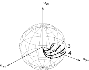
Figure 1: Time optimal realizations 40 of the entangler gate 58 with $\varphi=\frac{k\pi}{8}$, $k=1,2,3,4$, from the identity (origin) in the ${\boldsymbol{\alpha}}_{+}$-space. They are not geodesics.

V Case with fast operations

Let us now briefly discuss the quantum brachistochrone in the case where certain unitary operations have negligible time duration qit14tk . We assume that such operations (together with the unphysical global phase transformations) form a subgroup $K$ of the group $G=\operatorname{\it U}(N)$ of all the unitary operations. We denote the Lie algebras of $G$ and $K$ by ${\mathfrak{g}}$ and ${\mathfrak{k}}$, respectively. Note that the formulation in Section II can be considered as the special case of $K=\operatorname{\it U}(1)$.

In order to measure the time duration properly, we have to generalize the projection operator $P_{U}=P_{1}(AU^{\dagger})U$ in 2 so that $P_{1}$ is the orthogonal projection to ${\mathfrak{k}}$ in ${\mathfrak{g}}$, namely,

$$P_{1}(A):=\sum_{j}\langle g_{j},A\rangle g_{j},$$ (60)

where $\{g_{j}\}$ is an orthonormal basis for ${\mathfrak{k}}$. Apart from 60, the action 1 and the Lagrangian terms 2-4 are unchanged. Therefore, defining again $\widetilde{H}:=(1-P_{1})(H)$, we can repeat the same argument and obtain the same remaining equations of Section II and III. In particular, we obtain the quantum brachistochrone equation 16 and we can still follow the procedure (i)-(v) of Section II.

The terms $L_{T}$ and $L_{S}$ of the Lagrangian are now invariant under the (in general non-Abelian) gauge transformation

$$U\mapsto kU,\quad H\mapsto kHk^{\dagger}+i\dot{k}k^{\dagger},$$

$$\Lambda\mapsto k\Lambda k^{\dagger},\quad\lambda_{j}\mapsto\lambda_{j},$$ (61)

where $k(t)\in K$. Since $F$ transforms as $F\mapsto kFk^{\dagger}$ under V, the quantum brachistochrone equation 16 is always covariant, i.e., unchanged. Furthermore, if $L_{C}$ is invariant under V, the constraints are also gauge-invariant.

One of the systems which is often discussed in quantum computation is that of $n$ qubits in which the one-qubit operations take negligible time. This corresponds to the case $G=\operatorname{\it U}(2^{n})$ and $K=\operatorname{\it U}(1)\otimes\operatorname{\it SU}(2)^{\otimes n}$. Let ${{\mathfrak{g}}}_{j}$ be the subspace of ${{\mathfrak{g}}}$ representing infinitesimal $j$-qubit operations. Namely, ${{\mathfrak{g}}}_{j}$ consists of linear combinations of all the operators which are products of $j$ Pauli operators and $n-j$ identity operators:

$${{\mathfrak{g}}}_{j} :=\operatorname{span}_{\mathbb{R}}\{\sigma^{a_{1}\cdots a_{j}}_{l_{1}\cdots l_{j}};a_{1}<\cdots<a_{j}\text{ and }l_{j}=x,y,z\},$$

$$\qquad j\geq 0,$$ (62)

where $a_{m}$ represents the $a_{m}$th qubit for $m=1,\cdots,j$ and $\sigma^{a_{1}\cdots a_{j}}_{l_{1}\cdots l_{j}}$ is a generalization of $\sigma^{a}_{j}$ appearing in 29. For example, $\sigma^{13}_{xy}=\sigma_{x}\otimes 1\otimes\sigma_{y}\otimes 1\otimes\cdots\otimes 1$. Then we have ${\mathfrak{k}}={{\mathfrak{g}}}_{0}\oplus{{\mathfrak{g}}}_{1}$. Moreover, we can write 60 explicitly as $P_{1}=\sum_{j}P^{(j)}$ with

$$P^{(j)}(A):=\sum_{a_{1}<\cdots<a_{j}}\sum_{l_{1},\cdots,l_{j}}\sigma^{a_{1}\cdots a_{j}}_{l_{1}\cdots l_{j}}\operatorname{Tr}{\left(\sigma^{a_{1}\cdots a_{j}}_{l_{1}\cdots l_{j}}A\right)}/{2^{j}}.$$ (63)

Note that each $P^{(j)}$ is the orthogonal projection to ${{\mathfrak{g}}}_{j}$ in ${{\mathfrak{g}}}$.

Let us also assume that the infinitesimal operations including three or more qubits are not allowed in the Hamiltonian. This is the case of the linear homogeneous constraints discussed in Section III with $F^{\prime}=\sum_{j=3}^{n}F^{\prime}_{j}$, where

$$F^{\prime}_{j}:=\sum_{a_{1}<\cdots<a_{j}}\sum_{l_{1},\cdots,l_{j}}\lambda^{a_{1}\cdots a_{j}}_{l_{1}\cdots l_{j}}\sigma^{a_{1}\cdots a_{j}}_{l_{1}\cdots l_{j}}/{2^{j}},$$ (64)

and $\lambda^{a_{1}\cdots a_{j}}_{l_{1}\cdots l_{j}}$ are Lagrange multipliers. By choosing the gauge $H=\widetilde{H}$ we have $F^{\prime}_{j}\in{{\mathfrak{g}}}_{j}$, while from the constraints $f_{j}=0$ with $j\geq 3$ we get $\widetilde{H}\in{{\mathfrak{g}}}_{2}$. We find that the following commutation relations of the subspaces ${{\mathfrak{g}}}_{j}$ of the algebra ${{\mathfrak{g}}}$ hold:

$$[{{\mathfrak{g}}}_{j},{{\mathfrak{g}}}_{k}]={{\mathfrak{g}}}_{|j-k|+1}\oplus{{\mathfrak{g}}}_{|j-k|+3}\oplus\cdots\oplus{{\mathfrak{g}}}_{j+k-1},\quad j,k\geq 1,$$

$$[{{\mathfrak{g}}}_{0},{{\mathfrak{g}}}_{j}]=0,\quad j\geq 0,$$ (65)

where we understand that ${{\mathfrak{g}}}_{j}=0$ for $j>n$.

In particular, the three-qubit case, $n=3$, turns out to be simple and we can carry out the procedure in Section II up to (iv) in general qit14tk . In fact, by V we have $[{{\mathfrak{g}}}_{2},{{\mathfrak{g}}}_{3}]={{\mathfrak{g}}}_{2}$, and since $\widetilde{H}\in{{\mathfrak{g}}}_{2}$ and $F^{\prime}=F^{\prime}_{3}\in{{\mathfrak{g}}}_{3}$, the quantum brachistochrone equation 16 decouples into two equations

$$\dot{\widetilde{H}}=-i[\widetilde{H},F^{\prime}],\quad\dot{F}^{\prime}=0.$$ (66)

Thus we have $F^{\prime}(t)=F^{\prime}(0)$ and $\widetilde{H}(t)=e^{iF^{\prime}(0)t}\widetilde{H}(0)e^{-iF^{\prime}(0)t}$, so that we can drop the time ordering in 27, and we finally obtain

$$U(t)=e^{iF^{\prime}(0)t}e^{-i(\widetilde{H}(0)+F^{\prime}(0))t}.$$ (67)

A similar result was recently found in another setting dowling . Although the three-qubit system is particularly simple, the prescription (v) still remains technically involved. We postpone its full analysis to a future work.

VI Summary and discussion

We have studied the problem of finding the time optimal evolution of a unitary operator in $U(N)$ and the corresponding time optimal Hamiltonian within the context of a variational principle. Our main result is an explicit prescription for finding the time optimal unitary operation. Once the constraints for the available Hamiltonians are specified, the quantum brachistochrone equation can be immediately written down, and then the problem simply reduces to obtaining its solutions. Our formulation is general, systematic, and does not rely upon any restrictive assumptions, e.g., adiabaticity of quantum evolutions. We explicitly showed our methods and found the optimal Hamiltonian and the optimal time duration for three important examples of quantum gates acting on two qubits. The optimal Hamiltonians realizing the swap and qft gates are time independent and, therefore, the corresponding optimal unitary operators follow geodesic curves on the $SU(4)$ manifold endowed with the metric $ds_{\text{\tiny$U$}}^{2}$. This is not the case for the entangler gate (as expected for generic gates) where the optimal Hamiltonian is time dependent and the time evolution of the corresponding unitary operator is not geodesic. We also discussed the quantum brachistochrone for unitary operations in the case where there are operations whose time duration is negligible.

This work is a natural extension of our previous analysis of the time optimal evolution of quantum states in the projective space. The present formulation has direct relevance to quantum computation, since it gives the optimal realization of subroutines for unknown input states, e.g. the discrete Fourier transform. On the other hand, the quantum brachistochrone for state evolution in CarHosKoiOku06PRL may be viewed as a quantum computation for known initial states, e.g. the transition from $|00..0\rangle$ to a certain entangled state shor in Shor’s factorization algorithm.

We should caution the reader that, in order to make the variational principle well defined, the action 1 should be actually expressed as an integration over a parameter with fixed initial and final values. Since this does not affect our results, we have omitted these details for simplicity. Furthermore, we note that, instead of 2, any function of $i{\dot{U}}U^{\dagger}$ and $H$ which becomes constant upon using the Schrödinger equation would produce the same quantum brachistochrone equation 16. In this sense, the explicit expression of the metric in 2 does not affect our formulation. In a related work, the authors of nielsen1 , nielsen2 and nielsen3 rephrased the problem of finding efficient quantum algorithms in terms of the shortest path in a curved geometry. Their goal was to obtain a bound on the number of gates required to synthesize a given target unitary operation in terms of a cost function based on a certain metric in the space of Hamiltonians. By tailoring the form of such a metric they were able to approximate the target unitary operation by a circuit of size polynomial in the distance from the identity. On the other hand, our point of view here is that the time complexity of an algorithm is of more physical relevance than its gate complexity (see also, e.g. schulte ). Furthermore, although our result does not depend on the choice of the metric on $U(N)$, the bi-invariant metric 5 is the most natural. Also note that the simplest isotropic constraint 20 does not provide any non-trivial bound to the gate complexity. In our framework the general relationship between time and gate complexity is still an open issue.

Another point which we would like to emphasize is that, although what we treated here for the simplicity of exposition was the case in which the constraints are expressed as equality conditions for the functions $f_{j}(H)$, there should be no conceptual difficulty in extending our variational methods to the more realistic case when similar constraints are given in terms of inequalities (see. e.g., khun ).

Finally, we should note that the authors of khaneja , by using the Pontryagin maximal principle, also showed an optimal time dependent Hamiltonian as a particular solution to an equation which is similar to our quantum brachistochrone equation. In the two-qubit demonstration of our variational methods, we have obtained a general solution for the optimal Hamiltonian without attempting to match it to a prescribed NMR experiment, which was a main concern in khaneja . Our formalism also naturally allows for the treatment of the more general and physical situation in which one-qubit local controls require a non-zero time cost.

References

- [1] N. Khaneja and S.J. Glaser, Chem. Phys. 267, 11 (2001); N. Khaneja, R. Brockett and S.J. Glaser, Phys. Rev. A63, 032308 (2001).
- [2] G. Vidal, K. Hammerer and J.I. Cirac, Phys. Rev. Lett. 88, 237902 (2002); id., Phys. Rev. A66, 062321 (2002); J. Zhang, J. Vala, S. Sastry and K.B. Whaley, Phys. Rev. A67, 042313 (2003).
- [3] T. Schulte-Herbrüggen, A. Spörl, N. Khaneja and S.J. Glaser, Phys. Rev. A72, 042331 (2005).
- [4] U. Boscain and P. Mason, J. Math. Phys. 47, 062101 (2006).
- [5] M.A. Nielsen and I.L. Chuang, Quantum Computation and Quantum Information (Cambridge University Press, Cambridge, 2000).
- [6] S. Tanimura, M. Nakahara and D. Hayashi, J. Math. Phys. 46, 022101 (2005).
- [7] A. Carlini, A. Hosoya, T. Koike, and Y. Okudaira, Phys. Rev. Lett. 96, 060503 (2006).
- [8] M.A. Nielsen, M. Dowling, M. Gu and A. Doherty, Science 311, 1133 (2006).
- [9] M.A. Nielsen, M.R. Dowling, M. Gu and A.C. Doherty, quant-ph/0603160.
- [10] N. Khaneja, B. Heitmann, A. Spörl, H. Yuan, T. Schulte-Herbrüggen and S.J. Glaser, quant-ph/0605071.
- [11] This equation is characteristic of time optimality and not of, e.g., fidelity optimality (see J.P. Palao and R. Kosloff, Phys. Rev. A68, 062308 (2003) and references therein).
- [12] in preparation.
- [13] The definition of in [7], i.e. Equation (17) there, is different from 12 of the present paper. However, one can easily show that Equation (16) in [7] is, with the help of (15) there and the Schrödinger equation, equivalent to the quantum brachistochrone equation 16 in the present paper with the present definition of .
- [14] For example, a tunable spin-spin coupling can be physically realized through superconducting flux qubits (A.O. Niskanen, Y. Nakamura and J.-S. Tsai, Phys. Rev. B73, 094506(2006)).
- [15] A. Messiah, Quantum Mechanics (Dover, 1999).
- [16] P.W. Shor, Proc. 35th Ann. Sym. Found. Comp. Sci., 124 (IEEE Computer Society Press, New York, 1994).
- [17] M.A. Nielsen, Quant. Inf. Comput. 6, 213 (2006).
- [18] D.P. Bertsekas, Nonlinear Programming (Athena Scientific, 1999).
- [19] A. Carlini, A. Hosoya, T. Koike, and Y. Okudaira, “Time-optimal quantum evolution”, Proceedings of the Workshop on QIT 14 at Tokyo Institute of Technology, May 2006.
- [20] M. Dowling and M. A. Nielsen, quant-ph/0701004.