Quantum Control of a Single Qubit

Abstract

Measurements in quantum mechanics cannot perfectly distinguish all states and necessarily disturb the measured system. We present and analyse a proposal to demonstrate fundamental limits on quantum control of a single qubit arising from these properties of quantum measurements. We consider a qubit prepared in one of two non-orthogonal states and subsequently subjected to dephasing noise. The task is to use measurement and feedback control to attempt to correct the state of the qubit. We demonstrate that projective measurements are not optimal for this task, and that there exists a non-projective measurement with an optimum measurement strength which achieves the best trade-off between gaining information about the system and disturbing it through measurement back-action. We study the performance of a quantum control scheme that makes use of this weak measurement followed by feedback control, and demonstrate that it realises the optimal recovery from noise for this system. We contrast this approach with various classically inspired control schemes.

I Introduction

Any practical quantum technology, such as quantum key distribution or quantum computing, must function robustly in the presence of noise. Many modern “classical” technologies tolerate noise, faulty parts, etc., by relying on feedback control systems, which monitor the system and use this information to control its state. Given the ubiquity and power of feedback control for classical systems, it is worthwhile investigating how such control concepts can be applied to quantum technologies as well. However, strategies for quantum control must take into account some fundamental features of quantum mechanics, namely, restrictions on information gain, and measurement back-action.

Classically, it is possible in principle to acquire all the information about the state of a system with certainty by using sufficiently precise measurements. That is, the state of a single classical system can be precisely determined via measurement. For quantum systems, however, this is not always possible: if the system is prepared in one of several non-orthogonal states, no measurement can determine which preparation occurred with certainty.

In addition, for quantum systems, monitoring comes at a price: any measurement that acquires information about a system must necessarily disturb it uncontrollably. This feature is often referred to as back-action — the fundamental noise induced on a system through any measurement, which maintains the uncertainty relations. This feature of quantum measurement is also distinct from the classical situation, wherein measurements that do not alter the state of the system can in principle be performed.

These two fundamental features of quantum systems — that non-orthogonal states cannot be perfectly discriminated, and that any information gain via measurement necessarily implies disturbance to the system — require a reevaluation of conventional methods and techniques from control theory when developing the theory of quantum control.

In this paper, we investigate the use of measurement and feedback control of a single qubit, prepared in one of two non-orthogonal states and subsequently subjected to noise. Our main result is that, in order to optimize the performance of the control scheme (as quantified by the average fidelity of the corrected state compared to the initial state), one must use non-projective measurements with a strength that balances the trade-off between information gain and disturbance.

Belavkin was the first to recognise the importance of feedback control for quantum systems and describe a theoretical framework for analysing both discrete and continuous time models Belavkin (1983, 1999). Despite this early start, it is only recently that the degree of control and isolation of quantum systems has progressed to the point that the experimental exploration of quantum control tasks has been possible Armen et al. (2002); Smith et al. (2002); Geremia et al. (2004); Reiner et al. (2004); LaHaye et al. (2004); Bushev et al. (2006), and the field is now undergoing rapid development (see for example 05j (2005)).

The specific control problem we are interested in here is the stabilization against noise of states of a single two level system. Similar problems have been considered in continuous time feedback models, e.g., the stabilization of a single state of a driven and damped two-level atom Wang and Wiseman (2001); Wiseman et al. (2002) and the maintenance of the coherence of a qubit undergoing decoherence Lidar and Schneider (2005). Several recent papers have investigated state preparation and feedback stabilization onto eigenstates of a continuously-measured observable in higher-dimensional systems van Handel et al. (2005); Mirrahimi and van Handel . In contrast to these prior investigations, we investigate a feedback scheme to stabilize two non-orthogonal states of a two-level system. We work in a discrete-time setting, rather than continuous-time as considered in most prior work, which considerably simplifies the problem and most clearly illustrates the central concepts. Gregoratti and Werner have investigated exactly this kind of model of recovering the state of the system after interaction with the environment Gregoratti and Werner (2003, 2004) in the case where it is possible to make measurements on the environment. In our setting we imagine that the environment that causes the initial decoherence is not available subsequently for the feedback protocol. Our main interest is to investigate the effects of the kind of trade-off between information and disturbance that is ubiquitous in quantum information in a concrete optimal control problem. Related information-disturbance trade-offs in quantum feedback control are discussed in Doherty et al. (2001). Finally, we note that implementing quantum operations on a single qubit through the use of measurement and feedback control as considered here has been investigated for eavesdropping strategies in quantum cryptography Niu and Griffiths (1999) and for engineering general open-system dynamics Lloyd and Viola (2001).

Note that there is a fundamental difference between the kind of quantum control problem we are considering here and the related task of quantum error correction. (For an introduction to the latter, see Nielsen and Chuang (2000).) The essence of quantum error correction is to encode abstract quantum information into a physical quantum system and to choose degrees of freedom that are unaffected by the relevant noise, or upon which errors can be deterministically corrected. However, it can be the case that one wishes to protect particular physical degrees of freedom of quantum systems and one is not free to choose an arbitrary encoding. (One such example is reference frame distribution via the exchange of quantum systems). The quantum states required for these schemes cannot be encoded into quantum error correcting codes or noiseless subsystems Preskill (2000); protecting such systems from noise may therefore be an application of this kind of quantum control.

The paper is structured as follows. In section II, we define the control task in detail; in section III, we present and determine the performance of control strategies based on “classical” concepts. Section IV introduces our quantum strategy, investigating the use of weak quantum measurements, and analyses its performance against the strategies of section III. We also demonstrate that our quantum control scheme is optimal for the task at hand. In section V we discuss the implications of our result and their relevance to other problems.

II A Simple Control Task

The aim of this paper is to explore the key issues we will confront when applying concepts from control theory to finite-dimensional quantum systems. In order to facilitate the analysis and to be able to concentrate on the key departures from classical control, we will chose a very simple quantum system and noise model. The emphasis is not towards a practical task, but as an illustrative example.

Consider the following operational task: a qubit prepared in one of two non-orthogonal states $|\psi_{1}\rangle$ or $|\psi_{2}\rangle$ (with overlap $\langle\psi_{1}|\psi_{2}\rangle=\cos\theta$ for $0\leq\theta\leq\pi/2$) is transmitted along a noisy quantum channel. Without knowing which state was transmitted, we will attempt to “correct” the system, i.e., undo the effect of the noise, through the use of a control scheme based on measurement and feedback; see Fig. 1.

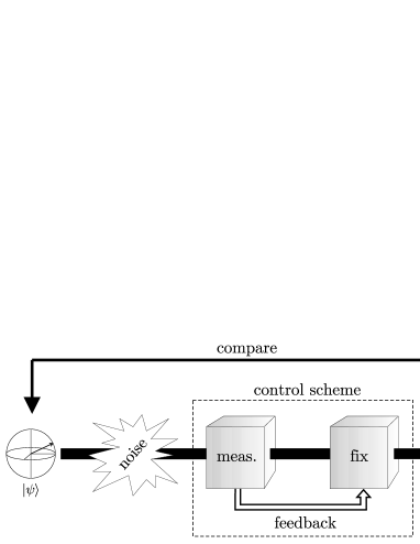
Figure 1: Schematic of a quantum control procedure. A qubit, subjected to dephasing noise, is subsequently measured and corrected based on the results of this measurement. The output state $\rho$ is compared with the input state $|\psi\rangle$ to characterise how well the scheme performs.

The noise model that we will consider is dephasing noise. Let $\{|0\rangle,|1\rangle\}$ be a basis for the qubit Hilbert space, and the Pauli operator $Z$ is the unitary operator defined by $Z|0\rangle=|0\rangle$, $Z|1\rangle=-|1\rangle$. Dephasing noise is characterized as follows: with probability $p$ a phase-flip $Z$ is applied to the system, and with probability $1-p$ the system is unaltered. The noise is thus described by a quantum operation Nielsen and Chuang (2000), i.e., a completely-positive trace-preserving (CPTP) map $\mathcal{E}_{p}$, that acts on a single-qubit density matrix $\rho$ as

$$\mathcal{E}_{p}(\rho)=p(Z\rho Z)+(1-p)\rho\,.$$ (1)

We will consider the noisy channel to be fully characterized, meaning that $p$ is known and without loss of generality in the range $0\leq p\leq 0.5$.

We will choose the two initial states to be oriented in such a way that their distinguishability, as measured by their trace distance, is maintained under the action of the noise. It is straightforward to show that this condition is satisfied by the states

$$|\psi_{1}\rangle =\cos\tfrac{\theta}{2}|{+}\rangle+\sin\tfrac{\theta}{2}|{-}\rangle\,,$$ (2)

$$|\psi_{2}\rangle =\cos\tfrac{\theta}{2}|{+}\rangle-\sin\tfrac{\theta}{2}|{-}\rangle\,,$$ (3)

where $|{\pm}\rangle=(|0\rangle\pm|1\rangle)/\sqrt{2}$.

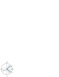
Figure 2: Bloch sphere representation of the initial states, and the states after the noise. The noise shortens the Bloch vectors along the $x$-axis. We have used the notation $\mathcal{E}(\psi)$ as a shorthand for $\mathcal{E}(|\psi\rangle\langle\psi|)$.

Consider the Bloch sphere defined by states $|0\rangle$ and $|1\rangle$ as the poles on the $z$-axis. The two states $|\psi_{1}\rangle$ and $|\psi_{2}\rangle$ lie in the $x{-}z$ plane and straddle the equator of the Bloch sphere by angles $\pm\theta$; see Fig. 2. On this Bloch sphere, the dephasing noise acting on these states has the effect of decreasing the $x$-component of their Bloch vectors. The trace distance between these two states, given by the Euclidean distance between their Bloch vectors, is invariant under this dephasing noise.

We now consider whether there exists a control procedure $\mathcal{C}$ (some “black box”) that can correct the state of this system and counteract the noise, at least to some degree, independent of which input state was prepared. To quantify the performance of any such procedure, we will use the average fidelity to compare the noiseless input states $|\psi_{i}\rangle$ with the corrected output states $\rho_{i}$. Assuming an equal probability for sending either state $|\psi_{1}\rangle$ or $|\psi_{2}\rangle$, the figure of merit is

$$F_{\mathcal{C}} =\tfrac{1}{2}F(|\psi_{1}\rangle,\rho_{1})+\tfrac{1}{2}F(|\psi_{2}\rangle,\rho_{2})$$

$$=\tfrac{1}{2}\langle\psi_{1}|\rho_{1}|\psi_{1}\rangle+\tfrac{1}{2}\langle\psi_{2}|\rho_{2}|\psi_{2}\rangle\,,$$ (4)

where the fidelity between a pure state $|\psi\rangle$ and a mixed state $\rho$ is defined as $F(|\psi\rangle,\rho)\equiv\langle\psi|\rho|\psi\rangle$. The fidelity $F$ ranges from 0 to 1 and is a measure of how much two states overlap each other (a fidelity of 0 means the states are orthogonal, whereas a fidelity of 1 means the states are identical). It has the following simple operational meaning when the input state is pure: the fidelity $F(|\psi_{i}\rangle,\rho_{i})$ is the probability that the state $\rho_{i}$ will yield outcome $|\psi_{i}\rangle$ from the projective measurement $\{|\psi_{i}\rangle\langle\psi_{i}|,|\psi_{i}^{\perp}\rangle\langle\psi_{i}^{\perp}|\}$.

Thus, the aim is to find a control operation, described by a CPTP map $\mathcal{C}$ independent of the choice of initial state, such that the corrected states

$$\rho_{i}=\mathcal{C}\bigl{[}\mathcal{E}_{p}(|\psi_{i}\rangle\langle\psi_{i}|)\bigr{]}\,,$$ (5)

for $i=1,2$ are close to the original states as quantified by the average fidelity. We consider control operations that consist of two steps: a measurement on the quantum system, followed by a feedback operation that is conditioned on the measurement result, as shown in Fig. 1.

III Classical Control

In this section, we introduce two types of control schemes for this task, both of which are based on classical concepts, and we calculate the performance of these schemes based on the average fidelity. In Sec. IV, we will introduce a quantum control scheme that outperforms both of these classical schemes.

Classical Strategy A: Discriminate and Reprepare

For the control of classical systems, it is always advantageous to acquire as much information about the system as possible in order to implement the best feedback scheme. In line with this principle, a possible control strategy would be to perform a measurement on the system which attempts to discriminate between the input states, and then to reprepare the system in some state based on the measurement result.

We first characterize all possible discriminate-and-reprepare schemes; such schemes are associated with entanglement breaking trace preserving (EBTP) maps Horodecki et al. (2003); Ruskai (2003), as follows. Any discrimination step is described by a generalized measurement, (or positive operator-valued measure (POVM)) Nielsen and Chuang (2000) yielding a classical probability distribution. The generalized measurement is described by the operators $\{P_{a}\}$ with $P_{a}\geq 0$ and $\sum_{a}P_{a}=I$. The resulting map on the quantum system is called a quantum-classical map $QC$ Holevo (1998), given by

$$QC(\rho)=\sum_{a}{{\rm Tr}\left[\rho P_{a}\right]|e_{a}\rangle\langle e_{a}|}\,,$$ (6)

where $\{|e_{a}\rangle\}$ is an orthonormal basis. The reprepare step, in which the quantum system is re-prepared based on the classical measurement outcome, is described by a classical-quantum map $CQ$ Holevo (1998), given by

$$CQ(\rho)=\sum_{b}{{\rm Tr}\left[\rho|e_{b}\rangle\langle e_{b}|\right]Q_{b}}\,,$$ (7)

where $\{Q_{b}\}$ are density matrices.

The concatenation $(CQ\circ QC)(\rho)$ leads to a map of the form

$$\mathcal{B}(\rho)=\sum_{b}{{\rm Tr}\left[\rho P_{b}\right]Q_{b}}\,.$$ (8)

This map is an entanglement breaking channel. The name arises because the output system is unentangled with any other system, regardless of its input state. In fact it is straightforward to see from Horodecki et al. (2003); Ruskai (2003) that all EBTP maps can be realised by some discriminate-and-reprepare scheme. Thus these EBTP maps formalize our notion of discriminate-and-reprepare strategies.

The measurement for discriminating two (possibly mixed) preparations given by Helstrom Helstrom (1976) is optimal in terms of maximizing the average probability of a success. For our choice of states, Helstrom’s measurement is a projective measurement onto the basis $\{|0\rangle,|1\rangle\}$, which successfully discriminates the states $|\psi_{1}\rangle$ and $|\psi_{2}\rangle$ with probability $P_{\rm Helstrom}=\frac{1}{2}(1+\sin\theta)$. Note that because of the particular choice of dephasing noise, this success probability is independent of the noise strength $p$.

We now present and analyse two possible discriminate-and-reprepare strategies, both of which are based on Helstrom’s measurement.

Discriminate and Reprepare Scheme 1:

With the outcome of Helstrom’s measurement, one strategy is to reprepare the qubit in either state $|\psi_{1}\rangle$ or $|\psi_{2}\rangle$ based on this measurement outcome. This scheme yields an average fidelity of

$$F_{\rm DR1}=1-\tfrac{1}{2}\left(\sin^{2}{\theta}-\sin^{3}{\theta}\right)\,.$$ (9)

Such a replacement ignores the fact that the discrimination step can fail, with probability $1-P_{\rm Helstrom}$, in which case a prepared state $|\psi_{1}\rangle$ would be reprepared as $|\psi_{2}\rangle$ (or vice versa).

Discriminate and Reprepare Scheme 2:

We can consider other strategies that reprepare different states so as to reduce the effect of the aforementioned error. In particular, we now demonstrate that the following pair of states maximises the average fidelity:

$$|\Psi_{\pm}\rangle=\sqrt{\tfrac{1}{2}\pm\tfrac{\sin^{2}{\theta}}{2\gamma}}|0\rangle+\sqrt{\tfrac{1}{2}\mp\tfrac{\sin^{2}{\theta}}{2\gamma}}|1\rangle\,,$$ (10)

where $\gamma\equiv\sqrt{\sin^{4}{\theta}+\cos^{2}{\theta}}$. Note that this replacement is also independent of $p$. Here, $|\Psi_{+}\rangle$ is prepared if the measurement outcome corresponds to $|\psi_{1}\rangle$, and $|\Psi_{-}\rangle$ is prepared otherwise. In this strategy, the reprepared states are slightly biased towards the alternate state to that suggested by the measurement (smaller $\theta$) — in a sense hedging our bet. As a proof of the superiority of this scheme over the former, the fidelity

$$F_{\rm DR2}=\frac{1}{2}+\frac{1}{2}\sqrt{\cos^{2}{\theta}+\sin^{4}{\theta}}\,,$$ (11)

satisfies $F_{\rm DR2}\geq F_{\rm DR1}$ for all $\theta$. Both $F_{\rm DR1}$ and $F_{\rm DR2}$ are presented in Fig. 3(a).

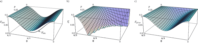
Figure 3: The performance of the schemes, quantified by the average fidelity, as a function of the amount of noise $p$ and the angle between the input states $\theta$. a) Discriminate and reprepare scheme quantified by the average fidelity $F_{\rm DR2}$ of Eq. (11). The fidelity $F_{\rm DR1}$ of Eq. (9) is shown as a solid line at $p=0.5$. Both average fidelities $F_{\rm DR2}$ and $F_{\rm DR1}$ are independent of $p$. b)“Do nothing” scheme, quantified by the average fidelity $F_{\rm N}$ of Eq. (13). For this scheme, the average fidelity drops to $F_{\textrm{N}}=1/2$ for $p=0.5$ and $\theta=0$. c) Quantum control scheme, quantified by the average fidelity $F_{\mathrm{QCopt}}$ of Eq. (27). The range of fidelities plotted has been made identical in all the figures to aid comparison.

This second discriminate-and-reprepare scheme is in fact the optimal discriminate-and-reprepare scheme, in that it achieves the highest average fidelity

$$\max_{\mathcal{B}}F_{\mathcal{B}}=\max_{\mathcal{B}}\tfrac{1}{2}\sum_{i=1}^{2}{\langle\psi_{i}|\mathcal{B}\bigl{[}\mathcal{E}_{p}(|\psi_{i}\rangle\langle\psi_{i}|)\bigr{]}|\psi_{i}\rangle}\,,$$ (12)

where the maximization is over all EBTP maps $\mathcal{B}$ acting on a single qubit. This optimization was performed (in a different setting) by Fuchs and Sasaki Fuchs and Sasaki (2003). In the Appendix, we provide an alternate proof of optimality using techniques from convex optimization.

Classical Strategy B: Do Nothing

Another control strategy would be to do nothing to correct the states. Although trivial, this strategy is of interest for comparison with other schemes. (There exist schemes that perform worse than this strategy, because of the feature of quantum systems that every measurement that acquires information will uncontrollably disturb the system.) This scheme does not lie within the set of discriminate-and-reprepare schemes described above (it is not described by an EBTP map) but we will nonetheless refer to it as “classical.”

The average fidelity of this scheme is given by

$$F_{\rm N}=1-p\cos^{2}\theta\,.$$ (13)

This performance is plotted in Fig. 3(b). Clearly, this scheme performs best for small amounts of noise ($p\simeq 0$) and for input states with Bloch vectors that are near the $z$-axis (which is invariant under the dephasing noise). In some non-trivial regions of the $(p,\theta)$ parameter space, in particular in the range of low noise, this “do nothing” scheme outperforms the optimal “discriminate and reprepare” scheme.

IV Quantum Control

In the previous section, we presented control schemes based on classical concepts. However, using techniques that may lead to optimal control schemes for a classical system may not necessarily lead to optimal schemes for a quantum system. As we will now demonstrate, the above classical control strategies can be outperformed by using a strategy based on quantum concepts.

We note that the two classical schemes presented in the previous section lie at the extreme ends of a spectrum: the “discriminate-and-reprepare” strategy achieved maximum information gain and induced a maximum disturbance, whereas the “do-nothing” strategy achieved zero disturbance but produced zero information gain. As demonstrated by Fuchs and Peres Fuchs and Peres (1996), there exist an entire range of generalized measurements that trade off information gain and disturbance. A possible avenue for improvement in our control schemes is to tailor the measurement in such a way as to find a compromise, if one exists, between acquiring information about the noise but not disturbing the system too much as a result of the measurement.

In the following we re-express the noise process $\mathcal{E}_{p}$ in a way that suggests a strategy for constructing such an improved feedback protocol.

IV.1 Reexpressing the noise

To develop an intuitive picture, we will make use of a preferred ensemble for the quantum operation $\mathcal{E}_{p}$ describing the noise. That is, we use a decomposition of the operation into different Kraus (error) operators than that given in Eq. (1). The resulting quantum operation $\mathcal{E}_{p}$ describing the noise, however, is equivalent.

Consider the following quantum operation on a qubit, viewed on the Bloch sphere: with probability $1/2$, the Bloch vector of the qubit is rotated by an angle $+\alpha$ about the $z$-axis, and with probability $1/2$ it is rotated by $-\alpha$ about the $z$-axis. Rotations about the $z$-axis are described by the operator

$$Z_{\alpha}=\mathrm{e}^{-i\alpha Z/2}=\cos(\alpha/2)I-i\sin(\alpha/2)Z\,,$$ (14)

and the quantum operation is then

$$\mathcal{E}_{\alpha}(\rho) =\tfrac{1}{2}Z_{\alpha}\rho Z_{\alpha}^{\dagger}+\tfrac{1}{2}Z_{-\alpha}\rho Z_{-\alpha}^{\dagger}$$

$$=\sin^{2}(\alpha/2)(Z\rho Z)+\cos^{2}(\alpha/2)\rho\,.$$ (15)

Thus, this quantum operation is equivalent to the dephasing noise $\mathcal{E}_{p}$, with $p=\sin^{2}(\alpha/2)$.

Viewing the noise operation $\mathcal{E}_{p}$ with this preferred ensemble, it is possible to describe the noise as rotating the Bloch vector of the state by $\pm\alpha$ with equal probability. A possible control strategy, then, would be to attempt to acquire information about the direction of rotation ($\pm\alpha$) via an appropriate measurement, and then to correct the system based on this estimate. Loosely, we desire a measurement that determines whether the noise rotated the state one way ($+\alpha$) or another ($-\alpha$). Then, based on the measurement result, we apply feedback: a unitary operation (rotation) that takes the state of the system back to the desired axis.

A projective measurement, wherein the state of the system collapses to an eigenstate of the measurement, does not meet these requirements because such a measurement destroys the distinguishability of the two possible states. Instead, we consider the use of a weak measurement, with a measurement strength chosen to balance the competing goals of acquiring information and leaving the system undisturbed. We now show that such a strategy is possible, and that there is a non-trivial optimal measurement strength for this task.

IV.2 Weak non-destructive measurements

For our quantum control scheme, we will make use of a type of measurement that satisfies two key requirements: (1) the strength of the measurement should be controllable, i.e., we should be able to vary the trade-off between information gain and disturbance (back-action); and (2) the measurement should be non-destructive, which leaving the measured system in an appropriate quantum state given by the desired collapse map. Such weak non-destructive measurements have recently been developed and demonstrated in single-photon quantum optical systems Pryde et al. (2004); Ralph et al. (2006).

Using the preferred ensemble describing the noise, Eq. (15), we expect intuitively that this weak measurement should be along the $y$-axis of the Bloch sphere in order to provide information about which direction ($\pm\alpha$) the system was rotated, without acquiring information about which initial state the system was prepared in. One suitable family of POVMs consists of two operators given by $E_{m}=M_{m}^{\dagger}M_{m}$, for $m=0,1$, where $M_{m}$ are the measurement operators Nielsen and Chuang (2000)

$$M_{0} =\cos(\chi/2)|{+}i\rangle\langle{+}i|+\sin(\chi/2)|{-}i\rangle\langle{-}i|\,,$$ (16)

$$M_{1} =\sin(\chi/2)|{+}i\rangle\langle{+}i|+\cos(\chi/2)|{-}i\rangle\langle{-}i|\,.$$ (17)

The strength of the measurement depends on the choice of the parameter $\chi$. The eigenstates of $Y$ are $|{\pm}i\rangle\equiv(|0\rangle\pm i|1\rangle)/\sqrt{2}$. The probabilities of obtaining the measurement results $m=0,1$ for a qubit in the state $\rho_{\rm in}$ are given by

$$p_{m}=\text{Tr}[E_{m}\rho_{\rm in}]\,,$$ (18)

and the resulting state of the qubit immediately after the measurement is

$$\rho_{\rm out}^{(m)}=\frac{M_{m}\rho_{\rm in}M_{m}^{{\dagger}}}{p_{m}}\,.$$ (19)

Consider the following two limits. If $\chi=\pi/2$ the two measurement operators are the same and are proportional to the identity. As a result the outcome probabilities are independent of the state and the state of the signal is unaltered by the measurement. If $\chi=0$, a projective measurement on the signal is induced: the signal state is projected onto the state $|{{-}i}\rangle$ ($|{{+}i}\rangle$) when the measurement result is 0 (1). For $0<\chi<\pi/2$, the resulting measurement on the signal is non-projective but non-trivial.

It is illustrative to view the effect of this measurement on the noisy input states on the Bloch sphere. In Fig. 4(a) we can see that the effect of the noise is to shorten the length of the Bloch vector of the qubit state (making it less pure) while increasing the angle between the Bloch vector and the $x$-$y$ plane from $\theta$ to $\theta^{\prime}$, where $\theta^{\prime}>\theta$ . When the measurement is made, three things happen, as can be seen in Fig. 4(b): 1) the Bloch vector is lengthened (the state becomes more pure); 2) the angle $\theta^{\prime}$ decreases to some lesser angle $\theta^{\prime\prime}$; and 3) the state is rotated about the $z$-axis one way or the other depending on the result of the measurement. The first two effects work towards our advantage (purifying the state while decreasing $\theta^{\prime}$); the third effect we attempt to correct using feedback.

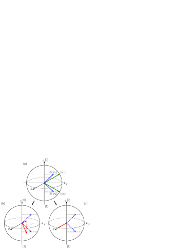
Figure 4: Bloch sphere representation of the effect of a weak measurement on the system. The transformations shown here correspond to having obtained the measurement result “$0$” (for the result “$1$”, the behaviour would be a reflection in the $x$-$z$ plane.) a) The two initial states $|\psi_{1,2}\rangle$ are mapped to $\rho_{1,2}$ by the noise; b) a weak measurement is performed with $0<\chi<\frac{\pi}{2}$; c) a strong projective measurement ($\chi=0$) is performed projecting either state into $|{{-}i}\rangle$. While no measurement will not yield any information about the system, a strong measurement will maximally disturb the system. A weak measurement will gain some information while also limiting the disturbance on the system.

We will now describe how to implement this measurement using a projective measurement on an ancillary meter qubit and an entangling gate between the original signal qubit and the meter. The strength of the measurement can be controlled by varying the level of entanglement between the two qubits, which can be implemented by initiating the meter in the state $|0\rangle$ and subsequently applying a $Y_{\chi}$ rotation (as shown in figure 5(a)), where

$$Y_{\chi}=\mathrm{e}^{-i\chi Y/2}=\begin{pmatrix}\cos(\chi/2)&-\sin(\chi/2)\\ \sin(\chi/2)&\cos(\chi/2)\end{pmatrix}\,.$$ (20)

The parameter $\chi$ ranges from $0$ to $\pi/2$ and characterises the strength of the measurement, with 0 equivalent to a projective measurement and $\pi/2$ equivalent to no measurement.

The entangling gate consists of a $X_{\frac{\pi}{2}}$ rotation on the signal state, followed by a cnot gate with the signal state as the control and the meter state as the target, followed by a $X_{-\frac{\pi}{2}}$ on the signal state, where

$$X_{\phi}=\mathrm{e}^{-i\phi X/2}=\begin{pmatrix}\cos(\phi/2)&-i\sin(\phi/2)\\ -i\sin(\phi/2)&\cos(\phi/2)\end{pmatrix}\,,$$ (21)

and where the Pauli matrix $X$ is given by $X|0\rangle=|1\rangle$ and $X|1\rangle=|0\rangle$. The rotations $X_{\pm\frac{\pi}{2}}$ are used to ensure that the resulting weak measurement on the signal qubit is performed in the $\{|{+}i\rangle,|{-}i\rangle\}$ basis. The entangling gate then correlates (to a degree which depends on $\chi$) the $\{|{+}i\rangle,|{-}i\rangle\}$ basis of the signal qubit to the $\{|0\rangle,|1\rangle\}$ basis of the meter qubit.

a)

b)

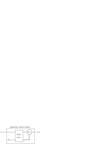
Figure 5: a) Circuit diagram of the weak measurement scheme. The input signal state $\rho_{\rm in}$ is entangled to the meter state using the cnot gate. The $X_{\pm\frac{\pi}{2}}$ rotations ensure that the weak measurement of the signal state is made in the desired basis $\{|{+}i\rangle,|{-}i\rangle\}$. The strength of the measurement is set using the rotation $Y_{\chi}$. The meter state is measured in the computational basis, resulting in a classical signal (0 or 1) to be fed forward to the correction stage of the control scheme.
b) Circuit diagram of the control scheme. A weak measurement is made on the input state and, based on the measurement results, the signal state will be rotated by $Z_{\eta}$ ($Z_{{-}\eta}$) conditional on the result of the weak measurement being 0 (1).

Finally the meter qubit is measured in the basis $\{|0\rangle,|1\rangle\}$, yielding a result 0 or 1. This measurement on the meter induces a measurement on the signal that is precisely equal to the generalized measurement described by the measurement operators $M_{m}$ of Eq. (16).

IV.3 Feedback control

Once a weak measurement has been performed, a correction based on the measurement result is performed on the quantum system: the feedback control. We choose the correction to be a unitary rotation about the $z$-axis, $Z_{\pm\eta}$ where

$$Z_{\eta}=\mathrm{e}^{-i\eta Z/2}=\begin{pmatrix}\mathrm{e}^{-i\eta/2}&0\\ 0&\mathrm{e}^{+i\eta/2}\end{pmatrix}\,,$$ (22)

with the aim to bring the Bloch vector of the qubit back onto the $xz$-plane. The angle of rotation is chosen to be $\pm\eta$, depending on the measurement result (${+}\eta$ corresponding to the measurement result 0, and ${-}\eta$ to the measurement result 1). It is possible to choose $\eta$ so that the system state is returned to the $xz$-plane for all values of $p,\theta$ and $\chi$ and for both measurement outcomes by choosing

$$\tan\eta=\frac{1}{(1-2p)\cos\theta\tan\chi}\,,$$ (23)

with $\eta$ in the range $0\leq\eta\leq\pi/2$. This angle $\eta$ can be calculated because the dephasing noise has been previously characterised (i.e., $p$ is known).

The resulting weak measurement followed by feedback is thus described by a quantum operation (a CPTP map) $\mathcal{C}_{\rm QC}$ acting on a single qubit, given by

$$\mathcal{C}_{\rm QC}(\rho)=(Z_{{+}\eta}M_{0})\rho(Z_{{+}\eta}M_{0})^{\dagger}+(Z_{{-}\eta}M_{1})\rho(Z_{{-}\eta}M_{1})^{\dagger}\,,$$ (24)

where the measurement operators $M_{m}$ are given by Eqs. (16-17).

In summary, the quantum control scheme operates by performing a weak measurement of the system and then correcting it based on the results of the measurement, as in Fig. 5b). The weak measurement is made by entangling an ancillary meter state with the signal state using an entangling unitary operation, then performing a projective measurement of the meter state. The level of entanglement depends on the input state of the meter, which is controlled by a $Y_{\chi}$ rotation; this level of entanglement in turn determines the strength of the measurement. After measurement of the meter, the signal state is altered due to the measurement back-action. To correct for this back-action, a rotation about the $z$-axis is applied to the state, returning it back to the $xz$-plane. To characterise how well the scheme works, we now investigate the average fidelity.

IV.4 Performance

The performance of this quantum control scheme, quantified by the average fidelity (II), is

$$F_{\mathrm{QC}}=\tfrac{1}{2}\left[1+\sin^{2}\theta\sin\chi+\cos\theta\sqrt{1-(1-r_{x}^{2})\sin^{2}\chi}\right]\,,$$ (25)

where $r_{x}=(1-2p)\cos{\theta}$ is the $x$ component of the Bloch vector describing the system after the noise.

We can see that $F_{\mathrm{QC}}$ is a function of the amount of noise $p$, the angle between the initial states $\theta$, and the measurement strength $\chi$. The dependence of this fidelity on the measurement strength, for fixed $p$ and $\theta$, is illustrated in Fig. 6. For each value of $p$ and $\theta$, there is an optimum measurement strength $\chi_{\mathrm{opt}}$ which maximizes the average fidelity (25). This optimum measurement strength is found to be non-trivial except for the limiting cases of $p=0$ or $\theta=0,\pi/2$, and is given by

$$\chi_{\rm opt}(p,\theta)\equiv\sin^{-1}\sqrt{\frac{\sin^{4}\theta}{(1-r_{x}^{2})^{2}\cos^{2}\theta+(1-r_{x}^{2})\sin^{4}\theta}}\,,$$ (26)

as a function of the amount of noise $p$ and the angle between the initial states $\theta$.

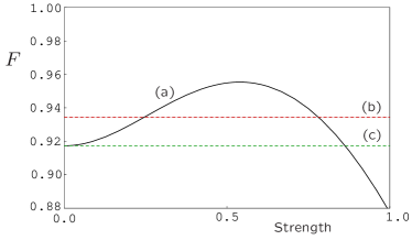
Figure 6: (a) Fidelity of the quantum correction procedure with measurement strength ($1-2\chi/\pi$) for a representative noise value ($p=0.145$) and angle ($\theta=0.715$). The measurement strength ranges from a value of 0 (corresponding to no measurement), through to a value of 1 (corresponding to a projective measurement). There exists an optimum measurement strength at which we balance the amount of information gained with the amount of back-action noise introduced. Also plotted for comparison are (b) the optimal “discriminate-and-reprepare” scheme and (c) the “do nothing” scheme for the same parameter values.

Substituting $\chi_{\mathrm{opt}}$ for $\chi$ in Eq. (25), we get the following expression for the optimum fidelity:

$$F_{\mathrm{QCopt}}=\tfrac{1}{2}+\tfrac{1}{2}\sqrt{\cos^{2}\theta+\frac{\sin^{4}\theta}{1-r_{x}^{2}}}\,.$$ (27)

Fig. 3(c) plots the quantum control fidelity as a function of the input state (characterised by the angle $\theta$) and the amount of noise (characterised by $p$).

We note that $F_{\mathrm{QCopt}}=1$ for three limiting cases. If $p=0$, there is no noise and so the state is not perturbed, resulting in unit fidelity for all values of $\theta$ given by simply “doing nothing” (zero measurement strength and no feedback). When $\theta=\pi/2$, the states are orthogonal and point along the $z$ axis. The noise does not affect these states, again resulting in unit fidelity for all values of $p$ with a “do nothing” scheme. When $\theta=0$ the two states are equal and point along the $x$-axis. The control scheme reprepares this state after the noise by making a projective measurement $\chi=0$ to obtain either $|{{+}i}\rangle$ or $|{{-}i}\rangle$ and rotating back to the $xz$-plane ($\eta=\pi/2$). This results in a fidelity of $1$ for all values of $p$.

IV.5 Comparison with Classical Schemes

We now compare the quantum control scheme with classical schemes presented in Sec. III. Specifically, we compare the quantum scheme with the best of the classical schemes at every point in the parameter space $(p,\theta)$, i.e., we observe the difference in the average fidelities

$$F_{\mathrm{dif}}=F_{\mathrm{QCopt}}-\mathrm{max}(F_{\rm DR2},F_{\rm N})\,,$$ (28)

where $F_{\rm DR2}$ and $F_{\rm N}$ are given by Eqs. (11) and (13), respectively. Fig. 7 reveals that $F_{\textrm{dif}}$ is always positive, and thus the quantum control scheme always outperforms the best of the classical strategies.

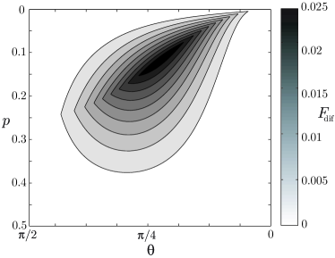
Figure 7: A contour plot of the difference, as a function of the amount of noise $p$ and the angle between the initial states $\theta$, between the average fidelities of the quantum control scheme and the best classical scheme. The quantum control scheme performs significantly better for moderate values of $p$ and $\theta$ ($0.05\lesssim p\lesssim 0.3$ and $0.3\lesssim\theta\lesssim 1$). The maximum value $F_{\mathrm{dif}}=0.026$ occurs at $p=0.115$ and $\theta=0.715$.

IV.6 Optimality

We now prove that our quantum control scheme is optimal, in that it yields the maximum average fidelity of all possible quantum operations (CPTP maps). Our proof makes use of techniques from convex optimization (specifically, those of Audenaert and Moor (2002)) but is presented without requiring any background in this subject. In the Appendix, we provide a more detailed construction of the proof.

Consider the following optimization problem: determine the maximum average fidelity

$$F_{\rm opt}=\max_{\mathcal{C}}F_{\mathcal{C}}=\max_{\mathcal{C}}\tfrac{1}{2}\sum_{i=1}^{2}{\langle\psi_{i}|\mathcal{C}\bigl{[}\mathcal{E}_{p}(|\psi_{i}\rangle\langle\psi_{i}|)\bigr{]}|\psi_{i}\rangle}\,,$$ (29)

where the maximization is now over all CPTP maps $\mathcal{C}$ acting on a single qubit.

Recall that any CPTP map $\mathcal{C}$ acting on operators on a Hilbert space $\mathcal{H}$ is in one-to-one correspondence with a density operator $\Upsilon_{\mathcal{C}}$ on $\mathcal{H}\otimes\mathcal{H}$ with

$$\mathcal{C}(\varrho)={\rm Tr_{in}}\left[(\varrho^{T}\otimes I)\Upsilon_{\mathcal{C}}\right]\,,$$ (30)

and is subject to the constraint ${\rm Tr}_{\rm out}\left[\Upsilon_{\mathcal{C}}\right]=I_{\rm in}$, where ‘in’ denotes the first subsystem and ‘out’ denotes the second Jamiolkowski (1972); D’Ariano and Presti (2001); Nielsen and Chuang (2000). With this isomorphism, the average fidelity $F_{\mathcal{C}}$ for the control scheme $\mathcal{C}$ is given by $F_{\mathcal{C}}={\rm Tr}\left[R\Upsilon_{\mathcal{C}}\right]$, where

$$R\equiv\tfrac{1}{2}\sum_{i=1}^{2}{\mathcal{E}_{p}\bigl{(}|\psi_{i}\rangle\langle\psi_{i}|\bigr{)}\otimes|\psi_{i}\langle\rangle\psi_{i}|}\,.$$ (31)

Thus, the optimization problem (29) can be rewritten as

$$\begin{array}[]{rl}\text{maximize}&{\rm Tr}\left[R\Upsilon_{\mathcal{C}}\right]\\ \text{subject to}&\Upsilon_{\mathcal{C}}\geq 0\\ &{\rm Tr}_{\rm out}\left[\Upsilon_{\mathcal{C}}\right]=I_{\rm in}\,.\end{array}$$ (32)

We now wish to prove that the maximum value of ${\rm Tr}\left[R\Upsilon_{\mathcal{C}}\right]$ subject to these constraints is given by $F_{\rm QCopt}$ of Eq. (27).

We note that, for any single-qubit operator $M$ satisfying $M\otimes I-R\geq 0$, we obtain the inequality

$${\rm Tr}\left[M\right]-{\rm Tr}\left[R\Upsilon_{\mathcal{C}}\right] ={\rm Tr}\left[(M\otimes I)\Upsilon_{\mathcal{C}}\right]-{\rm Tr}\left[R\Upsilon_{\mathcal{C}}\right]$$

$$={\rm Tr}\left[(M\otimes I-R)\Upsilon_{\mathcal{C}}\right]$$

$$\geq 0\,,$$ (33)

where the first line follows from the constraint ${\rm Tr}_{\rm out}\left[\Upsilon_{\mathcal{C}}\right]=I_{\rm in}$, and the inequality follows from the fact that $(M\otimes I-R)\geq 0$ and $\Upsilon_{\mathcal{C}}\geq 0$, and thus the trace of their product is non-negative. This inequality demonstrates that the value ${\rm Tr}\left[M\right]$ for any matrix $M$ that satisfies the constraint $(M\otimes I-R)\geq 0$ provides an upper bound on the solution of our optimization problem (32).

Consider the matrix $M=b_{0}(I+r_{x}X)$, where

$$b_{0}=\frac{1}{4}+\frac{1}{4}\sqrt{\cos^{2}{\theta}+\frac{\sin^{4}{\theta}}{1-r_{x}^{2}}}\,,$$ (34)

and $r_{x}=(1-2p)\cos\theta$ as before. It is straightforward to verify that the matrix $b_{0}I\otimes I+r_{x}b_{0}X\otimes I-R\geq 0$, and hence the value ${\rm Tr}\left[M\right]=2b_{0}$ provides an upper bound on the average fidelity of any control scheme. Because $2b_{0}$ precisely equals the fidelity of our proposed quantum control scheme, given by Eq. (27), this scheme necessarily gives an optimal solution to the original problem (32). We refer the reader to the Appendix for a more constructive proof of this result.

V Discussion and Conclusions

We have shown how two key characteristics of quantum physics – that non-orthogonal states cannot be perfectly discriminated, and that any information gain via measurement necessarily implies disturbance to the system – imply that classical strategies for control must be modified or abandoned when dealing with quantum systems. By making use of more general measurements available in quantum mechanics, we can design quantum control strategies that outperform schemes based on classical concepts. In particular, we have presented a task for which the optimal scheme relies on a non-trivial measurement strength, one that balances a tradeoff between information gain and disturbance.

In constructing our quantum control scheme for the particular task presented here, we made use of several intuitive guides. First, we used a preferred (and non-standard) ensemble of the dephasing noise operator (Eq. (15)), which allowed us to view the noise as “kicking” the state of the qubit in one direction or the other on the Bloch sphere. We then made use of a weak measurement in a basis that, loosely, attempted to acquire information about the direction of this kick without acquiring information about the choice of preparation of the system. It is remarkable (and perhaps simply lucky) that these intuitive guides lead to a quantum control scheme that was optimal for the task. It is interesting to consider whether such intuition can be applied to quantum control schemes in general, and if this intuition can be formalized into rules for developing optimal control schemes.

While our scheme is indeed optimal for the task presented, it is not guaranteed to be unique; in fact, there are other decompositions of the same CPTP map into different measurements and feedback procedures Blume-Kohout and Combes . In general, it is possible that an entire class of CPTP maps may yield the optimal performance. Also, the intuitive guides discussed above for our quantum control scheme — such as that the measurement essentially gains information only about the noise and not the choice of initial state — may not apply to other optimal schemes.

In connection to this, we note that a similar feedback control scheme was investigated by Niu and Griffiths Niu and Griffiths (1999) for optimal eavesdropping in a B92 quantum cryptography protocol Bennett (1992), see also Fuchs and Peres (1996). In their scheme, the aim of the weak measurement was to maximize the information gain about which of two non-orthogonal states was transmitted for a given amount of disturbance; in contrast, our weak measurement was designed to acquire no information about the choice of non-orthogonal states. Despite these opposing aims, the obvious similarity between these our scheme and that of Niu and Griffith warrants further investigation, particularly since we note that optimal feedback protocols exist based on different choices of measurement.

Finally, we note that the key element to our quantum control scheme — weak QND measurements on a qubit, and feedback onto a qubit based on measurement results — have both been demonstrated in recent single-photon quantum optics experiments. Specifically, Pryde et al Pryde et al. (2004) have demonstrated weak QND measurements of a single photonic qubit, and have explicitly varied the measurement strength over the full parameter range. Also, Pittman et al Pittman et al. (2005) have demonstrated feedback on the polarization of a single photon based on the measurement of the polarization of another photon entangled with the first; this feedback was used for the purposes of quantum error correction, and is essentially identical to the feedback required for our quantum control scheme. Because these core essential elements have already been demonstrated experimentally, we expect that a demonstration of our quantum control scheme is possible in the near future.

*

Appendix A Optimization Proofs

In Sec. III and IV, the proposed classical and quantum control schemes were shown to be optimal among the set of EBTP and CPTP maps, respectively. Here, we provide constructive proofs of these results in further detail.

A.1 Weak duality

Consider the following optimization:

$$\begin{array}[]{rl}\text{maximize}&{\rm Tr}\left[F_{0}Z\right]\\ \text{subject to}&Z\geq 0\\ &{\rm Tr}\left[F_{i}Z\right]=c_{i}\end{array}$$ (35)

where the matrices $F_{0}$, $F_{i}$ and the vector $c$ are specific to the problem, and $Z$ is the variable over which the optimization is performed. We say that any $Z$ satisfying the constraints of the problem is feasible. An optimization problem of this form is known as a semi-definite program (SDP), a class of convex optimization problems Boyd and Vandenberghe (2004). Each problem of the form (35) has a Lagrange dual optimization problem that arises from using the method of Lagrange multipliers and has the form Boyd and Vandenberghe (2004)

$$\begin{array}[]{rl}\text{minimize}&c^{T}x\\ \text{subject to}&-F_{0}+\sum_{i}{x_{i}F_{i}}\geq 0\end{array}$$ (36)

where now the vector $x$ is the variable to be optimized.

In many cases, such as the optimization problems investigated here, the dual problem is straightforward to solve, or else efficient numerical solutions are known that solve the primal and dual problems together. Furthermore, the dual problem allows us to bound the optimum of the original problem and this fact can be used to prove the optimality of solutions as follows.

Let $\mathfrak{d}=c^{T}x$ be the value of the objective function to be minimized in (36) for an arbitrary feasible $x$. Similarly, let $\mathfrak{p}={\rm Tr}\left[F_{0}Z\right]$ for an arbitrary feasible $Z$ and let $\mathfrak{p}^{*}$ be the optimum of our original problem (35).

We now demonstrate that, if one can find a feasible point to (35) yielding $\mathfrak{p}$ and a feasible point to (36) yielding $\mathfrak{d}$ such that $\mathfrak{d}=\mathfrak{p}$, then $\mathfrak{p}=\mathfrak{p}^{*}$, that is, the point $Z$ yielding $\mathfrak{p}$ is optimal.

Consider the difference

$$\mathfrak{d}-\mathfrak{p}=c^{T}x-{\rm Tr}\left[F_{0}Z\right]={\rm Tr}\Bigl{[}\Bigl{(}\sum_{i}{F_{i}x_{i}}-F_{0}\Bigl{)}Z\Bigr{]}\,,$$ (37)

where we have used the linearity of the trace and $c^{T}x=\sum_{i}{c_{i}x_{i}}=\sum_{i}{{\rm Tr}\left[F_{i}Zx_{i}\right]}$. As the trace is over the product of two positive semi-definite matrices, it has to be non-negative. That is to say that

$$\mathfrak{p}\leq\mathfrak{p}^{*}\leq\mathfrak{d}\,.$$ (38)

Clearly, if there is a $\mathfrak{p}$ such that $\mathfrak{p}=\mathfrak{d}$ for some $\mathfrak{d}$, then $\mathfrak{p}=\mathfrak{p}^{*}$.

A.2 Dual optimization for quantum control

As demonstrated in Sec. IV.6, obtaining the maximum average fidelity can be expressed as the optimization problem (32). For this problem (as for the classical problem which we address in the next section) the dual optimization proves to be straightforward to solve analytically and the results above can then be used to show optimality of the control scheme given by Eq. (24).

We make use of some symmetry arguments to simplify the problem. This optimization problem has certain symmetry properties under the action of the group of transformations generated by the rotation $\Upsilon\rightarrow(X\otimes X)\Upsilon(X\otimes X)^{\dagger}$ and the transpose $\Upsilon\rightarrow\Upsilon^{T}$. Specifically, the objective function is invariant under the action of this group since ${\rm Tr}[R(X\otimes X)\Upsilon(X\otimes X)]={\rm Tr}[R\Upsilon]$ and ${\rm Tr}[R\Upsilon^{T}]={\rm Tr}[R\Upsilon]$, because $(X\otimes X)R(X\otimes X)=R$ and $R^{T}=R$, respectively. In addition, the constraints are covariant under the action of the group. Since conjugation with a unitary and transposition preserve eigenvalues, $(X\otimes X)\Upsilon(X\otimes X)\geq 0$ and $\Upsilon^{T}\geq 0$ if $\Upsilon\geq 0$. To see that the equality constraints are covariant note that ${\rm Tr}_{\rm out}\left[\Upsilon_{\mathcal{C}}\right]=I_{\rm in}$ is equivalent to the condition ${\rm Tr}\left[(M\otimes I_{\rm out})\Upsilon\right]={\rm Tr}M$ for all hermitian $M$. If $\Upsilon$ obeys the partial trace constraint we have

$${\rm Tr}[(M\otimes I_{\rm out})(X\otimes X)\Upsilon(X\otimes X)]\\ ={\rm Tr}[(XMX\otimes I_{\rm out})\Upsilon]={\rm Tr}M\,,$$ (39)

and

$${\rm Tr}[(M\otimes I_{\rm out})\Upsilon^{T}]={\rm Tr}[(M^{T}\otimes I_{\rm out})\Upsilon]={\rm Tr}M\,,$$ (40)

so both $(X\otimes X)\Upsilon(X\otimes X)$ and $\Upsilon^{T}$ do also. So both the objective function and the feasible set of (32) are invariant under the action of the group. As a result there will be an invariant point $\Upsilon^{*}_{\rm inv}=(X\otimes X)\Upsilon^{*}_{\rm inv}(X\otimes X)=\Upsilon^{*T}_{\rm inv}$ that achieves the optimum $\mathfrak{p}^{*}$ Boyd and Vandenberghe (2004). We do not need to optimize over the full set of $\Upsilon$ but may restrict our attention to the set of invariant $\Upsilon_{\rm inv}$. Gatermann and Parrilo Gatermann and Parrilo (2004) have investigated such invariant SDP’s in detail.

The dual of our optimization problem (32) has the form Audenaert and Moor (2002)

$$\begin{array}[]{rl}\text{minimize}&\text{Tr}M\\ \text{subject to}&M\otimes I-R\geq 0\end{array}$$ (41)

Notice that (as is generally the case) this semidefinite program is invariant under the same group of transformations as the original problem, under which $M\rightarrow XMX$ and $M\rightarrow M^{T}$. For the dual problem we may likewise restrict attention to $M_{\rm inv}=b_{0}I+b_{x}X$ that are invariant under the action of the group. This gives a simpler dual optimization

$$\begin{array}[]{rl}\text{minimize}&2b_{0}\\ \text{subject to}&b_{0}I\otimes I+b_{x}X\otimes I-R\geq 0\,,\end{array}$$ (42)

where $b_{0}$ and $b_{x}$ are the new variables. This problem is simple enough to solve analytically; the solution is

$$b_{0}=\frac{1}{4}+\frac{1}{4}\sqrt{\cos^{2}{\theta}+\frac{\sin^{4}{\theta}}{1-r_{x}^{2}}}\,,$$ (43)

and $b_{x}=r_{x}b_{0}$ (with $r_{x}=(1-2p)\cos\theta$). This may be checked by verifying that the matrix $b_{0}I\otimes I+b_{x}X\otimes I-R$ is indeed positive semi-definite, hence $2b_{0}$ is a valid dual feasible value. Because $2b_{0}$ reproduces the fidelity of our proposed scheme, given by Eq. (27), this guess necessarily gives an optimal solution to the original problem (29).

A.3 Dual optimization for classical control

The same approach is used to solve the problem (12). We start by mapping the set of trace-preserving entanglement breaking qubit channels to bipartite states $\Upsilon_{\mathcal{B}}$. For these channels $\Upsilon_{\mathcal{B}}$ is positive, has partial trace equal to the identity, and is also separable Horodecki et al. (2003). Because $\Upsilon_{\mathcal{B}}$ is an (unnormalised) state of two qubits, the separability condition is equivalent to the positivity of the partial transpose Horodecki et al. (1996). We will denote the partial transpose of the operator $\Upsilon_{\mathcal{B}}$ on the subsystem $\mathcal{H}_{\rm out}$ by $\Upsilon_{\mathcal{B}}^{T_{\rm out}}$ . Thus we may rephrase the optimization problem (12) in the form

$$\begin{array}[]{rl}\text{maximize}&{\rm Tr}\left[R\Upsilon_{\mathcal{B}}\right]\\ \text{subject to}&\Upsilon_{\mathcal{B}}\geq 0\,,\quad\Upsilon_{\mathcal{B}}^{T_{\rm out}}\geq 0\\ &{\rm Tr}_{\rm out}\Upsilon_{\mathcal{B}}=I_{\rm in}.\end{array}$$ (44)

Note that the condition of positivity of the partial transpose guarantees that $\Upsilon_{\mathcal{B}}$ corresponds to an EBTP map.

The new problem has the same symmetries as the full optimization (32) with one addition. Notice that $R^{T_{out}}=R$ so the objective function of both problems is invariant under partial transpose. In our new problem the point $\Upsilon_{\mathcal{B}}^{T_{\rm out}}$ is feasible if $\Upsilon_{\mathcal{B}}$ is feasible, so the feasible set is also invariant under the partial transpose. (Note that since partial transpose does not preserve positivity this is not true of the problem (32)). Because of this symmetry we may restrict our attention to $\Upsilon_{\rm inv}$ for which $\Upsilon^{T_{\rm out}}_{\rm inv}=\Upsilon_{\rm inv}$. Since the partial transpose sends $A\otimes Y\rightarrow-A\otimes Y$ where $A$ is any Hermitian matrix, we can conclude that ${\rm Tr}[(A\otimes Y)\Upsilon_{\rm inv}]=0$. It is sufficient to check this condition for the full set of Pauli matrices $I,X,Y,Z$ so the requirement of invariance under the partial transpose constitutes four new constraints. Notice however that the condition $\Upsilon^{T_{\rm out}}_{\rm inv}\geq 0$ is now redundant since we are requiring that $\Upsilon^{T_{\rm out}}_{\rm inv}=\Upsilon^{T_{\rm inv}}$. So we can replace the problem (44) with

$$\begin{array}[]{rl}\text{maximize}&{\rm Tr}\left[R\Upsilon_{\mathcal{B}}\right]\\ \text{subject to}&\Upsilon_{\mathcal{B}}\geq 0\\ &{\rm Tr}_{\rm out}\Upsilon_{\mathcal{B}}=I_{\rm in}\\ &{\rm Tr}(A\otimes Y)\Upsilon_{\mathcal{B}}=0\quad\forall A\in\{I,X,Y,Z\}.\end{array}$$ (45)

Positivity of the partial transpose and hence the separability of $\Upsilon_{\mathcal{B}}$ is now guaranteed by the positivity of $\Upsilon_{\mathcal{B}}$ and the additional equality constraints.

The dual of the problem (45) is

$$\begin{array}[]{rl}\text{minimize}&\text{Tr}M\\ \text{subject to}&I\otimes M+N\otimes Y-R\geq 0\end{array}$$ (46)

This semidefinite program still has symmetries corresponding to the rotation $X\otimes X$ and the transpose (but not under the partial transpose.) These two symmetries lead to the transformations $N\rightarrow-XNX$ and $N\rightarrow-N^{T}$ respectively. The only invariant choices of $N$ are proportional to $Y$. As before we may restrict attention to $M_{\rm inv}=a_{0}I+a_{x}X$ that are invariant under the action of the group and $N_{\rm inv}=a_{y}Y$. This gives a simpler dual optimization

$$\begin{array}[]{rl}\text{minimize}&2a_{0}\\ \text{subject to}&a_{0}I\otimes I+a_{x}X\otimes I+a_{y}Y\otimes Y-R\geq 0\,,\end{array}$$ (47)

where $a_{0},a_{x}$ and $a_{y}$ are the new variables. This problem should be compared to the analogous dual optimization in the quantum case (42). Again, this problem can be solved analytically, yielding the solution

$$a_{0} =\frac{1}{4}+\frac{1}{4}\sqrt{\cos^{2}{\theta}+\sin^{4}{\theta}}\,,$$ (48)

$$a_{x} =\frac{r_{x}}{4}+\frac{r_{x}}{4}\frac{\cos^{2}{\theta}}{\sqrt{\cos^{2}{\theta}+\sin^{4}{\theta}}}\,,$$ (49)

$$a_{y} =-\frac{r_{x}}{4}\frac{\cos{\theta}\sin^{2}{\theta}}{\sqrt{\cos^{2}{\theta}+\sin^{4}{\theta}}}\,.$$ (50)

Again, one can check that $a_{0}I\otimes I+a_{x}X\otimes I+a_{y}Y\otimes Y-R$ is positive semidefinite with these choices, which ensures that the objective function $2a_{0}$ is indeed a dual feasible value. The proof of optimality follows as before in the quantum case by: (i) observing that $2a_{0}$ reproduces the fidelity $F_{\rm DR2}$ of Eq. (11) and (ii) applying the weak duality argument.

We note that the optimization techniques presented here may be useful when applied to more general problems presented in Fuchs and Sasaki Fuchs and Sasaki (2003). However, when the map in question does not act on qubits, there are significant complications in characterizing the EBTP maps because the PPT condition is no longer sufficient.

References

- Belavkin (1983) V. P. Belavkin, Autom. Remote Control 44, 178 (1983), quant-ph/0408003.
- Belavkin (1999) V. P. Belavkin, Rep. Math. Phys. 45, 353 (1999).
- Armen et al. (2002) M. A. Armen, J. K. Au, J. K. Stockton, A. C. Doherty, and H. Mabuchi, Phys. Rev. Lett. 89, 133602 (2002).
- Smith et al. (2002) W. P. Smith, J. E. Reiner, L. A. Orozco, S. Kuhr, and H. M. Wiseman, Phys. Rev. Lett. 89, 133601 (2002).
- Geremia et al. (2004) J. Geremia, J. K. Stockton, and H. Mabuchi, Science 304, 270 (2004).
- Reiner et al. (2004) J. E. Reiner, W. P. Smith, L. A. Orozco, H. M. Wiseman, and J. Gambetta, Phys. Rev. A 70, 023819 (2004).
- LaHaye et al. (2004) M. D. LaHaye, O. Buu, B. Camarota, and K. C. Schwab, Science 304, 74 (2004).
- Bushev et al. (2006) P. Bushev, D. Rotter, A. Wilson, F. Dubin, C. Becher, J. Eschner, R. Blatt, V. Steixner, P. Rabl, and P. Zoller, Phys. Rev. Lett. 96, 043003 (2006).
- 05j (2005) Special issue on quantum control, J. Opt B, 7, no. 10 (2005).
- Wiseman et al. (2002) H. M. Wiseman, S. Mancini, and J. Wang, Phys. Rev. A 66, 013807 (2002).
- Wang and Wiseman (2001) J. Wang and H. M. Wiseman, Physical Review A 64, 063810 (2001).
- Lidar and Schneider (2005) D. A. Lidar and S. Schneider, Quant. Info. Comp. 5, 350 (2005).
- van Handel et al. (2005) R. van Handel, J. K. Stockton, and H. Mabuchi, IEEE Trans. Automat. Control 50, 768 (2005).
- (14) M. Mirrahimi and R. van Handel, math-ph/05100066.
- Gregoratti and Werner (2003) M. Gregoratti and R. F. Werner, J. Mod. Opt 50, 915 (2003).
- Gregoratti and Werner (2004) M. Gregoratti and R. F. Werner, J. Math. Phys. 45, 2600 (2004).
- Doherty et al. (2001) A. C. Doherty, K. Jacobs, and G. Jungman, Phys. Rev. A 63, 062306 (2001).
- Niu and Griffiths (1999) C.-S. Niu and R. B. Griffiths, Phys. Rev. A 60, 2764 (1999).
- Lloyd and Viola (2001) S. Lloyd and L. Viola, Phys. Rev. A 65, 010101 (2001).
- Nielsen and Chuang (2000) M. A. Nielsen and I. L. Chuang, Quantum Computation and Quantum Information (Cambridge University Press, Cambridge, 2000).
- Preskill (2000) J. Preskill, quant-ph/0010098.
- Horodecki et al. (2003) M. Horodecki, P. W. Shor, and M. B. Ruskai, Rev. Math. Phys. 15, 629 (2003), quant-ph/0302031.
- Ruskai (2003) M. B. Ruskai, Rev. Math. Phys. 15, 643 (2003), quant-ph/0302032.
- Holevo (1998) A. S. Holevo, quant-ph/9809023.
- Helstrom (1976) C. W. Helstrom, Quantum Detection and Estimation Theory, vol. 123 of Mathematics in Science and Engineering (Academic Press, New York, 1976).
- Fuchs and Sasaki (2003) C. A. Fuchs and M. Sasaki, Quantum Info. Comp. 3, 377 (2003).
- Fuchs and Peres (1996) C. A. Fuchs and A. Peres, Phys. Rev. A 53, 2038 (1996).
- Pryde et al. (2004) G. J. Pryde, J. L. O’Brien, A. G. White, S. D. Bartlett, and T. C. Ralph, Phys. Rev. Lett. 92, 190402 (2004).
- Ralph et al. (2006) T. C. Ralph, S. D. Bartlett, J. L. O’Brien, G. J. Pryde, and H. M. Wiseman, Phys. Rev. A 73, 012113 (2006).
- Audenaert and Moor (2002) K. Audenaert and B. D. Moor, Phys. Rev. A 65, 030302 (2002).
- Jamiolkowski (1972) A. Jamiolkowski, Rep. Math. Phys. 3, 275 (1972).
- D’Ariano and Presti (2001) G. M. D’Ariano and P. L. Presti, Phys. Rev. A 64, 042308 (2001).
- (33) R. Blume-Kohout and J. Combes, private communication.
- Bennett (1992) C. H. Bennett, Phys. Rev. Lett. 68, 3121 (1992).
- Pittman et al. (2005) T. B. Pittman, B. C. Jacobs, and J. D. Franson, Phys. Rev. A 71, 052332 (2005).
- Boyd and Vandenberghe (2004) S. Boyd and L. Vandenberghe, Convex Optimization (Cambridge University Press, 2004).
- Gatermann and Parrilo (2004) K. Gatermann and P. A. Parrilo, Journal of Pure and Appl. Algebra 192, 95 (2004), math.AC/0211450.
- Horodecki et al. (1996) M. Horodecki, P. Horodecki, and R. Horodecki, Phys. Lett. A 223, 1 (1996).