Statistical analysis on testing of an entangled state
based on Poisson distribution framework

Abstract

A hypothesis testing scheme for entanglement has been formulated based on the Poisson distribution framework instead of the POVM framework. Three designs were proposed to test the entangled states in this framework. The designs were evaluated in terms of the asymptotic variance. It has been shown that the optimal time allocation between the coincidence and anti-coincidence measurement bases improves the conventional testing method. The test can be further improved by optimizing the time allocation between the anti-coincidence bases.

I Introduction

Entangled states are an essential resource for various quantum information processingsBennett93 ; Briegel98 . Hence, it is required to generate maximally entangled states. However, for a practical use, it is more essential to guarantee the quality of generated entangled states. Statistical hypothesis testing is a standard method for guaranteeing the quality of industrial products. Therefore, it is much needed to establish the method for statistical testing of maximally entangled states.

Quantum state estimation and quantum state tomography are known as the method of identifying the unknown stateSelected ; helstrom ; holevo . Quantum state tomography WJEK99 has been recently applied to obtain full information of the $4\times 4$ density matrix. However, if the purpose is testing of entanglement, it is more economical to concentrate on checking the degree of entanglement. Such a study has been done by Tsuda et al TMH05 as optimization problems of POVM. However, an implemented quantum measurement cannot be regarded as an application of a POVM to a single particle system or a multiple application of a POVM to single particle systems. In particular, in quantum optics, the following measurement is often realized, which is not described by a POVM on a single particle system. The number of generated particles is probabilistic. We prepare a filter corresponding to a projection $P$, and detect the number of particle passing through the filter. If the number of generated particles obeys a Poisson distribution, as is mentioned in Section II, the number of detected particles obeys another Poisson distribution whose average is given by the density and the projection $P$.

In this kind of measurements, if any particle is not detected, we cannot decide whether a particle is not generated or it is generated but does not pass through the filter. If we can detect the number of generated particles as well as the number of passing particles, the measurement can be regarded as the multiple application of the POVM $\{P,I-P\}$. In this case, the number of applications of the POVM is the variable corresponding to the number of generated particles. Also, we only can detect the empirical distribution. Hence, our obtained information almost discuss by use of the POVM $\{P,I-P\}$.

However, if it is impossible to distinguish the two events by some imperfections, it is impossible to reduce the analysis of our obtained information to the analysis of POVMs. Hence, it is needed to analyze the performance of the estimation and/or the hypothesis testing based on the Poisson distribution describing the number of detected particles. If we discuss the ultimate bound of the accuracy of the estimation and/or the hypothesis testing, we do not have to treat such imperfect measurements. Since several realistic measurements have such imperfections, it is very important to optimize our measurement among such a class of imperfect measurements.

In this paper, our measurement is restricted to the detection of the number of the particle passing through the filter corresponding to a projection $P$. We apply this formulation to the testing of maximally entangled states on two qubit systems (two-level systems), each of which is spanned by two vectors $|H\rangle$ and $|V\rangle$. Since the target system is a bipartite system, it is natural to restrict to our measurement to local operations and classical communications (LOCC). In this paper, for a simple realization, we restrict our measurements to the number of the simultaneous detections at the both parties of the particles passing through the respective filters. We also restrict the total measurement time $t$, and optimize the allocation of the time for each filters at the both parties.

As our results, we obtain the following characterizations. If the average number of the generated particles is known, our choice is counting the coincidence events or the anti-coincidence events. When the true state is close to the target maximally entangled state $|\Phi^{(+)}\rangle:=\frac{1}{\sqrt{2}}(|HH\rangle+|VV\rangle)$ (that is, the fidelity between these is greater than $1/4$), the detection of anti-coincidence events is better than that of coincidence events. This result implies that the indistinguishability between the coincidence events and the non-generation event loses less information than that between the anti-coincidence events and the non-generation event.

This fact also holds even if we treat this problem taking into account the effect of dark counts. In this discussion, in order to remove the bias concerning the direction of the difference, we assume the equal time allocation among the vectors $\{|HV\rangle,|VH\rangle,|DX\rangle,|XD\rangle,|RR\rangle,|LL\rangle\}$, which corresponds to the anti-coincidence events, and that among the vectors $\{|HH\rangle,|VV\rangle,|DD\rangle,|XX\rangle,|RL\rangle,|LR\rangle\}$, which corresponds to the coincidence events, where $|D\rangle:=\frac{1}{2}(|H\rangle+|V\rangle)$, $|X\rangle:=\frac{1}{2}(|H\rangle-|V\rangle)$, $|R\rangle:=\frac{1}{2}(|H\rangle+i|V\rangle)$, $|L\rangle:=\frac{1}{2}(|H\rangle-i|V\rangle)$. Indeed, Barbieri et al BMNMDM03 proposed to detect the anti-coincidence events for measuring an entanglement witness, they did not prove the superiority of detecting the anti-coincidence events in the framework of mathematical statistics.

However, the average number of the generated particles is usually unknown. In this case, we cannot estimate how close the true state is to the target maximally entangled state from the detection of anti-coincidence events. Hence, we need to count the coincidence events as additional information. in order to resolve this problem, we usually use the equal allocation between anti-coincidence events and coincidence events in the visibility method, which is a conventional method for checking the entanglement. However, since we measure the coincidence events and the anti-coincidence events based on one or two bases in this method, there is a bias concerning the direction of the difference. In order to remove this bias, we consider the detecting method with the equal time allocation among all vectors $\{|HV\rangle,|VH\rangle,|DX\rangle,|XD\rangle,|RR\rangle,|LL\rangle\}$ and $\{|HH\rangle,|VV\rangle,|DD\rangle,|XX\rangle,|RL\rangle,|LR\rangle\}$, and call it the modified visibility method.

In this paper, we also examine the detection of the total flux, which can be realized by detecting the particle without the filter. We optimize the time allocation among these three detections. We found that the optimal time allocation depends on the fidelity between the true state and the target maximally entangled state. If our purpose is estimating the fidelity $F$, we cannot directly apply the optimal time allocation. However, the purpose is testing whether the fidelity $F$ is greater than the given threshold $F_{0}$, the optimal allocation at $F_{0}$ gives the optimal testing method.

If the fidelity $F$ is less than a critical value, the optimal allocation is given by the allocation between the anti-coincidence vectors and the coincidence vectors (the ratio depends on $F$.) Otherwise, it is given by the allocation only between the anti-coincidence vectors and the total flux. This fact is valid even if the dark count exists. If the dark count is greater than a certain value, the optimal time allocation is always given by the allocation between the anti-coincidence vectors and the coincidence vectors.

Further, we consider the optimal allocation among anti-coincidence vectors when the average number of generated particles. The optimal allocation depends on the direction of the difference between the true state and the target state. Since the direction is usually unknown, this optimal allocation dose not seems useful. However, by adaptively deciding the optimal time allocation, we can apply the optimal time allocation. We propose to apply this optimal allocation by use of the two-stage method. Further, taking into account the complexity of testing methods and the dark counts, we give a testing procedure of entanglement based on the two-stage method. In addition, proposed designs of experiments were demonstrated by Hayashi et al. HSTMTJ in two photon pairs generated by spontaneous parametric down conversion (SPDC).

In this article, we reformulate the hypothesis testing to be applicable to the Poisson distribution framework, and demonstrate the effectiveness of the optimized time allocation in the entanglement test. The construction of this article is following. Section II defines the Poisson distribution framework and gives the hypothesis scheme for the entanglement. Section III gives the mathematical formulation concerning statistical hypothesis testing. Sections IV and V give the fundamental properties of the hypothesis testing: section IV introduces the likelihood ratio test and its modification, and section V gives the asymptotic theory of the hypothesis testing. Sections VI-IX are devoted to the designs of the time allocation between the coincidence and anti-coincidence bases: section VI defines the modified visibility method, section VII optimize the time allocation, when the total photon flux $\lambda$ is unknown, section VIII gives the results with known $\lambda$, and section IX compares the designs in terms of the asymptotic variance. Section X gives further improvement by optimizing the time allocation between the anti-coincidence bases. Appendices give the detail of the proofs used in the optimization.

II Hypothesis Testing scheme for entanglement in Poisson distribution framework

Let ${\cal H}$ be the Hilbert space of our interest, and $P$ be the projection corresponding to our filter. If we assume generation process on each time to be identical but individual, the total number $n$ of generated particles during the time $t$ obeys the Poisson distribution ${\rm Poi}(\lambda t)(n):=e^{-\lambda t}\frac{(\lambda t)^{n}}{n!}$. Hence, when the density of the true state is $\sigma$, the probability of the number $k$ of detected particles is given as

$$\sum_{n=0}^{\infty}{\rm Poi}(\lambda t)(n)\genfrac{(}{)}{0.0pt}{}{n}{k}(\mathop{\mathbf{Tr}}\nolimits P\sigma)^{k}(1-\mathop{\mathbf{Tr}}\nolimits P\sigma)^{n-k}$$

$$= {\rm Poi}(\lambda t\mathop{\mathbf{Tr}}\nolimits P\sigma)(k).$$ (1)

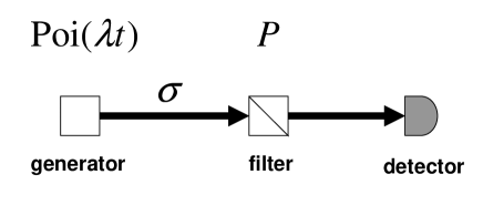
Figure 1: Experimental scheme in Poisson distribution framework

In fact, if we treat the Fock space generated by ${\cal H}$ instead of the single particle system ${\cal H}$, this measurement can be described by a POVM. However, since this POVM dooes not have a simple form, it is suitable to treat this measurement in the form (1).

Further, if we errorly detect the $k^{\prime}$ particles with the probability ${\rm Poi}(\delta t)(k^{\prime})$, the probability of the number $k$ of detected particles is equal to

$$\sum_{k^{\prime}=0}^{k}{\rm Poi}(\lambda t\mathop{\mathbf{Tr}}\nolimits P\sigma)(k-k^{\prime})+{\rm Poi}(\delta t)(k^{\prime})$$

$$= {\rm Poi}((\lambda\mathop{\mathbf{Tr}}\nolimits P\sigma+\delta)t)(k).$$

This kind of incorrect detection is called dark count. Further, since we consider the bipartite case, i.e., the case where ${\cal H}=\mathbb{C}^{2}\otimes\mathbb{C}^{2}$, we assume that our projection $P$ has the separable form $P_{1}\otimes P_{2}$.

In this paper, under the above assumption, we discuss the hypothesis testing when the target state is the maximally entangled $|\Phi^{(+)}\rangle$ state while Usami et al.Usami discussed the state estimation under this assumption. Here we measure the degree of entanglement by the fidelity between the generated state and the target state:

$$F=\langle\Phi^{(+)}|\sigma|\Phi^{(+)}\rangle.$$ (2)

The purpose of the test is to guarantee that the state is sufficiently close to the maximally entangled state with a certain significance. That is, we are required to disprove that the fidelity $F$ is less than a threshold $F_{0}$ with a small error probability. In mathematical statistics, this situation is formulated as hypothesis testing; we introduce the null hypothesis $H_{0}$ that entanglement is not enough and the alternative $H_{1}$ that the entanglement is enough:

$$H_{0}:F\leq F_{0}\hbox{ v.s. }H_{1}:F>F_{0},$$ (3)

with a threshold $F_{0}$.

Visibility is an indicator of entanglement commonly used in the experiments, and is calculated as follows: first, A’s measurement vector $|x_{A}\rangle$ is fixed, then the measurement $|x_{A},y_{B}\rangle$ is performed by rotating B’s measurement vector $|x_{B}\rangle$ to obtain the maximum and minimum number of the counts, $n_{max}$ and $n_{min}$. We need to make the measurement with at least two bases of A in order to exclude the possibility of the classical correlation. We may choose the two bases $\{|H\rangle,|V\rangle\}$ and $\{|D\rangle,|X\rangle\}$ as $|x_{A}\rangle$, for example. Finally, the visibility is given by the ratio between $n_{max}-n_{min}$ and $n_{max}+n_{min}$ with the respective A’s measurement basis $|x_{A}\rangle$. However, our decision will contain a bias, if we choose only two bases as A’s measurement basis $|x_{A}\rangle$. Hence, we cannot estimate the fidelity between the target maximally entangled state and the given state in a statistically proper way from the visibility.

Since the equation

$$|HH\rangle\langle HH|+|VV\rangle\langle VV|+|DD\rangle\langle DD|$$

$$+|XX\rangle\langle XX|+|RL\rangle\langle RL|+|LR\rangle\langle LR|$$

$$= 2|\Phi^{(+)}\rangle\langle\Phi^{(+)}|+I$$ (4)

holds, we can estimate the fidelity by measuring the sum of the counts of the following vectors: $|HH\rangle,|VV\rangle,|DD\rangle,|XX\rangle,|RL\rangle,$ and $|LR\rangle$, when $\lambda$ is knownBMNMDM03 ; TMH05 . This is because the sum $n_{1}:=n_{HH}+n_{VV}+n_{DD}+n_{XX}+n_{RL}+n_{LR}$ obeys the Poisson distribution with the expectation value $(\lambda\frac{1+2F}{6}+\delta)t_{1}$, where the measurement time for each vector is $\frac{t_{1}}{6}$. We call these vectors the coincidence vectors because these correspond to the coincidence events.

However, since the parameter $\lambda$ is usually unknown, we need to perform another measurement on different vectors to obtain additional information. Since

$$|HV\rangle\langle HV|+|VH\rangle\langle VH|+|XD\rangle\langle XD|$$

$$+|DX\rangle\langle DX|+|RR\rangle\langle RR|+|LL\rangle\langle LL|$$

$$= 2I-2|\Phi^{(+)}\rangle\langle\Phi^{(+)}|$$ (5)

also holds, we can estimate the fidelity by measuring the sum of the counts of the following vectors: $|HV\rangle,|VH\rangle,|DX\rangle,|XD\rangle,|RR\rangle$, and $|LL\rangle$. The sum $n_{2}:=n_{HV}+n_{VH}+n_{DX}+n_{XD}+n_{RR}+n_{LL}$ obeys the Poisson distribution $\rm Poi((\lambda\frac{2-2F}{6}+\delta)t_{2})$, where the measurement time for each vector is $\frac{t_{2}}{6}$. Combining the two measurements, we can estimate the fidelity without the knowledge of $\lambda$. We call these vectors the anti-coincidence vectors because these correspond to the anti-coincidence events.

We can also consider different type of measurement on $\lambda$. If we prepare our device to detect all photons, i.e., the case where the projection is $I\otimes I$, the detected number $n_{3}$ obeys the distribution $\rm Poi((\lambda+\delta)t_{3}$) with the measurement time $t_{3}$. We will refer to it as the total flux measurement. In the following, we consider the best time allocation for estimation and test on the fidelity, by applying methods of mathematical statistics. We will assume that $\lambda$ is known or estimated from the detected number $n_{3}$.

III Hypothesis testing for probability distributions

III.1 Formulation

In this section, we review the fundamental knowledge of hypothesis testing for probability distributionslehmann . Suppose that a random variable $X$ is distributed according to a probability measure $P_{\theta}$ identified by the unknown parameter $\theta$. We also assume that the unknown parameter $\theta$ belongs to one of mutually disjoint sets $\Theta_{0}$ and $\Theta_{1}$. When we want to guarantee that the true parameter $\theta$ belongs to the set $\Theta_{1}$ with a certain significance, we choose the null hypothesis $H_{0}$ and the alternative hypothesis $H_{1}$ as

$$H_{0}:\theta\in\Theta_{0}\mbox{ versus }H_{1}:\theta\in\Theta_{1}.$$ (6)

Then, our decision method is described by a test, which is described as a function $\phi(x)$ taking values in $\{0,1\}$; $H_{0}$ is rejected if $1$ is observed, and $H_{0}$ is not rejected if $0$ is observed. That is, we make our decision only when $1$ is observed, and do not otherwise. This is because the purpose is accepting $H_{1}$ by rejecting $H_{0}$ with guaranteeing the quality of our decision, and is not rejecting $H_{1}$ nor accepting $H_{1}$. Therefore, we call the region $\{x|\phi(1)=1\}$ the rejection region. The test $\phi$ can be defined by the rejection region. In fact, we choosed the hypothesis that the fidelity is less than the given threshold $\theta_{0}$ as the null hypothesis $H_{0}$ in Section II. This formulation is natural because our purpose is guaranteeing that the fidelity is not less than the given threshold $\theta_{0}$.

From theoretical viewpoint, we often consider randomized tests, in which we probabilistically make the decision for a given data. Such a test is given by a function $\phi$ mapping to the interval $[0,1]$. When we observe the data $x$, $H_{0}$ is rejected with the probability $\phi(x)$. In the following, we treat randomized tests as well as deterministic tests.

In the statistical hypothesis testing, we minimize error probabilities of the test $\phi$. There are two types of errors. The type one error is the case where $H_{0}$ is rejected though it is true. The type two error is the converse case, $H_{0}$ is accepted though it is false. Hence, the type one error probability is given $P_{\theta}(\phi)$ $(\theta\in\Theta_{0})$, and the type two error probability is given $1-P_{\theta^{\prime}}(\phi)$ $(\theta^{\prime}\in\Theta_{1})$, where

$$P_{\theta}(\phi)=\int\phi(x)dP_{\theta}(x).$$

It is in general impossible to minimize both $P_{\theta}(\phi)$ and $1-P_{\theta^{\prime}}(\phi)$ simultaneously because of a trade-off relation between them. Since we make our decision with guaranteeing its quality only when $1$ is observed, it is definitively required that the type one error probability $P_{\theta}(\phi)$ is less than a certain constant $\alpha$. For this reason, we minimize the type two error probability $1-P_{\theta^{\prime}}(\phi)$ under the condition $P_{\theta}(\phi)\leq\alpha$. The constant $\alpha$ in the condition is called the risk probability, which guarantees the quality of our decision. If the risk probability is large enough, our decision has less reliability. Under this constraint for the risk probability, we maximize the probability to reject the hypothesis $H_{0}$ when the true parameter is $\theta^{\prime}\in\Theta_{1}$. This probability is given as $P_{\theta}(\phi)$, and is called the power of $\phi$. Hence, a test $\phi$ of the risk probability $\alpha$ is said to be most powerful (MP) at $\theta^{\prime}\in\Theta_{1}$ if $P_{\theta^{\prime}}(\phi)\geq P_{\theta^{\prime}}(\psi)$ holds for any test $\psi$ of the risk probability $\alpha$. Then, a test is said to be Uniformly Most Powerful (UMP) if it is MP at any $\theta^{\prime}\in\Theta_{1}$.

III.2 p-values

In the hypothesis testing, we usually fixed our test before applying it to data. However, we sometimes focus on the minimum risk probability among tests in a class $\tilde{T}$ rejecting the hypothesis $H_{0}$ with a given data. This value is called the p-value, which depends on the observed data $x$ as well as the subset $\Theta_{0}$ to be rejected.

In fact, in order to define the p-value, we have to fix a class $T$ of tests. Then, for $x$ and $\Theta_{0}$, p-value is defined as

$$\min_{\phi\in T:\phi(x)=1}\max_{\theta\in\Theta_{0}}P_{\theta}(\phi).$$ (7)

Since the p-value expresses the risk for rejecting the hypothesis $H_{0}$, Hence, this concept is useful for comparison among several designs of experiment.

Note that if we are allowed to choose any function $\phi$ as a test, the above minimum is attained by the function $\delta_{x}$:

$$\delta_{x}(y)=\left\{\begin{array}[]{ll}0&\hbox{ if }y\neq x\\ 1&\hbox{ if }y=x.\end{array}\right.$$ (10)

In this case, the p-vale is $\max_{\theta\in\Theta_{0}}P_{\theta}(x)$. However, the function $\delta_{x}$ is unnatural as a test. Hence, we should fix a class of tests to define p-value.

IV Likelihood Test

IV.1 Definition

In mathematical statistics, the likelihood ratio tests is often used as a class of standard testslehmann . This kind of tests often provide the UMP test in some typical cases. When both $\Theta_{0}$ and $\Theta_{1}$ consist of single elements as $\Theta_{0}=\{\theta_{0}\}$ and $\Theta_{1}=\{\theta_{1}\}$, the likelihood ratio test $\phi_{\mathop{\rm LR}\nolimits,r}$ is defined as

$$\phi_{\mathop{\rm LR}\nolimits,r}(x):=\begin{cases}0&{\rm if}\ P_{\theta_{0}}(x)/P_{\theta_{1}}(x)\geq r,\cr 1&{\rm if}\ P_{\theta_{0}}(x)/P_{\theta_{1}}(x)<r\end{cases}$$

where $r$ is a constant, and the ratio $P_{\theta_{0}}(x)/P_{\theta_{1}}(x)$ is called the likelihood ratio. From the definition, any test $\phi$ satisfies

$$(rP_{\theta_{1}}-P_{\theta_{0}})(\phi_{\mathop{\rm LR}\nolimits,r})\geq(rP_{\theta_{1}}-P_{\theta_{0}})(\phi).$$ (11)

When a likelihood ratio test $\phi_{\mathop{\rm LR}\nolimits,r}$ satisfies

$$\alpha=P_{\theta_{0}}(\phi_{\mathop{\rm LR}\nolimits,r}),$$ (12)

the test $\phi_{\mathop{\rm LR}\nolimits,r}$ is MP of level $\alpha$. Indeed, when a test $\phi$ satisfies $P_{\theta_{0}}(\phi)\leq\alpha$,

$$-\alpha+rP_{\theta_{1}}(\phi)=-P_{\theta_{0}}(\phi)+rP_{\theta_{1}}(\phi)$$

$$\leq -P_{\theta_{0}}(\phi_{\mathop{\rm LR}\nolimits,r})+rP_{\theta_{1}}(\phi_{\mathop{\rm LR}\nolimits,r})=-\alpha+rP_{\theta_{1}}(\phi_{\mathop{\rm LR}\nolimits,r}).$$

Hence, $1-P_{\theta_{1}}(\phi)\geq 1-P_{\theta_{1}}(\phi_{\mathop{\rm LR}\nolimits,r})$. This is known as Neyman-Pearson’s fundamental lemma.

The likelihood ratio test is generalized to the cases where $\Theta_{0}$ or $\Theta_{1}$ has at least two elements as

$$\phi_{\mathop{\rm LR}\nolimits,r}(x):=\begin{cases}0&{\rm if}\ \frac{\sup_{\theta\in\Theta_{0}}P_{\theta}(x)}{\sup_{\theta\in\Theta_{1}}P_{\theta}(x)}\geq r,\cr 1&{\rm if}\ \frac{\sup_{\theta\in\Theta_{0}}P_{\theta}(x)}{\sup_{\theta\in\Theta_{1}}P_{\theta}(x)}<r.\end{cases}$$

Usually, in order to guarantee a small risk probability, the likelihood ratio $r$ is choosed as $r<1$.

IV.2 Monotone Likelihood Ratio Test

In cases where the hypothesis is one-sided, that is, the parameter space $\Theta$ is an interval of $\mathbb{R}$ and the hypothesis is given as

$$H_{0}:\theta\geq\,\theta_{0}\mbox{ versus }H_{1}:\theta<\,\theta_{0},$$ (13)

we often use so-called interval tests for its optimality under some conditions as well as for its naturalness.

When the likelihood ratio $P_{\theta}(x)/P_{\eta}(x)$ is monotone increasing concerning $x$ for any $\theta,\eta$ such that $\theta>\eta$, the likelihood ratio is called monotone. In this case, the likelihood ratio test $\phi_{\mathop{\rm LR}\nolimits,r}$ between $P_{\theta_{0}}$ and $P_{\theta_{1}}$ is UMP of level $\alpha:=P_{\theta_{0}}(\phi_{\mathop{\rm LR}\nolimits,r})$, where $\theta_{1}$ is an arbitrary element satisfying $\theta_{1}<\theta_{0}$.

Indeed, many important examples satisfy this condition. Hence, it is convenient to give its proof here.

From the monotonicity, the likelihood ratio test $\phi_{\mathop{\rm LR}\nolimits,r}$ has the form

$$\phi_{\mathop{\rm LR}\nolimits,r}(x)=\left\{\begin{array}[]{ll}1&x<x_{0}\\ 0&x\geq x_{0}\end{array}\right.$$ (16)

with a threshold value $x_{0}$. Since the monotonicity implies $P_{\theta_{0}}(\phi_{\mathop{\rm LR}\nolimits,r})\geq P_{\theta}(\phi_{\mathop{\rm LR}\nolimits,r})$ for any $\theta\in\Theta_{0}$, it follows from Neyman Pearson Lemma that the likelihood ratio test $\phi_{\mathop{\rm LR}\nolimits,r}$ is MP of level $\alpha$. From (16), the likelihood ratio test $\phi_{\mathop{\rm LR}\nolimits,r}$ is also a likelihood ratio test between $P_{\theta_{0}}$ and $P_{\eta}$, where $\eta$ is another element satisfying $\eta<\theta_{0}$. Hence, the test $\phi_{\mathop{\rm LR}\nolimits,r}$ is also MP of level $\alpha$.

From the above discussion, it is suitable to treat p-value based on the class of likelihood ratio tests. In this case, when we observe $x_{0}$, the p-value is equal to

$$\int_{-\infty}^{x_{0}}P_{\theta_{0}}(dx).$$ (17)

IV.3 One-Parameter Exponential Family

In mathematical statistics, exponential families are known as a class of typical statistical modelsA-N . A family of probability distributions $\{P_{\theta}|\theta\subset\Theta\}$ is called an exponential family when there exists a random variable $x$ such that

$$P_{\theta}(x):=P_{0}(x)\exp(\theta x+g(\theta)),$$ (18)

where $g(\theta):=-\log\int\exp(\theta x)P_{0}(dx)$.

It is known that this class of families includes, for example, the Poisson distributions, normal distributions, binomial distributions, etc. In this case, the likelihood ratio $\frac{\exp(\theta_{0}x+g(\theta_{0}))}{\exp(\theta_{1}x+g(\theta_{1}))}=\exp((\theta_{0}-\theta_{1})x+g(\theta_{0})-g(\theta_{1}))$ is monotone concerning $x$ for $\theta_{0}>\theta_{1}$. Hence, the likelihood ratio test is UMP in the hypothesis (13). Note that this argument is valid even if we choose a different parameter if the family has a parameter satisfying (18).

For example, in the case of the normal distribution $P_{\theta}(x)=\frac{1}{\sqrt{2\pi V}}e^{-\frac{(x-\theta)^{2}}{2V}}=\frac{1}{\sqrt{2\pi V}}e^{-\frac{x^{2}}{2V}+\frac{\theta x}{V}-\frac{\theta^{2}}{2V}}$, the UMP test $\phi_{\mathop{\rm UMP}\nolimits,\alpha}$ of the level $\alpha$ is given as

$$\phi_{\mathop{\rm UMP}\nolimits,\alpha}(x):=\left\{\begin{array}[]{ll}1&\hbox{ if }x<\theta_{0}-\epsilon_{\alpha}\sqrt{V}\\ 0&\hbox{ if }x\geq\theta_{0}-\epsilon_{\alpha}\sqrt{V},\end{array}\right.$$ (21)

where

$$\Phi(-\epsilon_{\alpha})=\alpha,\quad\Phi(\epsilon)=\int^{\epsilon}_{-\infty}\frac{1}{\sqrt{2\pi}}e^{-\frac{x^{2}}{2}}dx.$$

The $n$-trial binomial distributions $P_{p}^{n}(k)=\genfrac{(}{)}{0.0pt}{}{n}{k}(1-p)^{n-k}p^{k}$ are also an exponential family because another parameter $\theta:=\log\frac{p}{1-p}$ satisfies that $P_{p}^{n}(k)=\genfrac{(}{)}{0.0pt}{}{n}{k}\frac{1}{2^{n}}e^{\theta k+n\log\frac{e^{\theta}}{1+e^{\theta}}}$. Hence, in the case of the $n$-trial binomial distribution, the UMP test $\phi_{\mathop{\rm UMP}\nolimits,\alpha}^{n}$ of the level $\alpha$ is given as the randomized likelihood ratio test:

$$\phi_{\mathop{\rm UMP}\nolimits,\alpha}(k):=\left\{\begin{array}[]{ll}1&\hbox{ if }x<k_{0}\\ \gamma&\hbox{ if }x=k_{0}\\ 0&\hbox{ if }x>k_{0}\end{array}\right.$$ (25)

where $k_{0}$ is the maximum value $k^{\prime}$ satisfying $\alpha\geq\sum_{k=0}^{k^{\prime}-1}\genfrac{(}{)}{0.0pt}{}{n}{k}(1-\theta)^{n-k}\theta^{k}$, and $\gamma$ is defined as

$$\alpha=\gamma\genfrac{(}{)}{0.0pt}{}{n}{k_{0}}(1-\theta)^{n-k_{0}}\theta^{k_{0}}+\sum_{k=0}^{k_{0}-1}\genfrac{(}{)}{0.0pt}{}{n}{k}(1-\theta)^{n-k}\theta^{k}.$$ (26)

Therefore, when $k$ is observed, the p-value is $\sum_{k^{\prime}=0}^{k}\genfrac{(}{)}{0.0pt}{}{n}{k^{\prime}}(1-\theta_{0})^{n-k^{\prime}}\theta_{0}^{k^{\prime}}$.

When $n$ is sufficiently large, the distribution $P_{\theta}^{n}(k)$ can be approximated by the normal distribution with variance $n(1-\theta)\theta$. Hence, the UMP test $\phi_{\mathop{\rm UMP}\nolimits,\alpha}^{n}$ of the level $\alpha$ is approximately given as

$$\phi_{\mathop{\rm UMP}\nolimits,\alpha}^{n}(k)=\left\{\begin{array}[]{ll}1&\hbox{ if }\frac{k}{n}<\theta_{0}-\epsilon_{\alpha}\sqrt{\frac{\theta_{0}(1-\theta_{0})}{n}}\\ 0&\hbox{ if }\frac{k}{n}\geq\theta_{0}-\epsilon_{\alpha}\sqrt{\frac{\theta_{0}(1-\theta_{0})}{n}}.\end{array}\right.$$ (29)

The p-value is also approximated to

$$\Phi(\frac{k-n\theta_{0}}{\sqrt{n(1-\theta_{0})\theta_{0}}}).$$ (30)

The Poisson distributions ${\rm Poi}(\mu)$ are also an exponential family because another parameter $\theta:=\log\mu$ satisfies ${\rm Poi}(\mu)(n)=\frac{1}{n\!}e^{\theta n-e^{\theta}}$. The UMP test $\phi_{\mathop{\rm UMP}\nolimits,\alpha}$ of the level $\alpha$ is characterized similarly to (25). When the threshold $\mu_{0}$ is sufficiently large and the hypothesis is given

$$H_{0}:\mu\geq\mu_{0}\mbox{ versus }H_{1}:\mu<\mu_{0},$$ (31)

the UMP test $\phi_{\mathop{\rm UMP}\nolimits,\alpha}$ of the level $\alpha$ is approximately given as

$$\phi_{\mathop{\rm UMP}\nolimits,\alpha}(n)=\left\{\begin{array}[]{ll}1&\hbox{ if }n<\mu_{0}-\epsilon_{\alpha}\sqrt{\mu_{0}}\\ 0&\hbox{ if }n\geq\mu_{0}-\epsilon_{\alpha}\sqrt{\mu_{0}}.\end{array}\right.$$ (34)

The p-value is also approximated to

$$\Phi(\frac{n-\mu_{0}}{\sqrt{\mu_{0}}}),$$ (35)

Next, we consider testing the following hypothesis in the case of the binomial Poisson distribution Poi($\mu_{1},\mu_{2}$):

$$H_{0}:\frac{\mu_{1}}{\mu_{1}+\mu_{2}}\geq\theta_{0}\mbox{ versus }H_{1}:\frac{\mu_{1}}{\mu_{1}+\mu_{2}}<\theta_{0}.$$ (36)

In this case, as is shown at (51) and (50) in Section IV.4, the likelihood ratio test $\phi_{\mathop{\rm LR}\nolimits,r}$ is characetrized by the likelihood ratio test of the binomial distributions as

$$\phi_{\mathop{\rm LR}\nolimits,r}(n_{1},n_{2})=\phi_{\mathop{\rm LR}\nolimits,r}^{n_{1}+n_{2}}(n_{1}).$$ (37)

Hence, it is suitable to employ the likelihood ratio test $\phi_{\mathop{\rm LR}\nolimits,l=\alpha}(n_{1},n_{2})=\phi_{\mathop{\rm UMP}\nolimits,\alpha}^{n_{1}+n_{2}}(n_{1})$ with the level $\alpha$. This is because the conditional distribution $\frac{{\rm Poi}(\mu_{1},\mu_{2})(n_{1},n_{2})}{\sum_{k^{\prime}=0}^{n_{1}+n_{2}}{\rm Poi}(\mu_{1},\mu_{2})(k^{\prime},n_{1}+n_{2}-k^{\prime})}$ is equal to the binomial distribution $P_{\frac{\mu_{1}}{\mu_{1}+\mu_{2}}}^{n_{1}+n_{2}}(n_{1})$. Therefore, when we observe $n_{1},n_{2}$, the p-value of this class of likelihood ratio tests is equal to $\sum_{k=0}^{n_{1}}\genfrac{(}{)}{0.0pt}{}{n_{1}+n_{2}}{k}\theta_{0}^{k}(1-\theta_{0})^{n_{1}+n_{2}-k}$.

When the total number $n_{1}+n_{2}$ is sufficiently large, the test $\phi_{\mathop{\rm LR}\nolimits,l=\alpha}$ of the level $\alpha$ is approximately given as

$$\phi_{\mathop{\rm LR}\nolimits,l=\alpha}(n_{1},n_{2}):=\left\{\begin{array}[]{ll}1&\hbox{ if }\frac{n_{1}}{n_{1}+n_{2}}<\theta_{0}-\epsilon_{\alpha}\sqrt{\frac{\theta_{0}(1-\theta_{0})}{n_{1}+n_{2}}}\\ 0&\hbox{ if }\frac{n_{1}}{n_{1}+n_{2}}\geq\theta_{0}-\epsilon_{\alpha}\sqrt{\frac{\theta_{0}(1-\theta_{0})}{n_{1}+n_{2}}}.\end{array}\right.$$ (40)

The p-value is also approximated to

$$\Phi(\frac{n_{1}-(n_{1}+n_{2})\theta_{0}}{\sqrt{(n_{1}+n_{2})(1-\theta_{0})\theta_{0}}}).$$ (41)

IV.4 Multi-parameter case

In the one-parameter case, UMP tests can be often characterized by likelihood ratiotests. However, in the multi-parameter case, this type characterization is impossible generally, and the UMP test does not always exist. In this case, we have to choose our test among non-UMP tests. One idea is choosing our test among likelihood ratio tests because likelihood ratio tests always exist and we can expect that these tests have good performances. Generally, it is not easy to give an explicit form of the likelihood ratio test. When the family is a multi-parameter exponential family, the likelihood ratio test has a simple form. A family of probability distributions $\{P_{\vec{\theta}}|\vec{\theta}=(\theta^{1},\ldots,\theta^{m})\in\mathbb{R}^{m}\}$ is called an $m$-parameter exponential family when there exists $m$-dimensional random variable $\vec{x}=(x_{1},\ldots,x_{m})$ such that

$$P_{\vec{\theta}}(\vec{x}):=P_{0}(\vec{x})\exp(\vec{\theta}\cdot\vec{x}+g(\vec{\theta})),$$

where $g(\vec{\theta}):=-\log\int\exp(\vec{\theta}\cdot\vec{x})P_{0}(d\vec{x})$. However, this form is not sufficiently simple because its rejection region is given by the a nonlinear constraint. Hence, a test with a simpler form is required. In the following, we discuss the likelihood ratio test in the case of multi-nomial Poisson distribution. After this discussion, we propose an alternative test.

In an $m$-parameter exponential family, the likelihood ratio test $\phi_{\mathop{\rm LR}\nolimits,r}$ has the form

$$\phi_{\mathop{\rm LR}\nolimits,r}(\vec{x})=\left\{\begin{array}[]{ll}0\hbox{ if }&\inf_{\vec{\theta}_{1}\in\Theta_{1}}D(P_{\vec{\theta}(\vec{x})}\|P_{\vec{\theta}_{1}})\\ &-\inf_{\vec{\theta}_{0}\in\Theta_{0}}D(P_{\vec{\theta}(\vec{x})}\|P_{\vec{\theta}_{0}})\geq\log r\\ 1\hbox{ if }&\inf_{\vec{\theta}_{1}\in\Theta_{1}}D(P_{\vec{\theta}(\vec{x})}\|P_{\vec{\theta}_{1}})\\ &-\inf_{\vec{\theta}_{0}\in\Theta_{0}}D(P_{\vec{\theta}(\vec{x})}\|P_{\vec{\theta}_{0}})<\log r,\end{array}\right.$$ (46)

where the divergence $D(P_{\vec{\eta}}\|P_{\vec{\theta}})$ is defined as

$$D(P_{\vec{\eta}}\|P_{\vec{\theta}}) :=\int\log\frac{P_{\vec{\eta}}(\vec{x}^{\prime})}{P_{\vec{\theta}}(\vec{x}^{\prime})}P_{\vec{\eta}}(d\vec{x}^{\prime})$$

$$=(\vec{\eta}-\vec{\theta})\int\vec{x}P_{\vec{\eta}}(d\vec{x})+g(\vec{\eta})-g(\vec{\theta}),$$

and $\vec{\theta}(\vec{x})$ is defined by A-N

$$\int\vec{x}^{\prime}P_{\vec{\theta}(\vec{x})}(d\vec{x}^{\prime})=\vec{x}.$$ (47)

This is because the logarithm of the likelihood function is calculated as

$$\log\frac{\sup_{\vec{\theta}_{0}\in\Theta_{0}}P_{\vec{\theta}_{0}}(\vec{x})}{\sup_{\vec{\theta}_{1}\in\Theta_{1}}P_{\vec{\theta}_{1}}(\vec{x})}$$

$$= \sup_{\vec{\theta}_{0}\in\Theta_{0}}\inf_{\vec{\theta}_{1}\in\Theta_{1}}\log\frac{P_{\vec{\theta}_{0}}(\vec{x})}{P_{\vec{\theta}_{1}}(\vec{x})}$$

$$= \sup_{\vec{\theta}_{0}\in\Theta_{0}}\inf_{\vec{\theta}_{1}\in\Theta_{1}}(\vec{\theta}_{0}-\vec{\theta}_{1})\cdot\vec{x}+g(\vec{\theta}_{0})-g(\vec{\theta}_{0})$$

$$= \sup_{\vec{\theta}_{0}\in\Theta_{0}}\inf_{\vec{\theta}_{1}\in\Theta_{1}}(\vec{\theta}_{0}-\vec{\theta}_{1})\cdot\int\vec{x}^{\prime}P_{\vec{\theta}(\vec{x})}(d\vec{x}^{\prime})+g(\vec{\theta}_{0})-g(\vec{\theta}_{0})$$

$$= \sup_{\vec{\theta}_{0}\in\Theta_{0}}\inf_{\vec{\theta}_{1}\in\Theta_{1}}D(P_{\vec{\theta}(\vec{x})}\|P_{\vec{\theta}_{1}})-D(P_{\vec{\theta}(\vec{x})}\|P_{\vec{\theta}_{0}})$$

$$= \inf_{\vec{\theta}_{1}\in\Theta_{1}}D(P_{\vec{\theta}(\vec{x})}\|P_{\vec{\theta}_{1}})-\inf_{\vec{\theta}_{0}\in\Theta_{0}}D(P_{\vec{\theta}(\vec{x})}\|P_{\vec{\theta}_{0}}).$$

In addition, $\vec{\theta}(\vec{x})$ coincides with the MLE when $\vec{x}$ is observed. Hence, when $\Theta=\Theta_{0}\cup\Theta_{1}$, the likelihood ratio test with the ratio $r<1$ is given by the rejection region:

$$\left\{\vec{x}\left|\vec{\theta}(\vec{x})\in\Theta_{1},\inf_{\vec{\theta}_{0}\in\Theta_{0}}D(P_{\vec{\theta}(\vec{x})}\|P_{\vec{\theta}_{0}})\geq-\log r\right.\right\}.$$ (48)

In the case of the multi-nomial Poisson distributions Poi$(\vec{\mu})(\vec{k}):=e^{-\sum_{i=1}^{l}\mu_{i}}\frac{\mu_{1}^{k_{1}}\cdots\mu_{l}^{k_{m}}}{k_{1}!\cdots k_{m}!}$, which is an exponential family, the divergence is calculated as

$$D({\rm Poi}(\vec{\mu})\|{\rm Poi}(\vec{\mu}^{\prime}))$$

$$= \sum_{i=1}^{m}(\mu_{i}^{\prime}-\mu_{i})+\sum_{i=1}^{m}\mu_{i}\log\frac{\mu_{i}}{\mu_{i}^{\prime}}$$ (49)

$$= (\sum_{i=1}^{m}\mu_{i}^{\prime})-(\sum_{i=1}^{m}\mu_{i})(\sum_{i=1}^{m}\mu_{i})\log\frac{\sum_{i=1}^{m}\mu_{i}}{\sum_{i=1}^{m}\mu_{i}^{\prime}}$$

$$+(\sum_{i=1}^{m}\mu_{i})D(\frac{\vec{\mu}}{\sum_{i=1}^{m}\mu_{i}}\|\frac{\vec{\mu^{\prime}}}{\sum_{i=1}^{m}\mu_{i}^{\prime}}),$$ (50)

where $D(\vec{p}\|\vec{p^{\prime}})$ is the divergence between the multinomial distributions $\vec{p}$ and $\vec{p^{\prime}}$.

When the hypothesis is given by (36) and $\frac{n_{1}}{n_{1}+n_{2}}\leq\theta_{0}$, we have

$$\log\frac{\sup_{\vec{\theta}_{0}\in\Theta_{0}}P_{\vec{\theta}_{0}}(n_{1},n_{2})}{\sup_{\vec{\theta}_{1}\in\Theta_{1}}P_{\vec{\theta}_{1}}(n_{1},n_{2})}$$

$$= (n_{1}+n_{2})D(P_{\frac{n_{1}}{n_{1}+n_{2}}}\|P_{\theta_{0}})=D(P_{\frac{n_{1}}{n_{1}+n_{2}}}^{n_{1}+n_{2}}\|P_{\theta_{0}}^{n_{1}+n_{2}}),$$ (51)

where $P_{\theta}$ is the binomial distribution with one observation and $P_{\theta}^{n}$ is the binomial distribution with $n$ observations. Then, the likelihood ratio test is given by the likelihood ratio test of the binomial distributions.

In the following, we treat two hypotheses given as

$$H_{0}:\vec{w}\cdot\vec{\theta}\geq c_{0}\mbox{ versus }H_{1}:\vec{w}\cdot\vec{\theta}<c_{0},$$ (52)

with the condition $w_{i}\geq 0$, Using the formula (49), and (52), we can calculate the likelihood ratio test for a given ratio $r$. Now, we calculate the p-value concerning the class of likelihood ratio tests when we observe the data $k_{1},\ldots,k_{m}$. When $\vec{w}\cdot\vec{k}<c_{0}$, this p-value is equal to

$$\max_{\vec{w}\cdot\vec{\mu}^{\prime}=c_{0}}{\rm Poi}(\vec{\mu^{\prime}})({\cal A}_{R(\vec{k})}),$$ (53)

where

$${\cal A}_{R} :=\left\{\vec{k^{\prime}}\left|\begin{array}[]{l}\displaystyle\min_{\vec{w}\cdot\vec{\mu}=c_{0}}\sum_{i=1}^{m}(\mu_{i}-k_{i}^{\prime})+\sum_{i=1}^{m}k_{i}^{\prime}\log\frac{k_{i}^{\prime}}{\mu_{i}}\geq R\\ \vec{w}\cdot\vec{k}^{\prime}<c_{0}\end{array}\right.\right\},$$

$$R(\vec{k}) :=\min_{\vec{w}\cdot\vec{\mu}=c_{0}}\sum_{i=1}^{m}(\mu_{i}-k_{i})+\sum_{i=1}^{m}k_{i}\log\frac{k_{i}}{\mu_{i}}$$

because the minimum $R$ satisfying $\vec{k}\in{\cal A}_{R}$ is $R(\vec{K})$. Since the calculation of (53) is not so easy, we consider its upper bound. For this purpose, we define the set ${\cal B}_{R}$ as

$${\cal B}_{R}:=\left\{\vec{k}^{\prime}\left|\sum_{i=1}^{m}\frac{k_{i}^{\prime}}{\tilde{\mu}_{i}(R)}\leq 1\right.\right\},$$ (54)

where $\tilde{\mu}_{i}(R)$ are defined as follows:

$$\frac{c_{0}}{w_{i}}-\tilde{\mu}_{i}(R)+\tilde{\mu}_{i}(R)\log\frac{\tilde{\mu}_{i}(R)w_{i}}{c_{0}} =R\hbox{~{}~{}if }R\leq R_{0,i}$$ (55)

$$\frac{c_{0}}{w_{M}}+\tilde{\mu}_{i}(R)\log\frac{w_{M}-w_{i}}{w_{M}} =R\hbox{~{}~{}if }R>R_{0,i},$$ (56)

where $w_{M}:=\max_{i}w_{i}$ and $R_{0,i}:=\frac{c_{0}}{w_{M}}+\frac{c_{0}(w_{M}-w_{i})}{w_{i}w_{M}}\log\frac{w_{M}-w_{i}}{w_{M}}$. Note that $\tilde{\mu}_{i}(R)$ is a monotone decreasing function of $R$. As is shown in Appendix D,

$${\cal A}_{R}\subset{\cal B}_{R}.$$ (57)

Then, the p-value concerning likelihood ratio tests is upperly bounded by

$$\max_{\vec{w}\cdot\vec{\mu}^{\prime}=c_{0}}{\rm Poi}(\vec{\mu}^{\prime})({\cal B}_{R(\vec{k})}).$$ (58)

However, it is difficult to choose the likelihood $r$ such that the p-value is equal to a given risk probability $\alpha$ because the set ${\cal A}_{R}$ is defined by a non-linear constraint. In order to resolve this problem, we propose to modify the likelihood ratio test by using the set ${\cal B}_{R}$ instead of the set ${\cal A}_{R}$ because ${\cal B}_{R}$ is defined by a linear constraint while ${\cal A}_{R}$ is by a non-linear constraint. That is, we define the modified test $\phi_{\mathop{\rm mod}\nolimits,R}$ as the test with the rejection region ${\cal B}_{R}$. Among this kind of tests, we can choose the test $\phi_{\mathop{\rm mod}\nolimits,R_{\alpha}}$ with the risk probability $\alpha$ by choosing $R_{\alpha}$ in the following way:

$$\max_{\vec{w}\cdot\vec{\mu}^{\prime}=c_{0}}{\rm Poi}(\vec{\mu}^{\prime})({\cal B}_{R_{\alpha}})=\alpha.$$ (59)

Indeed, the calculation of the probability ${\rm Poi}(\vec{\mu}^{\prime})({\cal B}_{R})$ is easier than that of the probability ${\rm Poi}(\vec{\mu}^{\prime})({\cal A}_{R})$ because of the linearity of the constraint condition of ${\cal B}_{R}$.

Next, we calculate the p-value of the set of the modified tests $\{\phi_{\mathop{\rm mod}\nolimits,\alpha}\}_{\alpha}$. For an observed data $\vec{k}$, we choose $R^{\prime}(\vec{k})$ as $R^{\prime}$ satisfying

$$\sum_{i=1}^{m}\frac{k_{i}}{\tilde{\mu}_{i}(R^{\prime})}=1.$$ (60)

The LHS is monotone increasing for $R^{\prime}$ because each $\tilde{\mu}_{i}(R^{\prime})$ is monotone decreasing for $R^{\prime}$. Thus, $R^{\prime}(\vec{k})$ is the maximum $R^{\prime}$ such that $\vec{k}\in{\cal B}_{R^{\prime}}$. Then, the p-value is equal to $\max_{\vec{w}\cdot\vec{\mu}^{\prime}=c_{0}}{\rm Poi}(\vec{\mu}^{\prime})({\cal B}_{R^{\prime}(\vec{k})})$. Further, the relation (57) implies $\vec{k}\in{\cal B}_{R(\vec{k})}$. Hence, $R(\vec{k})\leq R^{\prime}(\vec{k})$, which implies ${\cal B}_{R(\vec{k})}\supset{\cal B}_{R^{\prime}(\vec{k})}$. Therefore, the p-value $\max_{\vec{w}\cdot\vec{\mu}^{\prime}=c_{0}}{\rm Poi}(\vec{\mu^{\prime}})({\cal B}_{R^{\prime}(\vec{k})})$ concerning the modified tests $\{\phi_{\mathop{\rm mod}\nolimits,\alpha}\}_{\alpha}$ is smaller than the upper bound $\max_{\vec{w}\cdot\vec{\mu}^{\prime}=c_{0}}{\rm Poi}(\vec{\mu^{\prime}})({\cal B}_{R(\vec{k})})$ of p-value concerning the likelihood ratio tests. This test $\phi_{\mathop{\rm mod}\nolimits}$ coincides with the likelihood ratio test in the one-parameter case.

V Asymptotic Theory

V.1 Fisher information

Assume that the data $x_{1},\ldots,x_{n}$ obeys the identical and independent distribution of the same distribution family $p_{\theta}$ and $n$ is sufficiently large. When the true parameter $\theta$ is close to $\theta_{0}$, it is known that the meaningful information for $\theta$ is essentially given as the random variable $\frac{1}{n}\sum_{i=1}^{n}l_{\theta_{0}}(x_{i})$, where the logarithmic derivative $l_{\theta_{0}}(x_{i})$ is defined by

$$l_{\theta}(x):=\frac{d\log p_{\theta}(x)}{d\theta}.$$ (61)

In this case, the random variable $\frac{1}{n}\sum_{i=1}^{n}l_{\theta_{0}}(x_{i})$ can be approximated by the normal distribution with the expectation value $\theta-\theta_{0}$ and the variance $\frac{1}{nJ_{\theta_{0}}}$, where the Fisher information $J_{\theta}$ is defined as $J_{\theta}:=\int(l_{\theta}(x))^{2}P_{\theta}(dx)$. Hence, the testing problem can be approximated by the testing of this normal distribution family A-N ; lehmann . That is, the quality of testing is approximately evaluated by the Fisher information $J_{\theta_{0}}$ at the threshold $\theta_{0}$.

In the case of Poisson distribution family Poi$(\theta t)$, the parameter $\theta$ can be estimated by $\frac{X}{t}$. The asymptotic case corresponds to the case with large $t$. In this case, Fisher information is $\frac{t}{\theta}$. When $X$ obeys the unknown Poisson distribution family Poi$(\theta t)$, the estimation error $\frac{X}{t}-\theta$ is close to the normal distribution with the variance $\frac{\theta}{t}$, i.e., $\sqrt{t}(\frac{X}{t}-\theta)$ approaches to the random variables obeying the normal distribution with variance $\theta$. That is, Fisher information corresponds to the inverse of variance of the estimator.

This approximation can be extended to the multi-parameter case $\{p_{\theta}|\theta\in\mathbb{R}^{m}\}$. Similarly, it is known that the testing problem can be approximated by the testing of the normal distribution family with the covariance matrix $(nJ_{\theta})^{-1}$, where the Fisher information matrix $J_{\theta;i,j}$ is given by

$$J_{\theta;i,j} :=\int l_{\theta;i}(x)l_{\theta;j}(x)P_{\theta}(dx),$$ (62)

$$l_{\theta;i}(x) :=\frac{\partial\log p_{\theta}(x)}{\partial\theta^{i}}.$$ (63)

When the hypotheses is given by (13), the testing problem can be approximated by the testing of the normal distribution family with variance $\frac{\vec{w}\cdot J_{\theta_{0}}^{-1}\vec{w}}{n}$,

Indeed, the same fact holds for the multinomial Poisson distribution family Poi$(t\vec{\mu})$. When the random variable $X_{j}$ is the $i$-th random variable, the random variable $\sum_{j=1}^{m}\frac{\lambda_{j}}{\sqrt{t}}(X_{j}-\mu_{j})$ converges to the random variable obeying the normal distribution with the variance $\sum_{j=1}^{m}\lambda_{j}^{2}\mu_{j}$ in distribution:

$$\sum_{j=1}^{m}\frac{\lambda_{j}}{\sqrt{t}}(X_{j}-\mu_{j})\stackrel{{\scriptstyle d}}{{\longrightarrow}}\sum_{j=1}^{m}\lambda_{j}^{2}\mu_{j}.$$ (64)

This convergence is compact uniform concerning the parameter $\vec{\mu}$. In this case, the Fisher information matrix $J_{\mu}$ is the diagonal matrix with the diagonal elements $(\frac{t}{\mu_{1}},\ldots,\frac{t}{\mu_{m}})$. When our distribution family is given as a subfamily Poi$(t\mu_{1}(\theta),\ldots,t\mu_{m}(\theta))$, the Fisher information matrix is ${\cal A}_{\theta}^{t}J_{\mu(\theta)}{\cal A}_{\theta}$, where ${\cal A}_{\theta;i,j}=\frac{\partial\mu_{j}}{\partial\theta_{i}}$. Hence, when the hypotheses is given by (52), the testing problem can be approximated by the testing of the normal distribution family with variance

$$\vec{w}\cdot({\cal A}_{\theta}^{t}J_{\mu(\theta)}{\cal A}_{\theta})^{-1}\vec{w}.$$ (65)

In the following, we call this value Fisher information. Based on this value, the quality can be compared when we have several testing schemes.

V.2 Multi-parametric Poisson distribution

In the following, we treat testing of the hypothesis (52) in the multinomial Poisson distribution Poi($\vec{\mu}$) by using normal approximation. In this case, by using $\tilde{\mu}_{i}$ defined in (55) and (56), the upper bound (58) of the p-value concerning the likelihood ratio tests is approximated to

$$\max_{w\cdot\mu^{\prime}=c_{0}}\Phi\left(\frac{1-\sum_{j=1}^{m}\frac{\mu_{j}^{\prime}}{\tilde{\mu}_{j}(R(\vec{k}))}}{\sqrt{\sum_{i=1}^{m}\frac{\mu_{i}^{\prime}}{\tilde{\mu}_{i}(R(\vec{k}))^{2}}}}\right)$$

$$= \Phi\left(\max_{w\cdot\mu^{\prime}=c_{0}}\frac{1-\sum_{j=1}^{m}\frac{\mu_{j}^{\prime}}{\tilde{\mu}_{j}(R(\vec{k}))}}{\sqrt{\sum_{i=1}^{m}\frac{\mu_{i}^{\prime}}{\tilde{\mu}_{i}(R(\vec{k}))^{2}}}}\right),$$

because this convergence (64) is compact uniform concerning the parameter $\vec{\mu}$. Letting $x_{i}(R)=\frac{c_{0}}{w_{i}\tilde{\mu}_{i}(R)}-1$ and $y_{i}(R)=\frac{c_{0}}{w_{i}\tilde{\mu}_{i}(R)^{2}}$, we have

$$\max_{w\cdot\mu^{\prime}=c_{0}}\frac{1-\sum_{j=1}^{m}\frac{\mu_{j}^{\prime}}{\tilde{\mu}_{j}(R(\vec{k}))}}{\sqrt{\sum_{i=1}^{m}\frac{\mu_{i}^{\prime}}{\tilde{\mu}_{i}(R(\vec{k}))^{2}}}}=\max_{(x,y)\in Co(R(\vec{k}))}\frac{-x}{\sqrt{y}},$$ (66)

where $Co(R)$ is the convex hull of $(x_{1}(R),y_{1}(R)),\ldots,(x_{m}(R),y_{m}(R))$. As is shown in Appendix E, this value is simplified to

$$-\min_{i,j}z_{i,j}(R(\vec{k})),$$ (67)

where

$$z_{i,j}(R):=\left\{\begin{array}[]{ll}\frac{x_{i}(R)}{\sqrt{y_{i}(R)}}&\hbox{ if }\frac{2x_{j}(R)y_{i}(R)}{x_{i}(R)y_{i}(R)+x_{i}(R)y_{j}(R)}\geq 1\\ \frac{x_{j}(R)}{\sqrt{y_{j}(R)}}&\hbox{ if }\frac{2x_{i}(R)y_{j}(R)}{x_{j}(R)y_{j}(R)+x_{j}(R)y_{i}(R)}\geq 1\\ \tilde{z}_{i,j}(R)&\hbox{ otherwise},\end{array}\right.$$ (71)

where

$$\tilde{z}_{i,j}(R):=\frac{2(x_{i}(R)x_{j}(R)(y_{i}(R)+y_{j}(R))-x_{i}(R)^{2}y_{j}(R)-x_{j}(R)^{2}y_{i}(R))}{\sqrt{(x_{i}(R)-x_{j}(R))(y_{i}(R)-y_{j}(R))}\sqrt{x_{i}(R)y_{j}(R)^{2}+x_{j}(R)y_{i}(R)^{2}-y_{i}(R)y_{j}(R)(x_{i}(R)+x_{j}(R))}}$$ (72)

That is, our upper bound of p-value concerning the likelihood ratio tests is given by

$$\displaystyle\Phi(-\min_{i,j}z_{i,j}(R(\vec{k}))).$$ (73)

Next, we approximately calculate the test with the risk probability $\alpha$ proposed in sectionIV.4. First, we choose $R_{\alpha}$ by

$$-\min_{i,j}z_{i,j}(R_{\alpha})=\Phi^{-1}(\alpha).$$ (74)

Then, our test is given by the rejection region ${\cal B}_{R_{\alpha}}$. Using the same discussion, the p-value concerning the proposed tests is equal to

$$\displaystyle\Phi(-\min_{i,j}z_{i,j}(R^{\prime}(\vec{k}))).$$ (75)

VI Modification of Visibility

In the following sections, we apply the discussions in sections III - V to the hypothesis (3). That is, we consider how to reject the null hypothesis $H_{0}:F\leq F_{0}$ with a certain risk probability $\alpha$.

In the usual visibility, we usually measure the coincidence events only in the one direction or two directions. However, in this method, the number of the counts of coincidence events be reflected not only by the fidelity but also by the direction of difference between the true state of target maximally entangled state. In order to remove the bias based on such a direction, we propose to measure the counts of the coincidence vectors $|HH\rangle,|VV\rangle,|DD\rangle,|XX\rangle,|RL\rangle,$ and $|LR\rangle$, which corresponds to the coincidence events, and the counts of the anti-coincidence vectors $|HV\rangle,|VH\rangle,|DX\rangle,|XD\rangle,|RR\rangle$, and $|LL\rangle$, which corresponds to the anti-coincidence events. The former corresponds to the the minimum values in the usual visibility, and the later does to the minimum values in the usual visibility. In this paper, we call this proposed method the modified visibility method. Using this method, we can test the fidelity between the maximally entangled state $|\Phi^{(+)}\rangle\langle\Phi^{(+)}|$ and the given state $\sigma$, using the total number of counts of the coincidence events (the total count on coincidence event) $n_{1}$ and the total number of counts of the anti-coincidence events (the total count on anti-coincidence events) $n_{2}$ obtained by measuring on all the vectors with the time $\frac{t}{12}$. When the dark count is negligible, the total count on coincidence events $n_{1}$ obeys Poi$(\lambda\frac{2F+1}{12}t)$, and the count on total anti-coincidence events $n_{2}$ obeys the distribution Poi$(\lambda\frac{2-2F}{12}t)$. These expectation values $\mu_{1}$ and $\mu_{2}$ are given as $\mu_{1}=\lambda\frac{2F+1}{12}t$ and $\mu_{2}=\lambda\frac{2-2F}{12}t$. Hence, Fisher information matrix concerning the parameters $F$ and $\lambda$ is

$$\left(\begin{array}[]{cc}\lambda(\frac{t}{3(2F+1)}+\frac{t}{3(2-2F)})&0\\ 0&\frac{\frac{2F+1}{12}t+\frac{2-2F}{12}t}{\lambda}\end{array}\right),$$ (78)

where the first element corresponds to the parameter $F$ and the second one does to the parameter $\lambda$. Then, we can apply the test $\phi_{\mathop{\rm LR}\nolimits}$ given in the end of subsection IV.3. That is, based on the ratio $\frac{\mu_{2}}{\mu_{1}+\mu_{2}}=\frac{2}{3}(1-F)$, we estimate the fidelity using the ratio $\frac{n_{2}}{n_{1}+n_{2}}$ as $\hat{F}(n_{1},n_{2})=1-\frac{3}{2}\frac{n_{2}}{n_{1}+n_{2}}$. Based on the discussion in subsection V.1, its variance is asymptotically equal to

$$\frac{1}{\lambda(\frac{t}{3(2F+1)}+\frac{t}{3(2-2F)})}=\frac{(2F+1)(2-2F)}{\lambda t}.$$ (79)

Hence, similarly to the visibility, we can check the fidelity by using this ratio.

Indeed, when we consider the distribution under the condition that the total count $n_{1}+n_{2}$ is fixed to $n$, the random variable $n_{2}$ obeys the binomial distribution with the average value $\frac{2}{3}(1-F)n$. Hence, we can apply the likelihood ratio test of the binomial distribution. In this case, by the approximation to the normal distribution, the likelihood ratio test with the risk probability $\alpha$ is almost equal to the test with the rejection region: $\{(n_{1},n_{2})|\frac{n_{2}}{n_{1}+n_{2}}\leq\frac{2}{3}(1-F_{0})+\Phi^{-1}(\alpha)\sqrt{\frac{(2-2F_{0})(1+2F_{0})}{9(n_{1}+n_{2})}}\}$ concerning the null hypothesis $H_{0}:F\leq F_{0}$. The p-value of this kind of tests is $\Phi(\frac{n_{2}(2F_{0}+1)-n_{1}(2-2F_{0})}{\sqrt{(n_{1}+n_{2})(2F_{0}+1)(2-2F_{0})}})$.

VII Design I ($\lambda$: unknown, One Stage)

In this section, we consider the problem of testing the fidelity between the maximally entangled state $|\Phi^{(+)}\rangle\langle\Phi^{(+)}|$ and the given state $\sigma$ by performing three kinds of measurement, coincidence, anti-coincidence, and total flux, with the times $t_{1},t_{2}$ and $t_{3}$, respectively. When the dark count is negligible, the data $(n_{1},n_{2},n_{3})$ obeys the multinomial Poisson distribution Poi$(\lambda\frac{2F+1}{6}t_{1},\lambda\frac{2-2F}{6}t_{2},\lambda t_{3})$ with the assumption that the parameter $\lambda$ is unknown. In this problem, it is natural to assume that we can select the time allocation with the constraint for the total time $t_{1}+t_{2}+t_{3}=t$.

The performance of the time allocation $(t_{1},t_{2},t_{3})$ can evaluated by the variance (65). The Fisher information matrix concerning the parameters $F$ and $\lambda$ is

$$\left(\begin{array}[]{cc}\lambda(\frac{2t_{1}}{3(2F+1)}+\frac{2t_{2}}{3(2-2F)})&\frac{t_{1}-t_{2}}{3}\\ \frac{t_{1}-t_{2}}{3}&\frac{\frac{2F+1}{6}t_{1}+\frac{2-2F}{6}t_{2}+t_{3}}{\lambda}\end{array}\right),$$ (82)

where the first element corresponds to the parameter $F$ and the second one does to the parameter $\lambda$. Then, the asymptotic variance (65) is calculated as

$$\frac{\frac{2F+1}{6}t_{1}+\frac{2-F}{6}t_{2}+t_{3}}{\lambda\left((\frac{2F+1}{6}t_{1}+\frac{2-F}{6}t_{2}+t_{3})(\frac{2t_{1}}{3(2F+1)}+\frac{2t_{2}}{3(2-2F)})-(\frac{t_{1}-t_{2}}{3})^{2}\right)}.$$ (83)

We optimize the time allocation by minimizing the variance (83). We perform the minimization by maximizing the inverse: $\lambda\left(\frac{2t_{1}}{3(2F+1)}+\frac{2t_{2}}{3(2-2F)}-\frac{(\frac{t_{1}-t_{2}}{3})^{2}}{\frac{2F+1}{6}t_{1}+\frac{2-2F}{6}t_{2}+t_{3}}\right)$. Applying Lemmas 1 and 2 shown in Appendix A to the case of $a=\frac{2}{3(2F+1)}$, $b=\frac{2}{3(2-2F)}$, $c=\frac{2F+1}{6}$, $d=\frac{2-2F}{6}$, we obtain

(i)

$$\lambda\max_{t_{1}+t_{3}=t}\frac{2t_{1}}{3(2F+1)}-\frac{(\frac{t_{1}}{3})^{2}}{\frac{2F+1}{6}t_{1}+t_{3}}= \frac{2\lambda t}{3(2F+1)(1+\sqrt{\frac{2F+1}{6}})^{2}}$$ (85)

(ii)

$$\lambda\max_{t_{2}+t_{3}=t}\frac{2t_{2}}{3(2-2F)}-\frac{(\frac{t_{2}}{3})^{2}}{\frac{2-2F}{6}t_{2}+t_{3}}= \frac{2\lambda t}{3(2-2F)(1+\sqrt{\frac{2-2F}{6}})^{2}}$$ (86)

and

(iii) $$\lambda\max_{t_{1}+t_{2}=t}\frac{2t_{1}}{3(2F+1)}+\frac{2t_{2}}{3(2-2F)}-\frac{(\frac{t_{1}-t_{2}}{3})^{2}}{\frac{2F+1}{6}t_{1}+\frac{2-2F}{6}t_{2}}$$

$$= \frac{\lambda(\frac{1}{3}\sqrt{\frac{2-2F}{2F+1}}+\frac{1}{3}\sqrt{\frac{2F+1}{2-2F}})^{2}t}{(\sqrt{\frac{2F+1}{6}}+\sqrt{\frac{2-2F}{6}})^{2}}$$

$$= \frac{6\lambda t}{(2F+1)(2-2F)(\sqrt{2F+1}+\sqrt{2-2F})^{2}}.$$ (87)

Then, these relations give the optimal time allocations between (i) coincidence and total flux measurements, (ii) anti-coincidence and total flux measurements, and (iii) coincidence and anti-coincidence measurements, respectively. The ratio of (87) to (85) is equal to

$$\frac{3(\sqrt{6}+\sqrt{2F+1})^{2}}{2(2-2F)(\sqrt{2F+1}+\sqrt{2-2F})^{2}}>1,$$ (88)

as shown in Appendix B. That is, the optimal measurement using the coincidence and the anti-coincidence always provides better test than that using the coincidence and the total flux. Hence, we compare (ii) with (iii), and obtain

$$\max_{t_{1}+t_{2}+t_{3}=t}\lambda\Bigl{(}\frac{2t_{1}}{3(2F+1)}+\frac{2t_{2}}{3(2-2F)}$$

$$\quad-\frac{(\frac{t_{1}-t_{2}}{3})^{2}}{\frac{2F+1}{6}t_{1}+\frac{2-2F}{6}t_{2}+t_{3}}\Bigr{)}$$

$$= \left\{\begin{array}[]{ll}\frac{4\lambda t}{(2-2F)(\sqrt{6}+\sqrt{2-2F})^{2}}&\hbox{ if }F_{1}<F\leq 1\\ \frac{6\lambda t}{(2F+1)(2-2F)(\sqrt{2F+1}+\sqrt{2-2F})^{2}}&\hbox{ if }0\leq F\leq F_{1},\end{array}\right.$$ (91)

where the critical point $F_{1}<1$ is defined by

$$\frac{2(2F_{1}+1)(\sqrt{2F_{1}+1}+\sqrt{2-2F_{1}})^{2}}{3(\sqrt{6}+\sqrt{2-2F_{1}})^{2}}=1.$$ (92)

The approximated value of the critical point $F_{1}$ is $0.899519$. The equation (91) is derived in Appendix C.

Fig. 2 shows the ratio of the optimal Fisher information based on the anti-coincidence and total flux measurements to that based on the coincidence and anti-coincidence measurements. When $F_{1}\leq F\leq 1$, the maximum Fisher information is attained by $t_{1}=0$, $t_{2}=\frac{\sqrt{6}}{(\sqrt{6}+\sqrt{2(1-F)})}t$, $t_{3}=\frac{\sqrt{2(1-F)}}{\sqrt{6}+\sqrt{2(1-F)}}t$. Otherwise, the maximum is attained by $t_{1}=\frac{\sqrt{2-2F}}{\sqrt{2F+1}+\sqrt{2-2F}}t$, $t_{2}=\frac{\sqrt{2F+1}}{\sqrt{2F+1}+\sqrt{2-2F}}t$, $t_{3}=0$. The optimal time allocation shown in Fig. 2 implies that we should measure the counts on the anti-coincidence vectors preferentially over other vectors.

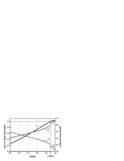
Figure 2: The ratio of the optimal Fisher information (solid line) and the optimal time allocation as a function of the fidelity $F$. The measurement time is divided into three periods: coincidence $t_{1}$ (plus signs), anti-coincidence $t_{2}$ (circles), and total flux $t_{3}$ (squares), which are normalized as $t_{1}+t_{2}+t_{3}=1$ in the plot.

The optimal asymptotic variance is $\frac{(2F+1)(2-2F)(\sqrt{2-2F}+\sqrt{1+2F})^{2}}{6\lambda t}$ when the threshold $F_{0}$ is less than the critical point $F_{1}$. This asymptotic variance is much better than that obtained by the modified visibility method. The ratio of the optimal asymptotic variance is given by

$$\frac{(\sqrt{2-2F}+\sqrt{1+2F})^{2}}{6}<1.$$ (93)

In the following, we give the optimal test of level $\alpha$ in the hypothesis testing (6). Assume that the threshold $F_{0}$ is less than the critical point $F_{1}$. In this case, we can apply testing of the hypothesis (36). First, we measure the count on the coincidence vectors for a period of $t_{1}=\frac{t\sqrt{2-2F_{0}}}{\sqrt{2F_{0}+1}+\sqrt{2-2F_{0}}}$, to obtain the total count $n_{1}$. Then, we measure the count on the anti-coincidence vectors for a period of $t_{2}=\frac{t\sqrt{2F_{0}+1}}{\sqrt{2F_{0}+1}+\sqrt{2-2F_{0}}}$ to obtain the total count $n_{2}$. Note that the optimal time allocation depends on the threshold of our hypothesis. Finally, we apply the UMP test of $\alpha$ of the hypothesis:

$$\begin{array}[]{ccc}H_{0}:p\geq\frac{\sqrt{2-2F_{0}}}{\sqrt{2-2F_{0}}+\sqrt{1+2F_{0}}}&\hbox{ versus }&H_{1}:p<\frac{\sqrt{2-2F_{0}}}{\sqrt{2-2F_{0}}+\sqrt{1+2F_{0}}}\end{array}$$

with the binomial distribution family $P_{p}^{n_{1}+n_{2}}$ to the data $n_{1}$. In this case, the likelihood ratio test with the risk probability $\alpha$ is almost equal to the test with the rejection region: $\{(n_{1},n_{2})|\frac{n_{2}}{n_{2}+n_{1}}\leq\frac{\sqrt{2-2F_{0}}}{\sqrt{2F_{0}+1}+\sqrt{2-2F_{0}}}+\frac{\Phi^{-1}(\alpha)}{\sqrt{2F_{0}+1}+\sqrt{2-2F_{0}}}\sqrt{\frac{\sqrt{2-2F_{0}}\sqrt{2F_{0}+1}}{n_{1}+n_{2}}}\}$ concerning the null hypothesis $H_{0}:F\leq F_{0}$. The p-value of this kind of tests is $\Phi(\frac{n_{2}\sqrt{2F_{0}+1}-n_{1}\sqrt{2-2F_{0}}}{\sqrt{(n_{1}+n_{2})\sqrt{2F_{0}+1}\sqrt{2-2F_{0}}}})$.

We can apply a similar testing for $F_{0}>F_{1}$. It is sufficient to replace the time allocation to $t_{1}=0$ $t_{2}=\frac{t\sqrt{6}}{\sqrt{6}+\sqrt{2(1-F_{0})}}$, $t_{3}=\frac{t\sqrt{2(1-F_{0})}}{\sqrt{6}+\sqrt{2(1-F_{0})}}$. In this case, the likelihood ratio test with the risk probability $\alpha$ is almost equal to the test with the rejection region: $\{(n_{2},n_{3})|\frac{n_{2}}{n_{2}+n_{3}}\leq\frac{\sqrt{1-F_{0}}}{\sqrt{3}+\sqrt{1-F_{0}}}+\frac{\Phi^{-1}(\alpha)}{\sqrt{3}+\sqrt{1-F_{0}}}\sqrt{\frac{\sqrt{1-F_{0}}\sqrt{3}}{n_{2}+n_{3}}}\}$ concerning the null hypothesis $H_{0}:F\leq F_{0}$. The p-value of this kind of tests is $\Phi(\frac{n_{2}\sqrt{3}-n_{3}\sqrt{1-F_{0}}}{\sqrt{(n_{2}+n_{3})\sqrt{1-F_{0}}\sqrt{3}}})$.

Next, we consider the case where the dark count parameter $\delta$ is known but is not negligible, the Fisher information matrix is given by

$$\left(\begin{array}[]{cc}\lambda(\frac{2\lambda t_{1}}{3(\lambda(2F+1)+6\delta)}+\frac{2\lambda t_{2}}{3(\lambda(2-2F)+6\delta)})&\frac{\lambda(2F+1)}{3(\lambda(2F+1)+6\delta)}t_{1}-\frac{\lambda(2-2F)}{3(\lambda(2-2F)+6\delta)}t_{2}\\ \frac{\lambda(2F+1)}{3(\lambda(2F+1)+6\delta)}t_{1}-\frac{\lambda(2-2F)}{3(\lambda(2-2F)+6\delta)}t_{2}&\frac{2F+1}{\lambda(2F+1)+6\delta}\frac{2F+1}{6}t_{1}+\frac{2-2F}{\lambda(2-2F)+6\delta}\frac{2-2F}{6}t_{2}+\frac{1}{\lambda}t_{3}\end{array}\right).$$ (96)

Hence, from (65), the inverse of the minimum variance is equal to

$$f(t_{1},t_{2},t_{3})$$

$$:= \lambda(\frac{2\lambda t_{1}}{3(\lambda(2F+1)+6\delta)}+\frac{2\lambda t_{2}}{3(\lambda(2-2F)+6\delta)}$$

$$-\frac{(\frac{\lambda(2F+1)}{3(\lambda(2F+1)+6\delta)}t_{1}-\frac{\lambda(2-2F)}{3(\lambda(2-2F)+6\delta)}t_{2})^{2}}{\frac{\lambda(2F+1)}{\lambda(2F+1)+6\delta}\frac{2F+1}{6}t_{1}+\frac{\lambda(2-2F)}{\lambda(2-2F)+6\delta}\frac{2-2F}{6}t_{2}+t_{3}}).$$

Then, we apply Lemmas 1 and 2 in Appendix A to $\frac{f(t_{1},t_{2},t_{3})}{\lambda}$ with $a=\frac{2\lambda}{3(\lambda(2F+1)+6\delta)}$, $b=\frac{2\lambda}{3(\lambda(2-2F)+6\delta)}$, $c=\frac{\lambda(2F+1)}{\lambda(2F+1)+6\delta}\frac{2F+1}{6}$, $d=\frac{\lambda(2-2F)}{\lambda(2-2F)+6\delta}\frac{2-2F}{6}$, and obtain the optimized value:

(i) coincidence and total flux

$$\max_{t_{1}+t_{3}=t}f(t_{1},0,t_{3}) =\frac{4\lambda t}{((2F+1)+\sqrt{\frac{6(\lambda(2F+1)+6\delta)}{\lambda}})^{2}}$$ (98)

(ii) anti-coincidence and total flux

$$\max_{t_{2}+t_{3}=t}f(0,t_{2},t_{3}) =\frac{4\lambda t}{((2-2F)+\sqrt{\frac{6(\lambda(2-2F)+6\delta)}{\lambda}})^{2}}$$ (99)

and

(iii) coincidence and anti-coincidence

$$\max_{t_{1}+t_{2}=t}f(t_{1},t_{2},0)= \lambda t\left(\frac{\frac{\lambda(2F+1)}{3\sqrt{(\lambda(2F+1)+6\delta)(\lambda(2-2F)+6\delta)}}+\frac{\lambda(2-2F)}{3\sqrt{(\lambda(2F+1)+6\delta)(\lambda(2-2F)+6\delta)}}}{(2F+1)\sqrt{\frac{\lambda}{6(\lambda(2F+1)+6\delta)}}+(2-2F)\sqrt{\frac{\lambda}{6(\lambda(2-2F)+6\delta)}}}\right)^{2}$$

$$= \frac{2\lambda^{2}t}{3(\lambda(2F+1)+6\delta)(\lambda(2-2F)+6\delta)}\left(\frac{3}{\frac{2F+1}{\sqrt{\lambda(2F+1)+6\delta}}+\frac{2-2F}{\sqrt{\lambda(2-2F)+6\delta}}}\right)^{2}$$

$$= \frac{6\lambda^{2}t}{\left((2F+1)\sqrt{\lambda(2-2F)+6\delta}+(2-2F)\sqrt{\lambda(2F+1)+6\delta}\right)^{2}}.$$ (101)

The ratio of (98) to (101) is

$$\frac{3\lambda\left((2F+1)+\sqrt{\frac{6(\lambda(2F+1)+6\delta)}{\lambda}}\right)^{2}}{2\left((2F+1)\sqrt{\lambda(2-2F)+6\delta}+(2-2F)\sqrt{\lambda(2F+1)+6\delta}\right)^{2}}$$

$$= \frac{3}{2}\left(\frac{(2F+1)\sqrt{\lambda}+\sqrt{6(\lambda(2F+1)+6\delta)}}{(2F+1)\sqrt{\lambda(2-2F)+6\delta}+(2-2F)\sqrt{\lambda(2F+1)+6\delta}}\right)^{2}>1,$$ (102)

where the final inequality is derived in Appendix B. Therefore, the measurement using the coincidence and the anti-coincidence provides better test than that using the coincidence and the total flux, as in the case of $\delta=0$.

Define $\delta_{1}$ and the critical point $F_{\delta^{\prime}}$ for the normalized dark count $\delta^{\prime}=6\delta/\lambda<\delta_{1}$ as

$$\sqrt{\delta_{1}+3}-\sqrt{\delta_{1}} =\sqrt{3/2}$$

$$\sqrt{1+2F_{\delta^{\prime}}+{\delta^{\prime}}}-\sqrt{2-2F_{\delta^{\prime}}+{\delta^{\prime}}} =\sqrt{3/2}.$$

The parameter $\delta_{1}$ is calculated to be $0.375$. As shown in Appendix C, the measurement using the coincidence and the anti-coincidence provides better test than that using the anti-coincidence and the total flux, if the fidelity is smaller than the critical point $F_{\delta^{\prime}}$:

$$\max_{t_{1}+t_{2}+t_{3}=t}f(t_{1},t_{2},t_{3})$$

$$= \left\{\begin{array}[]{ll}\frac{4\lambda^{2}t}{((2-2F)\sqrt{\lambda}+\sqrt{6(\lambda(2-2F)+6\delta)})^{2}}&\hbox{ if }F>F_{\delta^{\prime}}\\ \frac{6\lambda^{2}t}{\left((2F+1)\sqrt{\lambda(2-2F)+6\delta}+(2-2F)\sqrt{\lambda(2F+1)+6\delta}\right)^{2}}&\hbox{ otherwise}.\end{array}\right.$$ (105)

The optimal time allocation is given by $t_{1}=0$, $t_{2}=\frac{t\sqrt{6(\lambda(2-2F)+6\delta)}}{\sqrt{6(\lambda(2-2F)+6\delta)}+(2-2F)\sqrt{\lambda}}$, and $t_{3}=\frac{t(2-2F)\sqrt{\lambda}}{\sqrt{6(\lambda(2-2F)+6\delta)}+(2-2F)\sqrt{\lambda}}$ for $F>F_{\delta^{\prime}}$, and $t_{1}=\frac{t(2-2F)\sqrt{\lambda(2F+1)+6\delta}}{(2-2F)\sqrt{\lambda(2F+1)+6\delta}+(2F+1)\sqrt{\lambda(2-2F)+6\delta}}$, $t_{2}=\frac{t(2F+1)\sqrt{\lambda(2-2F)+6\delta}}{(2-2F)\sqrt{\lambda(2F+1)+6\delta}+(2F+1)\sqrt{\lambda(2-2F)+6\delta}}$, $t_{3}=0$ for $F\leq F_{\delta^{\prime}}$. The critical point $F_{\delta^{\prime}}$ for optimal time allocation increases with the normalized dark count as illustrated in Fig. 3.

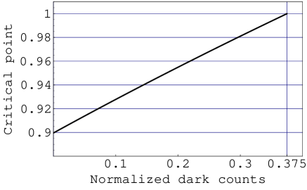
Figure 3: The critical point $F_{\delta^{\prime}}$ for optimal time allocation as a function of normalized dark counts $\delta^{\prime}$.

VIII Design II ($\lambda$: known, One Stage)

In this section, we consider the case where $\lambda$ is known. Then, the Fisher information is

$$\lambda(\frac{2\lambda t_{1}}{3(\lambda(2F+1)+6\delta)}+\frac{2\lambda t_{2}}{3(\lambda(2-2F)+6\delta)}).$$ (106)

The maximum value is calculated as

$$\max_{t_{1}+t_{2}+t_{3}=t}(\ref{2-24-1})=\left\{\begin{array}[]{ll}\frac{2\lambda^{2}t}{3(\lambda(2F+1)+6\delta)}&\hbox{ if }F<\frac{1}{4}\\ \frac{2\lambda^{2}t}{3(\lambda(2-2F)+6\delta)}&\hbox{ if }F\geq\frac{1}{4}.\end{array}\right.$$ (109)

The above optimization shows that when $F\geq\frac{1}{4}$, the count on anti-coincidence $(t_{1}=0;t_{2}=t;t_{3}=0)$ is better than the count on coincidence $(t_{1}=t;t_{2}=0;t_{3}=0)$. In fact, Barbieri et al.BMNMDM03 measured the sum of the counts on the anti-coincidence vectors $|HV\rangle,|VH\rangle,|DX\rangle,|XD\rangle,|RR\rangle,|LL\rangle$ to realize the entanglement witness in their experiment. In this case, the variance is $\frac{3(\lambda(2-2F)+6\delta)}{2\lambda^{2}t}$. When we observe the sum of counts on anti-coincidence $n_{2}$, the estimated value of $F$ is given by $1+3(\delta-\frac{n_{2}}{\lambda t})$, which is the solution of $(\lambda\frac{2-2F}{6}+\delta)t=n_{2}$. The likelihood ratio test with the risk probability $\alpha$ can be approximated by the test with the rejection region: $\{n_{2}|n_{2}\leq(\frac{\lambda(1-F_{0})}{3}+\delta)t+\Phi^{-1}(\alpha)\sqrt{(\frac{\lambda(1-F_{0})}{3}+\delta)t}\}$ concerning the null hypothesis $H_{0}:F\leq F_{0}$, which is also the UMP test. The p-value of likelihood ratio tests is $\Phi(\frac{n_{2}-(\frac{\lambda(1-F_{0})}{3}+\delta)t}{\sqrt{(\frac{\lambda(1-F_{0})}{3}+\delta)t}})$.

When $F<\frac{1}{4}$, the optimal time allocation is $t_{1}=t$, $t_{2}=t_{3}=0$. The fidelity is estimated by $\frac{3n_{2}}{\lambda t}-\frac{1}{2}$. Its variance is $\frac{3(\lambda(2F+1)+6\delta)}{2\lambda^{2}t}$. The likelihood ratio test with the risk probability $\alpha$ of the Poisson distribution is almost equal to the test with the rejection region: $\{n_{1}|n_{1}\geq(\lambda\frac{1+2F_{0}}{6}+\delta)t+\Phi^{-1}(1-\alpha)\sqrt{(\lambda\frac{1+2F_{0}}{6}+\delta)t}\}$ concerning the null hypothesis $H_{0}:F\leq F_{0}$, which is also the UMP test. The p-value of likelihood ratio tests is $\Phi(\frac{-n_{1}+(\lambda\frac{1+2F_{0}}{6}+\delta)t}{\sqrt{(\lambda\frac{1+2F_{0}}{6}+\delta)t}})$.

IX Comparison of the asymptotic variances

We compare the asymptotic variances of the following designs for time allocation, when the dark count $\delta$ parameter is zero.

(i)

Modified visibility: The asymptotic variance is $\frac{(2F+1)(2-2F)}{\lambda t}$.

(iia)

Design I ($\lambda$ unknown). optimal time allocation between the counts on anti-coincidence and coincidence: The asymptotic variance is $\frac{(2F+1)(2-2F)(\sqrt{2F+1}+\sqrt{2-2F})^{2}}{6\lambda t}$.

(iib)

Design I ($\lambda$ unknown), optimal time allocation between the counts on anti-coincidence and the total flux: The asymptotic variance is $\frac{(2-2F)(\sqrt{6}+\sqrt{2-2F})^{2}}{4\lambda t}$.

(iiia)

Design II ($\lambda$ known), estimation from the count on anti-coincidence: The asymptotic variance is $\frac{3(2-2F)}{2\lambda t}$.

(iiib)

Design II ($\lambda$ known), estimation from the count on coincidence: The asymptotic variance is $\frac{3(2F+1)}{2\lambda t}$.

Fig. 4 shows the comparison, where the asymptotic variances in (iia)-(iiib) are normalized by the one in (i). The anti-coincidence measurement provides the best estimation for high ($F>0.25$) fidelity. When $\lambda$ is unknown, the measurement with the counts on anti-coincidence and the coincidence is better than that with the counts anti-coincidence and the total flux for $F<0.899519$. For higher fidelity, the counts on anti-coincidence and total flux turns to be better, but the difference is small.

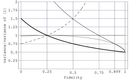
Figure 4: Comparison of the designs for time allocation. The asymptotic variances normalized by the value of modified visibility method are shown as a function of fidelity, where dots: (iia), solid: (iib), thick: (iiia), and dash: (iiib).

X Design III ($\lambda$: known, Two Stage)

X.1 Optimal Allocation

The comparison in the previous section shows that the measurement on the anti-coincidence vectors yields a better variance than the measurement on the coincidence vectors, when the fidelity is greater than $1/4$ and the parameters $\lambda$ and $\delta$ are known. We will explore further improvement in the measurement on the anti-coincidence vectors. In the previous sections, we allocate an equal time to the measurement on each of the anti-coincidence vectors. Here we minimize the variance by optimizing the time allocation $t_{HV}$, $t_{VH}$, $t_{DX}$, $t_{XD}$, $t_{RR}$, and $t_{LL}$ between the anti-coincidence vectors $B=\{|HV\rangle$, $|VH\rangle$, $|DX\rangle$, $|XD\rangle$, $|RR\rangle$, and $|LL\rangle\}$, under the restriction of the total measurement time: $\sum_{(x,y)\in B}t_{x,y}=t$. The number of the counts $n_{xy}$ obeys Poisson distribution Poi($(\lambda\mu_{xy}+\delta)t_{xy}$) with unknown parameter $\mu_{xy}$. Then, the Fisher information matrix is the diagonal matrix with the diagonal elements $\{\frac{\lambda^{2}t_{x,y}}{\lambda\mu_{x,y}+\delta}\}_{(x,y)\in B}$ Since we are interested in the parameter $1-F=\frac{1}{2}(\sum_{(x,y)\in B}\mu_{x,y})$, the variance is given by

$$\frac{1}{4}\Bigl{(}\sum_{(x,y)\in B}\frac{\lambda\mu_{x,y}+\delta}{\lambda^{2}t_{x,y}}\Bigr{)},$$ (110)

as mentioned in section V.1. Under the restriction of the total measurement time, the minimum value of (110) is

$$\frac{(\sum_{(x,y)\in B}\sqrt{\lambda\mu_{x,y}+\delta})^{2}}{4\lambda^{2}t},$$ (111)

which is attained by the optimal time allocation

$$t_{xy}=\frac{(\lambda\sqrt{\mu_{xy}}+\delta)t}{\sum_{(x^{\prime},y^{\prime})\in B}\sqrt{\lambda\mu_{x^{\prime},y^{\prime}}+\delta}},$$ (112)

which is called Neyman allocation and is used in sampling designCochran . The variance with the equal allocation is

$$\frac{3(\lambda(2-2F)+6\delta)}{2\lambda^{2}t}=\frac{3(\lambda(\sum_{(x,y)\in B}\mu_{x,y})+6\delta)}{2\lambda^{2}t}.$$ (113)

The inequality (111) $\leq$ (113) can be derived from Schwartz’s inequality of the vectors $(1,\ldots,1)$ and $(\sqrt{\lambda\mu_{HV}+\delta},\ldots,\sqrt{\lambda\mu_{LL}+\delta})$. The equality holds if and only if $\mu_{HV}=\mu_{VH}=\mu_{DX}=\mu_{XD}=\mu_{RR}=\mu_{LL}$. Therefore, the Neyman allocation has an advantage over the equal allocation, when there is a bias in the parameters $\mu_{HV},\mu_{VH},\mu_{DX},\mu_{XD},\mu_{RR},\mu_{LL}$. In other words, the Neyman allocation is effective when the expectation values of the counts on some vectors are larger than those on other vectors.

X.2 Two-stage Method

The optimal time allocation derived above is not applicable in the experiment, because it depends on the unknown parameters $\mu_{HV},$ $\mu_{VH},$ $\mu_{DX},$ $\mu_{XD},$ $\mu_{RR},$ and $\mu_{LL}$. In order to resolve this problem, we introduce a two-stage method, where the total measurement time $t$ is divided into $t_{f}$ for the first stage and $t_{s}$ for the second stage under the condition of $t=t_{f}+t_{s}$. In the first stage, we measure the counts on each vectors for $t_{f}/6$ and estimate the expectation value for Neyman allocation on measurement time $t_{s}$. In the second stage, we measure the counts on a vector $|x_{A}y_{B}\rangle$ according to the estimated Neyman allocation. The two-stage method is formulated as follows.
(i) The measurement time for each vector in the first stage is given by $t_{f}/6$
(ii) In the second stage, we measure the counts on a vector $|x_{A}y_{B}\rangle$ with the measurement time $\tilde{t}_{xy}$ defined as

$$\tilde{t}_{xy}=\frac{m_{xy}}{\sum_{(x,y)\in B}\sqrt{m_{xy}}}(t-t_{f})$$

where $m_{xy}$ is the observed count in the first stage.
(iii) Define $\hat{\mu}_{xy}$ and $\hat{F}$ as

$$\hat{\mu}_{xy}=\frac{n_{xy}}{\lambda\tilde{t}_{xy}},\quad\hat{F}=1-\frac{1}{2}\sum_{(x,y)\in B}\hat{\mu}_{x,y},$$

where $n_{x,y}$ is the number of the counts on $|x_{A}y_{B}\rangle$ for $\tilde{t}_{xy}$. Then, we can estimate the fidelity by $\hat{F}$.
(iv) Finally, we apply the test $\phi_{\mathop{\rm mod}\nolimits,\alpha}$ given in Section IV.4 to the two hypotheses given as

$$H_{0}:\vec{w}\cdot\vec{\mu}\geq c_{0}\mbox{ versus }H_{1}:\vec{w}\cdot\vec{\mu}<c_{0},$$ (114)

where $w_{x,y}:=\frac{1}{2\lambda\tilde{t}_{x,y}}$ and $c_{0}:=1-F_{0}$.

XI Conclusion

We have formulated the hypothesis testing scheme to test the entanglement in the Poisson distribution framework. Our statistical method can handle the fluctuation in the experimental data more properly in a realistic setting. It has been shown that the optimal time allocation improves the test: the measurement time should be allocated preferably to the anti-coincidence vectors. This test is valid even if the dark count exists. This design is particularly useful for the experimental test, because the optimal time allocation depends only on the threshold of the test. We don’t need any further information of the probability distribution and the tested state. The test can be further improved by optimizing time allocation between the anti-coincidence vectors, when the error from the maximally entangled state is anisotropic. However, this time allocation requires the expectation values on the counts on coincidence, so that we need to apply the two stage method.

Appendix A Optimization of Fisher information

In this section, we maximize the quantities appearing in Fisher information.

Lemma 1

The equation

$$\max_{t_{1},t_{3}\geq 0,~{}ct_{1}+t_{3}=t}at_{2}-\frac{act_{1}^{2}}{ct_{1}+t_{3}}=\frac{at}{(\sqrt{c}+1)^{2}}$$ (115)

holds and the maximum value is attained when $t_{1}=\frac{t}{\sqrt{c}+1}$, $t_{3}=\frac{\sqrt{c}t}{\sqrt{c}+1}$.

Proof: Letting $x:=ct_{1}+t_{3}$, we have $t_{1}=\frac{x-t}{c-1}$. Then,

$$at_{1}-\frac{act_{1}^{2}}{ct_{1}+t_{3}}=\frac{a}{(c-1)^{2}}\left(-x-\frac{ct^{2}}{x}+(c+1)t\right).$$

Hence, the maximum is attained at $x=\sqrt{c}t$, i.e., $t_{1}=\frac{t}{\sqrt{c}+1}$ and $t_{3}=\frac{t\sqrt{c}}{\sqrt{c}+1}$. Thus,

$$\max_{t_{1},t_{3}\geq 0,~{}ct_{1}+t_{3}=t}at_{1}-\frac{act_{1}^{2}}{ct_{1}+t_{3}}$$

$$= \frac{a}{(c-1)^{2}}\left(-2\sqrt{c}t+(c+1)t\right)=\frac{at}{(\sqrt{c}+1)^{2}}.$$

 

Lemma 2

The equation

$$\max_{t_{1},t_{2}\geq 0,~{}t_{1}+t_{2}=t}at_{1}+bt_{2}-\frac{(\sqrt{ac}t_{1}-\sqrt{bc}t_{2})^{2}}{ct_{1}+dt_{2}}$$

$$= \frac{t(\sqrt{ad}+\sqrt{bc})^{2}}{(\sqrt{c}+\sqrt{d})^{2}}.$$ (116)

holds, and this maximum value is attained when $t_{1}=\frac{t\sqrt{d}}{\sqrt{c}+\sqrt{d}}$, $t_{2}=\frac{t\sqrt{c}}{\sqrt{c}+\sqrt{d}}$.

Proof: Letting $x:=ct_{1}+dt_{2}$, we have $t_{1}=\frac{dt-x}{d-c}$ and

$t_{2}=\frac{x-ct}{d-c}$. Then,

$$at_{1}+bt_{2}-\frac{(\sqrt{ac}t_{1}-\sqrt{bc}t_{2})^{2}}{ct_{1}+dt_{2}}$$

$$= \left(\frac{\sqrt{ad}+\sqrt{bc}}{d-c}\right)^{2}\left((c+d)t-x-\frac{cdt^{2}}{x}\right).$$

Hence, the maximum is attained at $x=\sqrt{cd}t$, i.e., $t_{1}=\frac{t\sqrt{d}}{\sqrt{c}+\sqrt{d}}$ and $t_{2}=\frac{t\sqrt{c}}{\sqrt{c}+\sqrt{d}}$. Thus,

$$\max_{t_{1},t_{2}\geq 0,~{}t_{1}+t_{2}=t}at_{1}+bt_{2}-\frac{(\sqrt{ac}t_{1}-\sqrt{bd}t_{2})^{2}}{ct_{1}+dt_{2}}$$

$$= \left(\frac{\sqrt{ad}+\sqrt{bc}}{d-c}\right)^{2}\left((c+d)t-2\sqrt{cd}t\right)=\frac{t(\sqrt{ad}+\sqrt{bc})^{2}}{(\sqrt{c}+\sqrt{d})^{2}}.$$

 

Further, three-parameter case can be maximized as follows.

Lemma 3

The maximum value

$$\max_{t_{1},t_{2},t_{3}\geq 0,~{}t_{1}+t_{2}+t_{3}=t}at_{1}+bt_{2}-\frac{(\sqrt{ac}t_{1}-\sqrt{bd}t_{2})^{2}}{ct_{1}+dt_{2}+t_{3}}$$

is equal to the maximum among three values $\displaystyle\max_{t_{1},t_{3}\geq 0,~{}ct_{1}+t_{3}=t}at_{2}-\frac{act_{1}^{2}}{ct_{1}+t_{3}}$, $\displaystyle\max_{t_{2},t_{3}\geq 0,~{}ct_{2}+t_{3}=t}at_{2}-\frac{bdt_{2}^{2}}{dt_{2}+t_{3}}$, $\displaystyle\max_{t_{1},t_{2}\geq 0,~{}t_{1}+t_{2}=t}at_{1}+bt_{2}-\frac{(\sqrt{ac}t_{1}-\sqrt{bd}t_{2})^{2}}{ct_{1}+dt_{2}}$.

Proof: Define two parameters $x:=ct_{1}+dt_{2}+t_{3}$ and $y:=\sqrt{cd}t_{1}-\sqrt{bd}t_{2}$. Then, the range of $x$ and $y$ forms a convex set. Since

$$t_{1} =\frac{\sqrt{bd}(x-t)+(d-1)y}{\sqrt{bd}(c-1)+\sqrt{ac}(d-1)},$$

$$t_{2} =\frac{\sqrt{ac}(x-t)-(c-1)y}{\sqrt{ac}(c-1)+\sqrt{bd}(d-1)}.$$

Hence,

$$at_{1}+bt_{2}-\frac{(\sqrt{ac}t_{1}-\sqrt{bd}t_{2})^{2}}{ct_{1}+dt_{2}+t_{3}}$$

$$= \biggl{(}\frac{a\sqrt{bd}}{\sqrt{bd}(c-1)+\sqrt{ac}(d-1)}$$

$$\quad+\frac{b\sqrt{ac}}{\sqrt{ac}(c-1)+\sqrt{bd}(d-1)}\biggr{)}(x-t)$$

$$+\biggl{(}\frac{a(d-1)}{\sqrt{bd}(c-1)+\sqrt{ac}(d-1)}$$

$$\quad-\frac{b(c-1)}{\sqrt{ac}(c-1)+\sqrt{bd}(d-1)}\biggr{)}y-\frac{y^{2}}{x}$$

$$= -\frac{1}{x}(y-\frac{1}{2}Bx)^{2}+(\frac{B^{2}}{4}+A)x-At,$$

where $A:=\frac{a\sqrt{bd}}{\sqrt{bd}(c-1)+\sqrt{ac}(d-1)}+\frac{b\sqrt{ac}}{\sqrt{ac}(c-1)+\sqrt{bd}(d-1)}$, $B:=\frac{a(d-1)}{\sqrt{bd}(c-1)+\sqrt{ac}(d-1)}-\frac{b(c-1)}{\sqrt{ac}(c-1)+\sqrt{bd}(d-1)}$. Applying Lemma 4, we obtain this lemma.   

Lemma 4

Define the function $f(x,y):=-\frac{1}{x}(y-\alpha x)^{2}+\beta x$ on a closed convex set $C$. The maximum value is realized at the boundary $bdC$.

Proof: The condition can be classified to two cases: i) $bdC\cap\{y=\alpha x\}=\emptyset$, ii) $bdC\cap\{y=\alpha x\}\neq\emptyset$. In the case i), when fix $x$ is fixed, $\max_{y:(x,y)\in C}f(x,y)=\max_{y:(x,y)\in bdC}f(x,y)$. Then, we obtain $\max_{(x,y)\in C}f(x,y)=\max_{(x,y)\in bdC}f(x,y)$. In the case ii), when $(x,\alpha x)\in C$, $\max_{y:(x,y)\in C}f(x,y)=f(x,\alpha x)=\beta x$. Hence, $\max_{x:(x,\alpha x)\in C}\max_{y:(x,y)\in C}f(x,y)=\max_{x:(x,\alpha x)\in C}\beta x$ This maximum is attained at $x=\max_{x}\{x|:(x,\alpha x)\in C\}$ or $x=\min_{x}\{x|:(x,\alpha x)\in C\}$. These point belongs to the boundary $bdC$. Further, $\max_{x:(x,\alpha x)\notin C}\max_{y:(x,y)\in C}f(x,y)=\max_{x:(x,\alpha x)\in C}\max_{y:(x,y)\in bdC}f(x,y)$. Thus, the proof is completed.   

Appendix B Proof of Inequalities (88) and (102)

It is sufficient to show

$$\sqrt{\frac{3}{2}}\left((2F+1)\sqrt{\lambda}+\sqrt{6(\lambda(2F+1)+6\delta)}\right)$$

$$-\Bigl{(}(2F+1)\sqrt{\lambda(2-2F)+6\delta}$$

$$\quad+(2-2F)\sqrt{\lambda(2F+1)+6\delta}\Bigr{)}>0.$$ (117)

By putting $\delta^{\prime}:=\frac{6\delta}{\lambda}$, the LHS is evaluated as

$$\frac{\hbox{\rm LHS of }(\ref{2-24-22})}{\sqrt{\lambda}}$$

$$= \sqrt{\frac{3}{2}}(2F+1)+3\sqrt{(2F+1)+\delta^{\prime})}$$

$$-(2F+1)\sqrt{(2-2F)+\delta^{\prime}}-(2-2F)\sqrt{(2F+1)+\delta^{\prime}}$$

$$= \sqrt{\frac{3}{2}}(2F+1)+(2F+1)\sqrt{(2F+1)+\delta^{\prime})}$$

$$-(2F+1)\sqrt{(2-2F)+\delta^{\prime}}$$

$$= (2F+1)\left(\sqrt{\frac{3}{2}}+\sqrt{(2F+1)+\delta^{\prime})}-\sqrt{(2-2F)+\delta^{\prime}}\right).$$

Since $0\leq F\leq 1$, we have

$$\sqrt{\frac{3}{2}}+\sqrt{(2F+1)+\delta^{\prime})}-\sqrt{(2-2F)+\delta^{\prime}}$$

$$\geq \sqrt{\frac{3}{2}}+\sqrt{1+\delta^{\prime}}-\sqrt{2+\delta^{\prime}}.$$

Further, the function $\delta^{\prime}\to\sqrt{1+\delta^{\prime}}-\sqrt{2+\delta^{\prime}}$ $(\delta^{\prime}\in[0,\infty])$ has the minimum $\sqrt{1}-\sqrt{2}>-1>-\sqrt{\frac{3}{2}}$ at $\delta^{\prime}=0$. Hence, $\frac{\hbox{\rm LHS of }(\ref{2-24-22})}{\sqrt{\lambda}}>0$.

Appendix C Proof of Equations (91) and (105)

It is sufficient to show that

$$\sqrt{\frac{3}{2}}\left((2-2F)\sqrt{\lambda}+\sqrt{6(\lambda(2-2F)+6\delta)}\right)$$

$$-\Bigl{(}(2F+1)\sqrt{\lambda(2-2F)+6\delta}$$

$$\quad+(2-2F)\sqrt{\lambda(2F+1)+6\delta}\Bigr{)}>0$$ (118)

if and only if $\frac{6\delta}{\lambda}<\delta_{1}$ and $F\geq F_{\frac{6\delta}{\lambda}}$. By putting $\delta^{\prime}:=\frac{6\delta}{\lambda}$, the LHS of (118) is evaluated as

$$\frac{\hbox{\rm LHS of }(\ref{2-24-4})}{\sqrt{\lambda}}$$

$$= \sqrt{\frac{3}{2}}(2-2F)+3\sqrt{(2-2F)+\delta^{\prime})}$$

$$-(2F+1)\sqrt{(2-2F)+\delta^{\prime}}-(2-2F)\sqrt{(2F+1)+\delta^{\prime}}$$

$$= \sqrt{\frac{3}{2}}(2-2F)+(2-2F)\sqrt{(2-2F)+\delta^{\prime}}$$

$$-(2-2F)\sqrt{(2F+1)+\delta^{\prime}}$$

$$= (2-2F)\left(\sqrt{\frac{3}{2}}+\sqrt{(2-2F)+\delta^{\prime}}-\sqrt{(2F+1)+\delta^{\prime}}\right).$$

Since $0\leq F\leq 1$ and $\delta\geq 0$,

$$\sqrt{\frac{3}{2}}+\sqrt{(2-2F)+\delta^{\prime}}-\sqrt{(2F+1)+\delta^{\prime}}>0$$

if and only if $\delta_{1}>\delta^{\prime}$ and $F>F_{\delta^{\prime}}$.

Appendix D Proof of (57)

Define $\tilde{\mu}_{i}$ by

$$\min_{\vec{w}\cdot\vec{\mu}^{\prime}=c_{0}}D({\rm Poi}(0,\ldots,0,\tilde{\mu}_{i},0,\ldots,0)\|{\rm Poi}(\vec{\mu}^{\prime}))=R.$$

In fact, when $w_{i}a<c_{0}$,

$$\min_{\mu_{i}^{\prime}\geq 0:~{}\vec{w}\cdot\vec{\mu}^{\prime}=c_{0}}D({\rm Poi}(0,\ldots,0,a,0,\ldots,0)\|{\rm Poi}(\vec{\mu}^{\prime}))$$

$$= \min_{\mu_{i}^{\prime}\geq 0:~{}\vec{w}\cdot\vec{\mu}^{\prime}=c_{0}}\sum_{j=1}^{m}\mu_{j}^{\prime}-a+a\log\frac{a}{\mu_{i}^{\prime}}$$

$$= \min_{\alpha\geq 0,\beta\geq 0:~{}\mu_{i}\alpha+\mu_{M}\beta=c_{0}}\alpha+\beta-a+a\log\frac{a}{\alpha}$$

$$= \left\{\begin{array}[]{ll}\frac{c_{0}}{w_{i}}-a+a\log\frac{aw_{i}}{c_{0}}&\hbox{ if }a\geq\frac{c_{0}(w_{M}-w_{i})}{w_{M}w_{i}}\\ \frac{c_{0}}{w_{M}}+a\log\frac{w_{M}-w_{i}}{w_{M}}&\hbox{ if }a<\frac{c_{0}(w_{M}-w_{i})}{w_{M}w_{i}}.\end{array}\right.$$

This value is monotone decreasing concerning $a$. When $a=\frac{c_{0}(w_{M}-w_{i})}{w_{M}w_{i}}$, this value is $\frac{c_{0}}{w_{M}}-\frac{c_{0}(w_{M}-w_{i})}{w_{i}w_{M}}\log\frac{w_{M}-w_{i}}{w_{M}}$. Hence, the value $\tilde{\mu}_{i}$ coincides with the the value $\tilde{\mu}_{i}$ defined by (55) and (56).

Thus, the relation (57) follows from the relation

$$\min_{\vec{w}\cdot\vec{\mu}^{\prime}=c_{0}}D({\rm Poi}(p_{1}a_{1},\ldots,p_{m}a_{m})\|{\rm Poi}(\vec{\mu}^{\prime}))$$

$$\leq \sum_{i=1}^{m}p_{i}\displaystyle\min_{\vec{w}\cdot\vec{\mu}^{\prime}=c_{0}}D({\rm Poi}(0,\ldots,0,a_{i},0,\ldots,0)\|{\rm Poi}(\vec{\mu}^{\prime})).$$

We choose $\vec{\mu}^{\prime}_{i}$ such that $\min_{\vec{w}\cdot\vec{\mu}^{\prime}=c_{0}}D({\rm Poi}(0,\ldots,0,a_{i},0,\ldots,0)\|{\rm Poi}(\vec{\mu}^{\prime}))=D({\rm Poi}(0,\ldots,0,a_{i},0,\ldots,0)\|{\rm Poi}(\vec{\mu}^{\prime}_{i}))$. Then, the above inequality follows from Lemma 5 in the following way:

$$\sum_{i=1}^{m}p_{i}\min_{\vec{w}\cdot\vec{\mu}^{\prime}=c_{0}}D({\rm Poi}(0,\ldots,0,a_{i},0,\ldots,0)\|{\rm Poi}(\vec{\mu}^{\prime}))$$

$$= \sum_{i=1}^{m}p_{i}D({\rm Poi}(0,\ldots,0,a_{i},0,\ldots,0)\|{\rm Poi}(\vec{\mu}^{\prime}_{i}))$$

$$\geq D({\rm Poi}(p_{1}a_{1},\ldots,p_{m}a_{m})\|{\rm Poi}(\sum_{i=1}^{m}p_{i}\vec{\mu}^{\prime}_{i}))$$

$$\geq \min_{\vec{w}\cdot\vec{\mu}^{\prime}=c_{0}}D({\rm Poi}(p_{1}a_{1},\ldots,p_{m}a_{m})\|{\rm Poi}(\vec{\mu}^{\prime})).$$

Lemma 5

Any real number $0\leq p\leq 1$ and any four sequence of positive numbers $(\mu_{i})$, $(\nu_{i})$, $(\mu_{i}^{\prime})$, and $(\nu_{i}^{\prime})$ satisfy

$$p(\sum_{i=1}^{m}(\mu_{i}-\nu_{i})+\sum_{i=1}^{m}\nu_{i}\log\frac{\nu_{i}}{\mu_{i}})$$

$$+(1-p)(\sum_{i=1}^{m}(\mu_{i}^{\prime}-\nu_{i}^{\prime})+\sum_{i=1}^{m}\nu_{i}^{\prime}\log\frac{\nu_{i}^{\prime}}{\mu_{i}^{\prime}})$$

$$\geq \sum_{i=1}^{m}((p\mu_{i}+(1-p)\mu_{i}^{\prime})-p\nu_{i}+(1-p)\nu_{i}^{\prime}))$$

$$+\sum_{i=1}^{m}(p\nu_{i}+(1-p)\nu_{i}^{\prime})\log\frac{(p\nu_{i}+(1-p)\nu_{i}^{\prime})}{(p\mu_{i}+(1-p)\mu_{i}^{\prime})}.$$

Proof: It is sufficient to show

$$p(\sum_{i=1}^{m}\nu_{i}\log\frac{\nu_{i}}{\mu_{i}})+(1-p)(\sum_{i=1}^{m}\nu_{i}^{\prime}\log\frac{\nu_{i}^{\prime}}{\mu_{i}^{\prime}})$$

$$\geq \sum_{i=1}^{m}(p\nu_{i}+(1-p)\nu_{i}^{\prime})\log\frac{(p\nu_{i}+(1-p)\nu_{i}^{\prime})}{(p\mu_{i}+(1-p)\mu_{i}^{\prime})}.$$

The convexity of $-\log$ implies that

$$-\log(\frac{(p\mu_{i}+(1-p)\mu_{i}^{\prime})}{(p\nu_{i}+(1-p)\nu_{i}^{\prime})})$$

$$= -\log(\frac{p\nu_{i}}{(p\nu_{i}+(1-p)\nu_{i}^{\prime})}\frac{\mu_{i}}{\nu_{i}}+\frac{(1-p)\nu_{i}^{\prime}}{(p\nu_{i}+(1-p)\nu_{i}^{\prime})}\frac{\mu_{i}^{\prime}}{\nu_{i}^{\prime}})$$

$$\leq \frac{p\nu_{i}}{(p\nu_{i}+(1-p)\nu_{i}^{\prime})}\cdot-\log(\frac{\mu_{i}}{\nu_{i}})$$

$$+\frac{(1-p)\nu_{i}^{\prime}}{(p\nu_{i}+(1-p)\nu_{i}^{\prime})}\cdot-\log(\frac{\mu_{i}^{\prime}}{\nu_{i}^{\prime}}).$$

Hence,

$$p(\sum_{i=1}^{m}\nu_{i}\log\frac{\nu_{i}}{\mu_{i}})+(1-p)(\sum_{i=1}^{m}\nu_{i}^{\prime}\log\frac{\nu_{i}^{\prime}}{\mu_{i}^{\prime}})$$

$$= \sum_{i=1}^{m}(p\nu_{i}+(1-p)\nu_{i}^{\prime})\Bigl{(}\frac{p\nu_{i}}{(p\nu_{i}+(1-p)\nu_{i}^{\prime})}\cdot-\log(\frac{\mu_{i}}{\nu_{i}})$$

$$+\frac{(1-p)\nu_{i}^{\prime}}{(p\nu_{i}+(1-p)\nu_{i}^{\prime})}\cdot-\log(\frac{\mu_{i}^{\prime}}{\nu_{i}^{\prime}})\Bigr{)}$$

$$\geq -\sum_{i=1}^{m}(p\nu_{i}+(1-p)\nu_{i}^{\prime})\log\frac{(p\nu_{i}+(1-p)\nu_{i}^{\prime})}{(p\mu_{i}+(1-p)\mu_{i}^{\prime})}.$$

 

Appendix E Proof of (67)

Considering the shape of the graph $\frac{x}{\sqrt{y}}=a$, we can show that the minimum value $\min_{(x,y)\in C}\frac{x}{\sqrt{y}}$ can be attained by the boundary of $C$. Hence the boundary of the convex set $Co(R)$ is included by the union $\cup_{i\neq j}l_{i,j}$ of the lines $l_{i,j}=\{(tx_{i}(R)+(1-t)x_{j}(R),ty_{i}(R)+(1-t)y_{j}(R))|0\leq t\leq 1\}$. Taking the derivative of $\frac{tx_{i}(R)+(1-t)x_{j}(R)}{\sqrt{ty_{i}(R)+(1-t)y_{j}(R)}}$ concerning $t$, we obtain

$$\min_{t\in[0,1]}\frac{tx_{i}(R)+(1-t)x_{j}(R)}{\sqrt{ty_{i}(R)+(1-t)y_{j}(R)}}=z_{i,j}(R).$$ (119)

Hence, we obtain (67).

References

- (1) C.H. Bennett, G. Brassard, C. Crépeau, R. Jozsa, A. Peres, and W. K. Wootters, Phys. Rev. Lett. 70, 1895 (1993).
- (2) H.-J. Briegel, W. Dur, J.I. Cirac, and P. Zoller, Phys. Rev. Lett., 81, 5932 (1998).
- (3) C. W. Helstrom, Quantum detection and estimation theory, Academic Press (1976).
- (4) A. S. Holevo, Probabilistic and statistical aspects of quantum theory, North-Holland Publishing (1982).
- (5) M. Hayashi, Asymptotic Theory of Quantum Statistical Inference: Selected Papers, World Scientific (2005).
- (6) A. G. White, D. F. V. James, P. H. Eberhard, and P. G. Kwiat, Phys. Rev. Lett., 83, 3103 (1999).
- (7) M. Barbieri, F. De Martini, G. Di Nepi, P. Mataloni, G. M. D’Ariano, and C. Macchiavello, Phys. Rev. Lett., 91, 227901 (2003).
- (8) Y. Tsuda, K. Matsumoto, and M. Hayashi. “Hypothesis testing for a maximally entangled state,” quant-ph/0504203.
- (9) E. L. Lehmann, Testing statistical hypotheses, Second edition. Wiley (1986).
- (10) P. G. Kwiat, E. Waks, A. G. White, I. Appelbaum, and P.H. Eberhard, Phys. Rev. A, 60, 773(R) (1999).
- (11) K. Usami, Y. Nambu, Y. Tsuda, K. Matsumoto, and K. Nakamura, “Accuracy of quantum-state estimation utilizing Akaike’s information criterion,” Phys. Rev. A, 68, 022314 (2003).
- (12) S. Amari and H. Nagaoka, Methods of Information Geometry, (AMS & Oxford University Press, 2000).
- (13) W. G. Cochran, Sampling Techniques, third edition, John Wiley, (1977).
- (14) M. Hayashi, B.-S. Shi, A. Tomita, K. Matsumoto, Y. Tsuda, and Y.-K. Jiang: “Hypothesis testing for an entangled state produced by spontaneous parametric down conversion,” quant-ph/0603254.