Reduced coherence in double-slit diffraction of neutrons

Abstract

In diffraction experiments with particle beams, several effects lead to a fringe visibility reduction of the interference pattern. We theoretically describe the intensity one can measure in a double-slit setup and compare the results with the experimental data obtained with cold neutrons. Our conclusion is that for cold neutrons the fringe visibility reduction is due not to decoherence, but to initial incoherence.

I Introduction

We provide a theoretical description of the intensity pattern in double-slit experiments with neutrons, with specific attention to the cold neutron diffraction ($\lambda\leavevmode\nobreak\ \approx\leavevmode\nobreak\ 20\,\mathrm{\AA}$) carried out by Zeilinger et al. in 1988 zeil . The result we obtain is shown in Fig. 1.

Usually, the main problem in the analysis of diffraction experiments is to establish exactly which causes bring about the reduced coherence experimentally inferred from the detected signal. This effect can be produced both by the initial preparation of the beam (namely, the non-dynamical incoherence) and by the interaction of its constituting particles with the environment (namely, the dynamical decoherence) pfau ; alten ; wise ; giulini ; alicki ; pascazio ; alcim ; horn ; angel ; horn2 .

We find that in the experiment of Ref. zeil decoherence does not play any role in the fringe visibility reduction, which indeed is entirely due to incoherence of the source. This conclusion is opposite to that of Ref. angel , where it is claimed that decoherence is essential for explaining the data from zeil .

We provide calculations and numerical simulations in support of an unexpected incoherence cause, which we propose plays a role in explaining the experimental data of Ref. zeil . This cause is that the width of the wave function impinging on the double-slit is comparable with the size of the double-slit setup (i.e., the distance between the two slits and the slit apertures). We argue that this feature of the incoming wave function leads to a slight difference in transverse momentum between the two wave packets emanating from the grating, such that the centers of the packets move apart. This momentum difference was already suggested in Ref. angel , but no physical explanation was given. It proves relevant for fitting the data of Ref. zeil . Even though it does not reduce the fringe visibility, it can significantly affect the shape of the interference pattern, changing the overlap of the two packets and so the position of secondary minima and maxima.

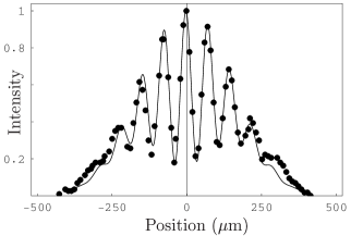
Figure 1: Comparison between theoretical prediction derived here (solid line) and experimental data taken from zeil (solid circles) for neutron double-slit diffraction.

II Visibility reduction in the intensity pattern

We now describe the various causes of reduced coherence which can occur within neutron interferometry. Let the $y$ direction be the direction of propagation of the beam. We assume that the grating is translation invariant in the $z$ direction, and that the motion in the $y$ direction is essentially classical, so that the problem reduces to one dimension, corresponding to the $x$ axis.

II.1 Initial incoherence

In the initial preparation of a beam, it is problematic to keep a perfect control on the monochromaticity and on the collimation of the beam.

Concerning the non-monochromaticity, every spectral component of the beam contributes incoherently to every other. In our case, assuming that the detection screen is parallel to the $x$ axis, the intensity observed on the screen at coordinate $x$ is

$$I(x)=\int\mathrm{d}\lambda\>f(\lambda)\>I_{\lambda}(x),$$ (1)

where $f(\lambda)\mathrm{d}\lambda$ is the wavelength distribution of the beam and $I_{\lambda}(x)$ the intensity corresponding to a single wavelength $\lambda$. Thus, one can continue the analysis with a single wavelength and postpone the integration (1) to the final step (see Sec. III).

Concerning the collimation of the beam, a relevant cause of incoherence is that the particle source emits random wave functions, whose randomness lies in the deviation of its direction of propagation from the $y$ direction, corresponding to imperfect collimation. This cause of incoherence will be taken into account in our model of the beam by means of a random wave vector $k$.

II.2 Decoherence

In the treatment of decoherence, we make explicit use of the fact that we are concerned with neutrons, in particular at the low energies of Ref. zeil . In this case, in fact, the only relevant decoherence channel—if any—consists in collisions with air molecules, so that the dynamics can be modelled within a Markovian description of the scattering event, in particular in the large scale approximation allowed by air molecules (see gallis ; giulini ; alcim ). The model obtained in this way allows an estimate of the neutron coherence time $\tau_{\rm coh}$ gallis ; alcim :

$$\tau_{\rm coh}=\frac{1}{P(\Theta_{\mathcal{E}})\,\sigma_{\rm tot}}\>\sqrt{\frac{8}{\pi\,k_{\scriptsize B}\,\Theta_{\mathcal{E}}\,m_{\rm air}}}\>,$$ (2)

where $P(\Theta_{\mathcal{E}})$ is the environmental pressure at the temperature $\Theta_{\mathcal{E}}$, $\sigma_{\rm tot}$ the total cross section of the scattering events, $k_{\scriptsize B}$ the Boltzmann constant and $\>m_{\rm air}\approx 4.8\cdot 10^{-26}\,\mathrm{Kg}$ the mean mass of air molecules. (Eq. (2) takes into account a correction by a factor $2\pi$, usually missing in the literature, that was theoretically predicted in sipe ; vacchini and experimentally checked in horn .)

The result is that $\tau_{\mathrm{coh}}$ is much greater than the time of flight, even in extreme experimental situations. In fact, even considering a surrounding pressure of $1\,\rm atm$ (though typically “the beam paths along the optical bench” are “evacuated in order to minimize absorption and scattering” zeil ) and room temperature, for an estimated total cross section of $10^{-27}\,\mathrm{m^{2}}$ we obtain that $\tau_{\rm coh}\approx 140\,\mathrm{s}$. This time—not much smaller than the neutron lifetime—shows that the coherence is fully kept for the duration of most experiments. For instance, in zeil the mean time of flight is $T\approx 0.023\,\mathrm{s}$, several orders of magnitude smaller than $\tau_{\mathrm{coh}}$.

For this reason, in the following we shall regard the neutron beam as uncoupled from its environment and shall describe the dynamics through the usual unitary Schrödinger evolution.

This conclusion contradicts that of Sanz et al. in Ref. angel , who claim that “decoherence is likely to exist in Zeilinger et al.’s experiment.” Indeed, their own calculations do not support their conclusion. The basis of their claim is that the damping term $\Lambda_{t}$ in their expression for the observed intensity pattern [see their Eq. (27)] turns out, when fitted to the data, to be nonzero. However, this term could just as well represent incoherence instead of decoherence (as does for example the similar quantity $\mathcal{A}$ in their Eq. (16), or the coherence length in Eq. (47) of Ref. alcim ) . Indeed, our estimate of the coherence time shows that the damping $\Lambda_{t}$ cannot be attributed to decoherence.

III Model for the intensity pattern

In order to obtain a theoretical description of the intensity pattern measured in the experiment, we precisely describe the whole evolution of the neutron beam, from its production to the arrival on the detection screen.

We set up a concrete model for what the wave functions of the neutrons in the beam look like, and thus obtain the density matrix and the intensity pattern. (Another approach englert is to guess the density matrix from information theoretic principles, but we prefer to avoid the invocation of such principles.)

The width $A$ of the entrance slit fixes the spatial extension of the (random) wave packets. The wave packets $\psi_{0}$ produced by the source are modeled, when passing the entrance slit, as Gaussian wave packets with mean $0$ and standard deviation $s_{0}=A/\sqrt{12}$, i.e., the standard deviation of the uniform probability distribution over the interval of length $A$. Thus,

$$\psi_{0}(x)\sim\exp\Bigl{(}-\frac{x^{2}}{2s_{0}^{2}}+ikx\Bigr{)},$$

where we take the random wave number $k$ to have a Gaussian distribution with mean 0 and standard deviation $\sigma_{k}$. As established in Sec. II.2, away from the grating, the neutrons follow the free Schrödinger evolution, so that—after the flight over the distance $L_{0}$—the packet just before the grating (the incoming wave function) has the Gaussian form

$$\psi_{\rm in}(x)\sim\exp\bigg{\{}-(1-i\gamma)\frac{\big{[}x-\delta(k)\big{]}^{2}}{2s^{2}}+ikx\bigg{\}},$$

with $\gamma=\lambda L_{0}/(4\pi s_{0}^{2})$, $s=s_{0}\sqrt{1+\gamma^{2}}$ and $\delta(k)=L_{0}\lambda k/(2\pi)$. In Sec. IV we shall present two different models for the wave function immediately after the grating (the outgoing wave function $\psi_{\rm out}$) as a function of the incoming wave function $\psi_{\rm in}$.

We now consider the free propagation of the outgoing state $\psi_{\rm out}$ toward the screen. We obtain the density matrix $\rho_{\mathrm{out}}$ by averaging $|\psi_{\mathrm{out}}\rangle\langle\psi_{\mathrm{out}}|$ with respect to the probability distribution of the wave number $k$. The intensity measured on the distant screen is proportional to the diagonal elements of the density matrix $\rho_{T}$ at the time of arrival $T=mL\lambda/(2\pi\hbar)$ (with $m$ the mass of the neutron)—as already stated and well motivated in the literature flux ; alcim : $I_{\lambda}(x)\sim\rho_{T}(x,x)$. Before identifying it with the measured intensity, we have also to consider the integration (1) over the wavelength and the finite spatial resolution $x_{0}$ of the detector. For the latter, we shall consider flat response on the interval $[x\!-\!x_{0}/2\,,\,x\!+\!x_{0}/2]$ around each position $x$, so that the intensity is finally given by

$$I(x)=\frac{1}{x_{0}}\int\!\mathrm{d}\lambda\>f(\lambda)\!\int_{x-x_{0}/2}^{x+x_{0}/2}\!\!\!\!\!\!\!\!\!\!\!\mathrm{d}y\>\>I_{\lambda}(y),$$

where $x_{0}$ and $f(\lambda)$ are directly adoptable from Ref. zeil .

IV Passage through the grating

We describe two models for the passage of the neutron through the grating. The first is a simplified model, which can be treated analytically and features the momentum difference between the two transmitted packets in the transverse $x$ direction. The second, on which Fig. 1 is based, is more flexible and achieves better agreement with experimental data.

IV.1 First model

The central assumption of this model is that the outgoing wave function is of the form

$$\psi_{\rm out}(x)=F(x)\psi_{\rm in}(x),$$

where $F$ is a complex function whose modulus is $\leq 1$ and signifies the degree of transmission, while the phase signifies the phase shift during the passage through the grating. The simplest model assumption would be to set $F(x)=1$ for $x\in[x_{1}-a_{1}/2,x_{1}+a_{1}/2]\cup[x_{2}-a_{2}/2,x_{2}+a_{2}/2]$ and $F(x)=0$ otherwise, where the two intervals represent the two slits, their apertures $a_{1}$, $a_{2}$ and distance $d$ are known zeil , and $x_{j}=(-1)^{j}(a_{j}+d)/2$ for $j=1,2$ is the center of the $j$-th slit. With this choice of $F$, the multiplication by $F$ is a projection operator. However, to enable analytical computations we find it more useful to set

$$F(x)\sim\frac{1}{\sigma_{1}}\exp\bigg{[}-\frac{(x-x_{1})^{2}}{2\sigma_{1}^{2}}\Big{]}+\frac{1}{\sigma_{2}}\exp\Big{[}-\frac{(x-x_{2})^{2}}{2\sigma_{2}^{2}}\bigg{]},$$

where $\sigma_{j}=a_{j}/\sqrt{12}$.

Now $I_{\lambda}(x)$ can be calculated exactly. In Fig. 2 the comparison between the theoretical intensity which follows from this model and the experimental data of Ref. zeil is shown. Apart from a constant background subtracted from experimental data, there is only one fit parameter $\sigma_{k}$, for which we have found $\sigma_{k}=10^{5}\,\mathrm{m/s}$. This value corresponds to a $x-$velocity with standard deviation equal to $0.006\,\mathrm{m/s}$, while the mean $y-$velocity distribution is $214\,\mathrm{m/s}$ zeil .

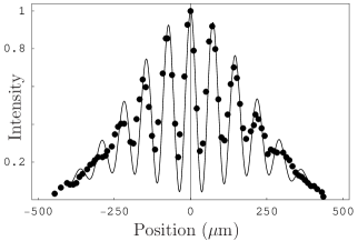
Figure 2: Comparison between the theoretical prediction derived with our first model for the passage through the grating (solid line) and experimental data taken from zeil (solid circles).

It is useful to look at the explicit formula for the outgoing wave function. For simplicity, set $k=0$. Then

$$\psi_{\rm out}(x)=\psi_{{\rm out},1}(x)+\psi_{{\rm out},2}(x),$$

where

$$\psi_{{\rm out},j}(x)\sim\exp\Big{[}-(x-\xi_{j})^{2}(\alpha_{j}-\frac{i\gamma}{2s^{2}})+\frac{ip_{j}x}{\hbar}\Big{]}$$

and where we have introduced the following quantities, for $j=1,2$: $\alpha_{j}=1/(2s^{2})+1/(2\sigma_{j}^{2})$, $\xi_{j}=x_{j}/(2\alpha_{j}\sigma_{j}^{2})$ and $p_{j}=\hbar\gamma x_{j}/(\sigma_{j}^{2}+s^{2})$. Therefore $\psi_{\rm out}$ is the sum of two Gaussian packets with momentum in the $x$ direction equal to $p_{1}$ and $p_{2}$. Moreover, since $x_{1}$ and $x_{2}$ have opposite signs, the same holds for $\xi_{1}$ and $\xi_{2}$ and, consequently, for $p_{1}$ and $p_{2}$. In other words, the packets produced by the grating have two opposite momenta in the transverse direction, as a consequence of the finite width of the neutron wave function compared to the scale fixed by the grating size. (Note that if $\psi_{\rm in}$ is very spread out, i.e., if $s$ is large, then $p_{j}\sim(\sigma_{j}^{2}+s^{2})^{-1}$ is small).

Also in the presence of a common drift expressed by $k$, the packets produced by the grating have wave number in the transverse direction equal to $k+p_{1}/\hbar$ and $k+p_{2}/\hbar$, with analytical expressions for the wave functions and $p_{j}$ more complicated than before.

Even though the agreement with experimental data is not completely satisfactory, this model illustrates the origin of the transverse momenta $p_{1}$ and $p_{2}$ that, as already noticed by Sanz et al. in Ref. angel , move outwards the $x-$position of secondary minima.

The values $p_{j}$ can also be predicted numerically by solving the Schrödinger equation for the passage of the neutron through the grating, treating the problem as two-dimensional with the double-slit modelled as an impenetrable potential barrier. Our numerical simulations were not accurate enough to yield realistic values, but did confirm that the $p_{j}$ are effectively nonzero, point in opposite directions (outwards), and have roughly equal modulus. Numerical simulations also suggest that the values of $p_{j}$ are substantially the same for all $\lambda$ within the range of wave lengths selected for the experiment.

IV.2 Second model

The second model allows to fit $p_{1}$ and $p_{2}$ to the data. It is based on the assumption that the outgoing wave function is of the form

$$\psi_{\mathrm{out}}(x)=c_{1}\,\varphi_{1}(x)+c_{2}\,\varphi_{2}(x)\,,$$

where $c_{j}\,\varphi_{j}$ is the wave packet emanating from the left ($j=1$) or right ($j=2$) slit, which we assume to be of Gaussian form:

$$\varphi_{j}(x)=\frac{1}{(2\pi\sigma_{j}^{2})^{1/4}}e^{-(x-x_{j})^{2}/4\sigma_{j}^{2}}\,e^{ik_{j}x}$$

allowing for the possibility that the drift $k_{j}$ and the weight $c_{j}$ are not equal for the two packets, where $\sigma_{j}$ and $x_{j}$ are the same quantities as introduced in Sec. IV.1.

We write the wave numbers $k_{j}$ as $k_{j}=k+p_{j}/\hbar$, i.e., the sum of the wave number $k$ of the incoming packet and the transverse momentum $p_{j}$ acquired during the passage through the grating, as previously highlighted.

We estimate the coefficients $c_{j}$ as

$$c_{j}=c_{j}(k)=\big{|}\psi_{\rm in}(x_{j})\big{|}\,.$$

Thus the wave packet emanating from slit 1 has greater weight $|c_{1}|^{2}$ if the incoming wave packet is closer to slit 1. (For further discussion see Ref. tesi .)

Fig. 1 shows the resulting prediction of this model. The following parameters were obtained by means of a fit procedure: the two velocities $p_{1}/m=-0.0034\,\mathrm{m/s}$ and $p_{2}/m=0.0029\,\mathrm{m/s}$ , and the angular divergence of the beam $\sigma_{k}=4976\,\mathrm{m}^{-1}$ (which corresponds to a $x-$velocity distribution with standard deviation equal to $0.0003\,\mathrm{m/s}$). Moreover, also in this case a constant background has been subtracted from experimental data. The $p_{j}$ have been assumed to be the same for all wave lenghts $\lambda$ selected for the experiment.

References

- (1) A. Zeilinger, R. Gähler, C. G. Shull, W. Treimer, and W. Mampe, Rev. Mod. Phys. 60, 1067 (1988).
- (2) E. Joos, H. D. Zeh, C. Kiefer, D. Giulini, J. Kupsch, and I.-O. Stamatescu, Decoherence and the Appearance of a Classical World in Quantum Theory, Second Edition, Springer, Berlin (2003).
- (3) T. Pfau, S. Spälter, Ch. Kurtsiefer, C. R. Ekstrom, and J. Mlynek, Phys. Rev. Lett. 73, 1223 (1994).
- (4) H. M. Wiseman, Phys. Rev. A 56, 2068 (1997).
- (5) T. P. Altenmüller, R. Müller, and A.Schenzle, Phys. Rev. A 56, 2959 (1997).
- (6) R. Alicki, Phys. Rev. A 65, 034104 (2002).
- (7) P. Facchi, A. Mariano, S. Pascazio, Recent Res. Dev. Phys. 3, 1 (2002); quant-ph/0105110.
- (8) A. Viale, M. Vicari, and N. Zanghì, Phys. Rev. A. 68, 063610 (2003).
- (9) K. Hornberger, J. E. Sipe, and M. Arndt, Phys. Rev. A 70, 053608 (2004).
- (10) K. Hornberger, L. Hackermüller, and M. Arndt, Phys. Rev. A 71, 023601 (2005); K. Hornberger, Phys. Rev. A 73, 052102 (2006).
- (11) A. S. Sanz, F. Borondo, and M. J. Bastiaans, Phys. Rev. A 71, 042103 (2005).
- (12) M. Daumer, D. Dürr, S. Goldstein, and N. Zanghì, J. Stat. Phys. 88, 967 (1997).
- (13) B. G. Englert, C. Miniatura, and J. Baudon, J. Phys. II France 4, 2043 (1994).
- (14) M. R. Gallis and G. N. Fleming, Phys. Rev. A 42, 38 (1990).
- (15) K. Hornberger and J. E. Sipe, Phys. Rev. A 68, 012105 (2003).
- (16) B. Vacchini, J. Mod. Opt. 51, 1025 (2004).
- (17) H. Palevsky and R. M. Eisberg, Phys. Rev. 98, 492 (1955); T. J. Krieger and M. S. Nelkin, Phys. Rev. 106, 290 (1957); J. A. Young and J. U. Koppel, Phys. Rev. 135, 603 (1964).
- (18) A. Viale, Loss of coherence in matter wave interferometry, Ph.D. dissertation, Department of Physics, University of Genoa, Italy (2006).