Unconditional security at a low cost

Abstract

By simulating four quantum key distribution (QKD) experiments and analyzing one decoy-state QKD experiment, we compare two data post-processing schemes based on security against individual attack by Lütkenhaus, and unconditional security analysis by Gottesman-Lo-Lütkenhaus-Preskill. Our results show that these two schemes yield close performances. Since the Holy Grail of QKD is its unconditional security, we conclude that one is better off considering unconditional security, rather than restricting to individual attacks.

I Introduction

Quantum key distribution (QKD) [1, 2] allows two parties, a transmitter Alice and a receiver Bob, to create a random secret key even when the channel is accessible to an eavesdropper, Eve. The security of QKD is built on the fundamental laws of physics in contrast to existing classical public key encryption schemes that are based on unproven computational assumptions. The unconditional security of the idealized QKD system has been proven in the past decade [3, 4, 5, 6].

In Shor-Preskill’s proof [5], two steps of data post-processing, error correction and privacy amplification, need to be performed in order to distill a secret key. Error correction ensures that Alice and Bob share an identical key, while privacy amplification removes Eve’s information about the final key. Alice and Bob can simply estimate the quantum bit error rate (QBER) by error testing and then perform error correction. Privacy amplification, on the other hand, requires the phase error rate which cannot be measured directly without a quantum computer. When an idealized QKD system is used, due to the symmetry of BB84, one can assume the phase error rate to be the same as the QBER [5]. However, any real QKD setup is not ideal but with imperfect sources, noisy channels and inefficient detectors, which will affect the security. To do security analysis, we should take these effects into consideration.

A few theoretical works have been done to deal with the imperfect devices, such as [7, 8, 9, 10, 11, 12, 13]. We will compare Lütkenhaus’ analysis [8] which deals with individual attacks and Gottesman-Lo-Lütkenhaus-Preskill (GLLP) [13] unconditional security proof. For convenience, we name the data post-procesing schemes, based on these two security analyses, after Lütkenhaus and GLLP.

Meanwhile, many QKD experiments [14, 15, 16, 17, 18] have been performed in the past decade. Experimentalists sometimes use the QBER as the only criterion for the security of QKD. However, after taking the imperfections into consideration, this kind of security analysis is incomplete. In fact, due to photon-number splitting (PNS) attacks [19, 9, 20], Eve can successfully break down the security even when the QBER is 0%.

Decoy states have been proposed as a useful method for substantially improving the performance of QKD with coherent sources [21]. The security proof of decoy-state QKD is given in Ref. [22]. Afterwards, some practical decoy-state protocols are proposed [23, 24, 25]. Recently, a few decoy-state QKD experiments have been performed [26, 27, 28, 29]. In this paper, we will consider both decoy-state and non-decoy-state cases.

The goal of this paper is to compare the two standard security proof results—Lütkenhaus and GLLP. We find that for realistic experimental parameters, with or without decoy states, the two security proof results give similar key generation rate and secure distance. Since unconditional security is the Holy Grail of QKD and GLLP (but not Lütkenhaus) gives unconditional security, our conclusion is that one should use GLLP as the standard criterion for security.

In Section II we review a widely used QKD model to real experiments. In Section III, we will compare two data post-processing schems, Lütkenhaus and GLLP for non-decoy and decoy-state QKD.

II Preliminaries

Here we use a QKD model following [8], see also [25]. We do not repeat the details of the model here. To reproduce the simulation results, one may need to refer to Section II of [25].

The procedure of a QKD experiment, using BB84 protocol with coherent state, is as follows:

1. In total, Alice sends Bob $N$ pulses for QKD, containing $N_{\mu}$ pulses for key transmission (signal states) and $N-N_{\mu}$ pulses for error testing or decoy states. In the $N_{\mu}$ signal pulses, Alice and Bob have $N_{\mu}^{s}$ pulses using same bases (after basis reconciliation).

2. Within the $N_{\mu}^{s}$ pulses, Bob gets a sifted key with a length of $K_{\mu}^{s}$, where they measure the same bases and Bob gets detections.

3. Alice and Bob choose a security analysis and perform a data post-processing scheme.

Here we assume Alice uses a weak coherent state for key transmission. Define the expected photon number (intensity) of the weak coherent state as $\mu$.

Define $q=N_{\mu}^{s}/N$. In BB84 scheme, $q=1/2$ when $N\rightarrow\infty$. Here subscript $\mu$ is the expected photon number of the coherent light used for key transmission as defined above.

Define the gain $Q_{\mu}=K_{\mu}^{s}/N_{\mu}^{s}$, the probability for Bob to get a detection in a pulse that Alice and Bob use the same basis.

Define the QBER $E_{\mu}=K_{\mu}^{err}/K_{\mu}^{s}$, the probability for Bob to get a wrong detection in a pulse that Alice and Bob use the same basis. Here $K_{\mu}^{err}$ is the number of erroneous bits in the sifted key.

Alice knows what $N$ and $\mu$ she uses for the key transmission. $N_{\mu}^{s}$ and $K_{\mu}^{s}$ can be directly counted from the data after the key transmission. Alice and Bob can estimate QBER from error testing, or they can count $K_{\mu}^{err}$ after error correction. In fact, even without knowing the real QBER, they can directly apply a error correction scheme (e.g., the Cascade scheme [30]). If the error correction is successful, then it automatically provides the QBER, otherwise they restart the QKD. Thus, in a real QKD system, Alice and Bob may skip the error testing part.

Assuming that the phase of each pulse is totally randomized, the photon number of each pulse follows a Poisson distribution with a parameter $\mu$ as its expected photon number. We remark that the phase randomization procedure is crucial for the security of QKD [31]. The density matrix of the state emitted by Alice is given by

$$\rho_{A}=\sum^{\infty}_{i=0}\frac{\mu^{i}}{i!}\,e^{-\mu}\,|i\rangle\langle i|,$$ (1)

where $|0\rangle\langle 0|$ is the vacuum state and $|i\rangle\langle i|$ is the $i$-photon state for $i=1,2\cdots$. The states with only one photon ($i=1$) are called single photon states. The states with more than one photon ($i\geq 2$) are called multi photon states.

Define $Y_{i}$ to be the yield of an $i$-photon state, i.e., the conditional probability of a detection event at Bob’s detector given that Alice sends out an $i$-photon state. Note that $Y_{0}$ is the background rate including detector dark counts and other background contributions such as the stray light in the fiber. Consequently, define the error rate of $i$-photon state to be $e_{i}$. The gain of $i$-photon states $Q_{i}$ is given by

$$Q_{i} =Y_{i}\frac{\mu^{i}}{i!}e^{-\mu}.$$ (2)

When $i=1$, $Q_{1}$ and $e_{1}$ are the gain and error rate of single photon states. Note that Eve has the ability to change $\{Y_{i}\}$ and $\{e_{i}\}$ as she wishes, but she cannot change $\mu$, which is set by Alice. Decoy states allow Alice and Bob to estimate channel transmittance and error rate accurately, which will restrict the Eve’s freedom to adjust $\{Y_{i}\}$ and $\{e_{i}\}$. This is the key reason why decoy states are useful for QKD [22].

III Data post-processing schemes

In this section, we will compare two data post-processing schemes, Lütkenhaus versus GLLP. During the comparison, we will apply two data post-processing schemes to both non-decoy and decoy state QKD.

III-A Lütkenhaus versus GLLP

Here we compare data post-processing schemes based on two security analyses, Lütkenhaus [8] and GLLP [13]. Lütkenhaus scheme focuses on security against individual attacks, while GLLP scheme proves unconditional security.

In the GLLP [13], there are so called tagged qubits in the discussion. The basis information of tagged qubits is somehow revealed to Eve. Thus tagged qubits are insecure for QKD. The idea is that Alice and Bob can (in principle) separate the qubits into two groups, tagged and untagged qubits, hence they only need to perform privacy amplification to the untagged qubits. The reason is as follows. The final key will be bitwise $XOR$ of keys that could be obtained from the tagged and untagged qubits. If the key from untagged qubits is private and random, then it doesn’t matter if Eve knows everything about tagged qubits — the sum is still private and random.

Based on the tagged qubit idea, the procedure of the data post-processing is as follows. First, Alice and Bob perform the error correction, and if it is successfully done, they share an identical key. And then they calculate how much privacy amplification they should do (according to certain security analysis, which we will discuss soon). Finally they use random hashing (or other privacy amplification procedure) to get a final secure key.

Due to PNS attack, we can regard qubits single photon states as untagged qubits and those from other (vacuum and multi photon) states as tagged qubits. Then we can compare the results of Lütkenhaus and GLLP schemes. We can rewrite the formula of the key generation rate by Lütkenhaus scheme

$$R\geq q\{-Q_{\mu}H_{2}(E_{\mu})+Q_{1}[1-\log_{2}(1+4e_{1}-4e_{1}^{2})]\}.$$ (3)

Similarly, as given in Eq. (11) in [22], we rewrite the key rate formula of GLLP

$$R\geq q\{-Q_{\mu}H_{2}(E_{\mu})+Q_{1}[1-H_{2}(e_{1})]\}$$ (4)

where $Q_{1}$ and $e_{1}$ are the gain and error rate of single photon states, and $H_{2}(x)=-x\log_{2}(x)-(1-x)\log_{2}(1-x)$ is the binary entropy function. Alice and Bob need to estimate $Q_{1}$ and $e_{1}$ given the data from QKD experiments.

In both Eqs. (3) and (4), the first term in the bracket is for error correction and the second one is for privacy amplification. The privacy amplification is only performed on the single photon part. In this manner, Lütkenhaus [8] has already applied the tagged qubits idea.

Here due to PNS attacks [19, 9, 20], both Lütkenhaus and GLLP assume that the single photon states are the only source of untagged qubits for BB84. This may not true for other protocols. For example, in SARG04 [32, 33], two-photon states can be used to extract secure keys.

Here is the key point of the whole paper. The difference between the Lütkenhaus and GLLP results appears in the privacy amplification part. We compare $H_{2}(e)$ with $\log_{2}(1+4e_{1}-4e_{1}^{2})$ in Fig. 1. We can see that the difference of two functions are quite small. For this reason, in fact, Lütkenhaus and GLLP give very similar result in the key generation rate and distance of secure QKD. In what follows, we will illustrate this crucial point with examples of experimental parameters from previous QKD experiments. Our conclusion holds with and without using decoy states.

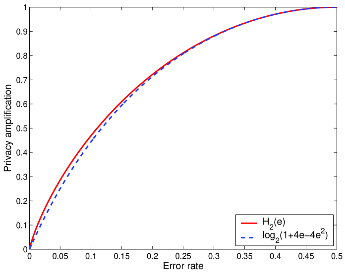
Figure 1: GLLP vs. Lütkenhaus. The maximal deviation of two curves is 15.36% when the error rate is 3.85%.

III-B Non-decoy-state QKD

Without decoy states, Alice and Bob have to pessimistically assume that all losses and errors come from single photon states. Thus

$$Q_{1} =Q_{\mu}-p_{M}$$ (5)

$$e_{1} =\frac{Q_{\mu}E_{\mu}}{Q_{1}}$$

where $p_{M}=1-(1+\mu)\exp(-\mu)$ is the probability that Alice sends out a multi photon state. We can recover Eq. (15) in [8] by substituting Eq. (5) into Eq. (3). Let $\Delta=p_{M}/Q_{\mu}$, we can recover Eq. (50) in [13] by substituting Eq. (5) into Eq. (4).

We compare the key generation rate of two data post-processing schemes based on Lütkenhaus and GLLP by simulating four experiment setups [15, 16, 17, 18]. The key parameters are listed in TABLE I.

	T8[15]	G13[16]	KTH[17]	GYS[18]
$\lambda$ [nm]	830	1300	1550	1550
$\alpha$ [dB/km]	2.5	0.32	0.2	0.21
$e_{d}$ [%]	1	0.14	1	3.3
$Y_{0}$ [/pulse]	$10^{-7}$	$1.64\times 10^{-4}$	$4\times 10^{-4}$	$1.7\times 10^{-6}$
$\eta_{Bob}$ [%]	7.92	8.14	14.30	4.5

TABLE I: Key parameters from four QKD experiment setups.

Fig. 2 shows the relationship between key generation rate and the transmission distance, comparing two data post-processing schemes, Lütkenhaus and GLLP. For both schemes, we consider non-decoy state QKD. From Fig. 2, we can see that the key generation rate of GLLP is only slightly lower than that of Lütkenhaus. Here we emphasize that GLLP deals with the general attack, while Lütkenhaus is restricted to individual attack.

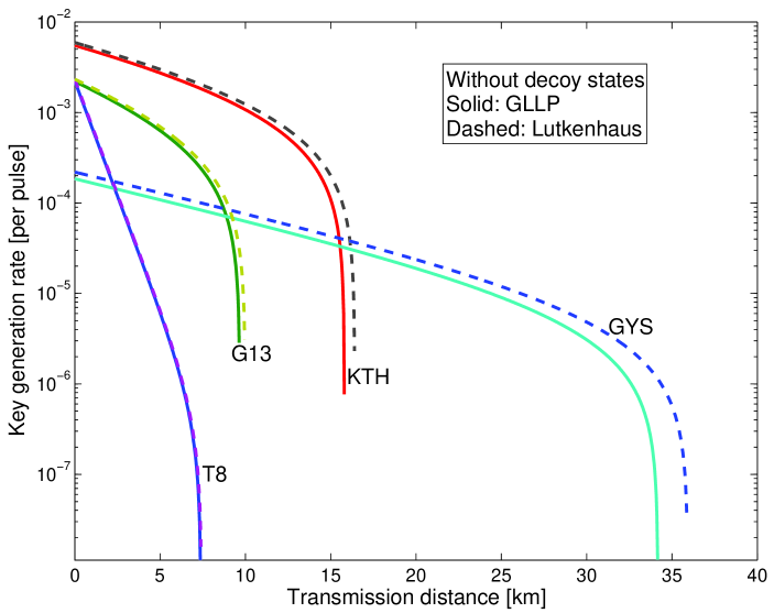
Figure 2: shows the relationship between key generation rate and the transmission distance, comparing two data post-processing schemes based on Lütkenhaus and GLLP security analyses. The key parameters are listed in TABLE I. Here we consider non-decoy case and use the optimal expected photon number $\mu=\eta$ [8]. Using Cascade protocol [30], the error correction efficiency is 1.16. Details of the QKD simulation model appear in [25].

We remark that the QBERs ($E_{\mu}$’s) of four GLLP curves at maximal distances in Fig. 2 are $4.57\%$, $4.80\%$, $4.80\%$ and $4.34\%$. Clearly it is far away from $11\%$, the tolerable QBER given in [5]. This is due to the fact that the QKD source is weak coherent state, while the security proof given in [5] is based on single photon source.

Many of QKD experiments used $\mu=0.1$ as for key transmission. If using $\mu=0.1$ for GYS [18] setup, we find that $Q_{\mu}<p_{M}$ for all transmission distances. That is, for BB84, Eve can successfully perform PNS attacks [19, 9, 20] and obtain all the information about the key even when the QBER is 0%!

III-C Decoy-state QKD

Here, we will give a data post-processing scheme following the security analysis of decoy state QKD [22].

In Eqs. (3) and (4), $q$ and $Q_{\mu}$ can be directly counted from Bob’s detection events. The QBER $E_{\mu}$ can be obtained from error testing or after error correction step. Alice and Bob can estimate $Q_{1}$ and $e_{1}$ with decoy states. Definitions of these variables are in Section II.

As for Vacuum+Weak decoy state scheme [25], besides $Q_{\mu}$ and $E_{\mu}$ discussed in Section II, Alice and Bob will use $Q_{vac}$ (from the vacuum decoy), $Q_{\nu}$ and $E_{\nu}$ (from the weak decoy). The definitions are similar as $Q_{\mu}$ and $E_{\mu}$ in Section II. The intensity of weak decoy state is $\nu$. Alice and Bob can publicly compare all weak decoy states to get $Q_{\nu}$ and $E_{\nu}$. They can estimate the background count rate by vacuum decoy states $Y_{0}=Q_{vac}$. Then, they apply the formulas, Eq. (35) and Eq. (37) in [25], for the estimations of $Q_{1}$ and $e_{1}$

$$Q_{1} \geq\frac{\mu^{2}e^{-\mu}}{\mu\nu-\nu^{2}}(Q_{\nu}e^{\nu}-Q_{\mu}e^{\mu}\frac{\nu^{2}}{\mu^{2}}-\frac{\mu^{2}-\nu^{2}}{\mu^{2}}Y_{0})$$ (6)

$$e_{1} \leq\frac{E_{\nu}Q_{\nu}e^{\nu}-e_{0}Y_{0}}{Q_{1}e^{\mu}\nu/\mu},$$

where $e_{0}=1/2$ is the error rate of vacuum decoy states.

In summary, the data post-processing for decoy state QKD is

1. Alice announces to Bob which pulses are used for decoy states. They publicly compare all values of decoy states, and then calculate $Q_{vac}$, $Q_{\nu}$ and $E_{\nu}$.

2. They sacrifice $f(E_{\mu})H(E_{\mu})$ part of the sifted key to do the error correction. Here $f(E_{\mu})$ is the error correction efficiency.

3. Alice and Bob estimate the gain $Q_{1}$ and error rate $e_{1}$ of single photon states, using Eq. (6) with $Y_{0}=Q_{vac}$, $Q_{\nu}$ and $E_{\nu}$.

4. They calculate the final key rate $R$ by Eq. (3) or (4). According to $R$, they perform privacy amplification (say, random hashing) to get a final secure key with length of $NR$, where $N$ the total number of pulses sent by Alice defined in Section II.

We remark that in principle Alice and Bob can use decoy states to generate keys, but in practice it is more efficient if Alice and Bob compare all bit values of decoy states to minimize the statistical fluctuation. In other words, there always exists one optimal intensity for QKD and we use it for signal states. Suppose some of the decoy state pulses are used for key generation; it will be more efficient to transmit these pulses using the signal (optimal) intensity. Thus, only the signal pulses are used for key generation.

Note that for a finite length QKD, Alice and Bob need to consider statistical fluctuations. A similar procedure will still be applicable. The only difference will be the formulas for estimations of $Q_{1}$ and $e_{1}$. Statistical fluctuations are discussed in [23, 25]. As mentioned in [25], a rough way to estimate the statistical fluctuations is assuming Gaussian distribution of $Q_{\nu}$, $E_{\nu}$ and $Y_{0}$. Take the lower bound of $Q_{\nu}$ and $Y_{0}$ and the upper bound of $E_{\nu}$ to estimate $Q_{1}$ and $e_{1}$. Other procedures are the same as used above. For simplicity, here we skip the statistical fluctuations.

Note that the efficiency of error correction and privacy amplification can also be included into Eq. (3) and (4). In our simulations, we only consider the efficiency of error correction.

The comparison of Lütkenhaus and GLLP for decoy-state QKD is shown in Fig. 3. From the figure, we can see that the performance of two schemes are very close when decoy states are used.

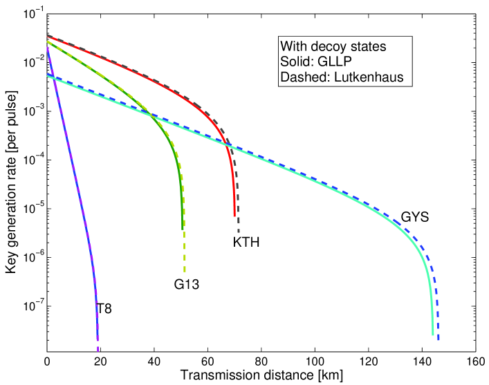
Figure 3: shows the relationship between key generation rate and the transmission distance for decoy state QKD, comparing Lütkenhaus and GLLP. The key parameters are listed in TABLE I. Using the Cascade protocol [30], the error correction efficiency is 1.16. Here we assume the efficiency of privacy amplification is 1. Details of QKD simulations can be seen in [25].

For comparison, we list the QBERs of four GLLP curves at maximal distance in Fig. 3 are $5.19\%$, $4.21\%$, $5.11\%$ and $6.8\%$. We can see that these four values are close to those given by Fig. 2 of non-decoy state QKD. This is because stronger signals are allowed to use when decoy states are implemented, and then the QBER drops down, which cancels out the increase of QBER by higher channel loss.

Based on the simulation results of four QKD setups, we find that there is little to gain by restricting the security analysis to individual attacks, given that the two schemes—Lütkenhaus vs. GLLP—provide very close performances. In other words, our view is that one is better off considering unconditional security, rather than restricting to individual attacks.

III-D One example

Decoy state QKD experiments has recently been performed [26, 27, 28, 29]. We analyze a decoy state QKD experiment over 60km fiber experiment [27] as an example here. All raw experiment data are listed in TABLE II.

Distance	$\lambda$	$N$	$N_{vac}$	$K_{vac}$
$60km$	$1550nm$	$104.8Mb$	$16.63Mb$	$1033b$
$\mu$	$N_{\mu}$	$N_{\mu}^{s}$	$K_{\mu}^{s}$	$K_{\mu}^{err}$
$0.55$	$66.86Mb$	$33.40Mb$	$60.50kb$	$1845b$
$\nu$	$N_{\nu}$	$N_{\nu}^{s}$	$K_{\nu}^{s}$	$K_{\nu}^{err}$
$0.152$	$21.34Mb$	$10.69Mb$	$5397b$	$455b$

TABLE II: Raw QKD experiment parameters from [27]. The unit $b$ stands for bit.

From TABLE II, we can calculate the key parameters for security analysis, listed in TABLE III. The definitions are given in Section II.

$q$	$Q_{\mu}$	$E_{\mu}$	$Y_{0}=Q_{vac}$	$Q_{\nu}$
$0.319$	$1.81\times 10^{-3}$	$3.05\%$	$1.11\times 10^{-4}$	$5.47\times 10^{-4}$

TABLE III: Key parameters for the security analysis of [27] derived from TABLE II.

Now, we can apply the data post-processing for decoy state QKD. We can estimate $Q_{1}$ by Eq. (6). For $e_{1}$ we use a different formula

$$e_{1} \leq\frac{E_{\mu}Q_{\mu}e^{\mu}-e_{0}Y_{0}}{Q_{1}e^{\mu}}.$$ (7)

The reason is that in the real experiment [27], $e_{1}$ of decoy states deviates largely from that of signal states. The deviation is caused by the imperfections of attenuators. Thus, we use the QBER of signal states $E_{\mu}$ to estimate $e_{1}$. It reminds us the key assumption of decoy state QKD: all $Y_{i}$ and $e_{i}$ are the same in the signal states and in the decoy states [22].

Substituting parameters of TABLE III into Eqs. (6) and (7), we get $Q_{1}\geq 8.50\times 10^{-4}$ and $e_{1}\leq 2.73\%$. Then we apply the Cascade error correction scheme [30], sacrificing a fraction of $1.16H_{2}(E_{\mu})=0.486$ of the sifted key, where $1.16$ is the error correction efficiency. Then from Eqs. (3) and (4), we get the key generation rate $R_{Lutkenhaus}=9.98\times 10^{-5}$ and $R_{GLLP}=9.04\times 10^{-5}$ . We randomly choose parities and obtain a final key with length of $K_{Lutkenhaus}=NR_{Lutkenhaus}=10.5kbit$ and $K_{GLLP}=NR_{GLLP}=9.47kbit$ . We can see the difference between the key lengths of GLLP and Lütkenhaus is within 10%. For the case of considering statistical fluctuations, one can refer to [27].

IV Conclusion

In this paper, we compare the security analysis of Lütkenhaus, against individual attack, and Gottesman-Lo-Lütkenhaus-Preskill, general security analysis. Our simulation results show that these two schemes provide close performances. Thus, we conclude that one is better off considering unconditional security, rather than restricting to individual attacks. In the security analysis, we emphasize that the QBER is not the only criterion of security due to the imperfections of QKD setups.

V Acknowledgments

This work is mostly from Xiongfeng Ma’s Master Thesis (see ArXiv: quant-ph/0503057) under the supervision of Hoi-Kwong Lo at University of Toronto. We thank Chi-Hang Fred Fung, N. Lütkenhaus, Bing Qi and Yi Zhao for enlightening discussions. Financial support from University of Toronto, CFI, CIAR, CIPI, Connaught, CRC, NSERC, OIT, PREA and Chinese Government Award for Outstanding Self-financed Students Abroad is gratefully acknowledged.

References

- [1] C. H. Bennett and G. Brassard, “Quantum cryptography: Public key distribution and coin tossing,” in Proceedings of IEEE International Conference on Computers, Systems, and Signal Processing, (Bangalore, India), pp. 175–179, IEEE, New York, 1984.
- [2] A. K. Ekert, “Quantum cryptography based on bell’s theorem,” Physical Review Letters, vol. 67, p. 661, 1991.
- [3] D. Mayers, “Unconditional security in quantum cryptography,” Journal of the ACM, vol. 48, p. 351 406, May 2001.
- [4] H.-K. Lo and H.-F. Chau, “Unconditional security of quantum key distribution over arbitrarily long distances,” Science, vol. 283, p. 2050, 1999.
- [5] P. W. Shor and J. Preskill, “Simple proof of security of the BB84 quantum key distribution protocol,” Physical Review Letters, vol. 85, p. 441, July 200.
- [6] N. Gisin, G. Ribordy, W. Tittel, and H. Zbinden, “Quantum cryptography,” REVIEWS OF MODERN PHYSICS, vol. 74, pp. 145–195, JANUARY 2002.
- [7] A. Y. Dominic Mayers, “Quantum cryptography with imperfect apparatus,” FOCS, 39th Annual Symposium on Foundations of Computer Science, p. 503, 1998.
- [8] N. Lütkenhaus, “Security against individual attacks for realistic quantum key distribution,” Physical Review A, vol. 61, p. 052304, 2000.
- [9] G. Brassard, N. Lütkenhaus, T. Mor, and B. Sanders, “Security aspects of practical quantum cryptography,” Physical Review Letters, vol. 85, p. 1330, 2000.
- [10] S. Félix, N. Gisin, A. ’e Stefanov, and H. Zbinden, “Faint laser quantum key distribution: eavesdropping exploiting multiphoton pulses,” Journal of Modern Optics, vol. 48, no. 13, p. 2009, 2001.
- [11] H. Inamori, N. Lütkenhaus, and D. Mayers, “Unconditional security of practical quantum key distribution,” quant-ph/0107017, 2001.
- [12] M. Koashi and J. Preskill, “Secure quantum key distribution with an uncharacterized source,” Physical Review Letters, vol. 90, p. 057902, 2003.
- [13] D. Gottesman, H.-K. Lo, N. Lutkenhaus, and J. Preskill, “Security of quantum key distribution with imperfect devices,” Quantum Information and Computation, vol. 4, p. 325, 2004.
- [14] C. H. Bennett, F. Bessette, G. Brassard, L. Salvail, and J. A. Smolin, “Experimental quantum cryptography,” Journal of Cryptology, vol. 5, no. 1, pp. 3–28, 1992.
- [15] P. D. Townsend, “Experimental investigation of the performance limits for first telecommunications-window quantum cryptography systems,” IEEE Photonics Technology Letters, vol. 10, pp. 1048–1050, July 1998.
- [16] G. Ribordy, J.-D. Gautier, N. Gisin, O. Guinnard, and H. Zbinden, “Automated ”plug & play” quantum key distribution,” Electronics Letters, vol. 34, no. 22, pp. 2116–2117, 1998.
- [17] M. Bourennane, F. Gibson, A. Karlsson, A. Hening, P. Jonsson, T. Tsegaye, D. Ljunggren, and E. Sundberg, “Experiments on long wavelength (1550nm) ”plug and play” quantum cryptography systems,” Optical Society of America, vol. 4, pp. 383–387, May 1999.
- [18] C. Gobby, Z. L. Yuan, and A. J. Shields, “Quantum key distribution over 122 km of standard telecom fiber,” Applied Physics Letters, vol. 84, pp. 3762–3764, 2004.
- [19] B. Huttner, N. Imoto, N. Gisin, and T. Mor, “Quantum cryptography with coherent states,” Physical Review A, vol. 51, p. 1863, 1995.
- [20] N. Lütkenhaus and M. Jahma, “Quantum key distribution with realistic states: photon-number statistics in the photon-number splitting attack,” New Journal of Physics, vol. 4, pp. 44.1–44.9, 2002.
- [21] W.-Y. Hwang, “Quantum key distribution with high loss: Toward global secure communication,” Physical Review Letters, vol. 91, p. 057901, August 2003.
- [22] H.-K. Lo, X. Ma, and K. Chen, “Decoy state quantum key distribution,” Physical Review Letters, vol. 94, p. 230504, June 2005.
- [23] X.-B. Wang, “Beating the pns attack in practical quantum cryptography,” Physical Review Letters, vol. 94, p. 230503, 2005.
- [24] J. W. Harrington, J. M. Ettinger, R. J. Hughes, and J. E. Nordholt, “Enhancing practical security of quantum key distribution with a few decoy states,” ArXiv.org:quant-ph/0503002, 2005.
- [25] X. Ma, B. Qi, Y. Zhao, and H.-K. Lo, “Practical decoy state for quantum key distribution,” Physical Review A, vol. 72, p. 012326, July 2005.
- [26] Y. Zhao, B. Qi, X. Ma, H.-K. Lo, and L. Qian, “Experimental quantum key distribution with decoy states,” Physical Review Letters, vol. 96, p. 070502, FEBRUARY 2006.
- [27] Y. Zhao, B. Qi, X. Ma, H.-K. Lo, and L. Qian, “Simulation and implementation of decoy state quantum key distribution over 60km telecom fiber,” ArXiv: quant-ph/0601168, 2006.
- [28] C.-Z. Peng, J. Zhang, D. Yang, W.-B. Gao, H.-X. Ma, H. Yin, H.-P. Zeng, T. Yang, X.-B. Wang, and J.-W. Pan, “Experimental long-distance decoy-state quantum key distribution based on polarization encoding,” ArXiv:quant-ph/0607129, 2006.
- [29] P. A. Hiskett, D. Rosenberg, C. G. Peterson, R. J. Hughes, S. Nam, A. E. Lita, A. J. Miller, and J. E. Nordholt, “Long-distance quantum key distribution in optical fiber,” ArXiv.org:quant-ph/0607177, 2006.
- [30] G. Brassard and L. Salvail, “Secret-key reconciliation by public discussion,” Advances in Cryptology EUROCRYPT ’93, May 1993.
- [31] H.-K. Lo and J. Preskill, “Phase randomization improves the security of quantum key distribution,” ArXiv: quant-ph/0504209, 2005.
- [32] V. Scarani, G. R. A. Acin, and N. Gisin, “Quantum cryptography protocols robust against photon number splitting attacks for weak laser pulse implementations,” Physical Review Letters, vol. 92, p. 057901, 2004.
- [33] K. Tamaki and H.-K. Lo, “Unconditionally secure key distillation from multiphotons,” Physical Review A, vol. 73, p. 010302, 2006.