Nearest neighbour spacing distribution of basis in some intron-less and intron-containing DNA sequences

Abstract

We show that the nearest neighbour distribution of distances between basis pairs of some intron-less and intron-containing coding regions are the same when a procedure, called unfolding, is applied. Such a procedure consists in separating the secular variations from the oscillatory terms. The form of the distribution obtained is quite similar to that of a random, i.e. Poissonian, sequence. This is done for the HUMBMYH7CD, DROMYONMA, HUMBMYH7 and DROMHC sequences. The first two correspond to highly coding regions while the last two correspond to non-coding regions. We also show that the distributions before the unfolding procedure depend on the secular part but, after the unfolding procedure we obtain an striking result: all distributions are similar to each other. The result becomes independent of the content of introns or the species we have chosen. This is in contradiction with the results obtained with the detrended fluctuation analysis in which the correlations yield different results for intron-less and intron-containing regions.

1 Introduction

In recent times DNA of new species have been sequenced, opening new questions in biological physics. Large data of genomic sequences are now available and ready to be analyzed. In particular, the study of their statistical properties is of broad interest. Up to now, several works addressed the correlations in coding and non-coding regions [1, 2]. Many statistical measures have been introduced since those works appeared: the detrended fluctuation analysis [3], diffusion entropy analysis [4], factorial moment analysis [5], wavelet analysis [6], among others.

Despite several efforts (see Ref. [5] and references therein), the question about the statistical properties between intron-less and intron-containing coding regions is still open. Here we use two complementary techniques to study the “short-range” statistical properties of DNA sequences. Our work considers, at this stage, only monoplets, but studies on duplets and triples are in progress  [12]. First we use a generalized detrended fluctuation analysis, commonly called unfolding [7, 8, 9], to separate the secular trend and the non-secular properties of the sequences. Then, the nearest neighbour distribution is obtained and analyzed.

In the next section we define the cumulative basis density and the mathematical procedure called unfolding. The cumulative basis density is obtained for: two intron-less sequences (0% of introns), HUMBMYH7CD and DROMYONMA, corresponding to the Human $\beta$-cardiac myosin heavy chain (MHC) and Drosophila melanogaster MHC, respectively; and two intron-containing coding sequences, HUMBMYH7 and DROMHC that correspond to the Human $\beta$-cardiac MHC and to the Drosophila melanogaster MHC, respectively. The sequences were taken mainly from GenBank[13] and were analyzed with the detrended fluctuation analysis [2]. The number of introns of each sequence is given in Table 1. In section 3 the nearest neigbour distribution is obtained yielding a universal feature. Examples of the nonsense results obtained without a proper unfolding procedure are also given there. A brief conclusion follows.

code	size	introns	basis-content (%)				$\langle s\rangle$ (basis)
	(basis)	(%)	A	T	C	G	A	T	C	G
HUMBMYH7CD	5999	0	26.7	16.0	26.0	31.3	3.7	6.3	3.8	3.2
DROMYONMA	6338	0	24.1	14.5	18.7	21.7	3.3	5.4	4.2	3.6
HUMBMYH7	28438	73	23.6	23.0	27.4	26.0	4.2	4.4	3.6	3.9
DROMHC	22663	72	30.6	18.4	23.6	27.5	3.3	5.5	4.3	3.7

Table 1: Some statistical properties of the sequences analyzed here. A, T, C, and G correspond to adenine, thymine, cytosine and guanine, respectively. $\langle s\rangle$ stands for the mean level spacing of each basis and is calculated as an arithmetic average.

2 Unfolding procedure

Following Ref. [5] we define the density of basis as

$$\rho^{\beta}(x)=\sum_{i=1}^{N_{\beta}}\delta(x-x_{i}^{\beta})$$ (1)

where $\{x_{i}^{\beta}\}_{i=1}^{N_{\beta}}$ is the ordered set of $N_{\beta}$ positions of the basis. Here $\beta$ stands for adenine (A), thymine (T), cytosine (C), or guanine (G) in DNA. In the last equation $\delta(x)$ is the Dirac $\delta$-function. The cumulative basis density or staircase function is defined as the derivative of $\rho^{\beta}(x)$:

$$\mathrm{N}^{\beta}(x)=\sum_{i=1}^{N_{\beta}}\Theta(x-x_{i}^{\beta}),$$ (2)

where $\Theta(x)$ is the Heaviside function. This function is plotted in Fig. 1 for the sequences HUMBMYH7CD, DROMYONMA, HUMBMYH7 and DROMHC. Notice that this quantity corresponds to the inverse function of the cumulative position plots of Ref. [10].

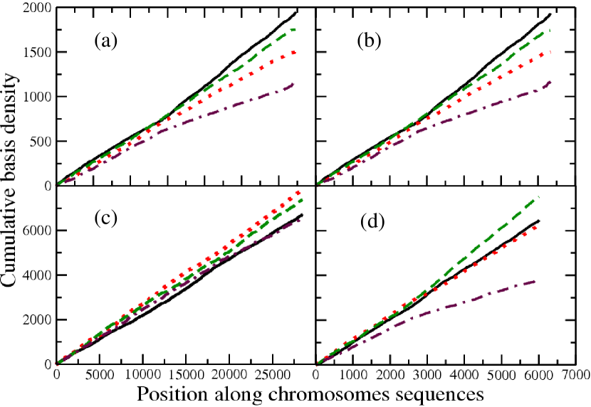
Figure 1: (color online) Cumulative basis density of the sequences (a) DROMYONMA, (b) DROMHC, (c) HUMBMYH7CD and (d) HUMBMYH7 . The first column corresponds to non coding region and the second one to coding one. The first row corresponds to D. melanogaster and the second one to human. The solid (black) line corresponds to adenine (A), the dash-dotted (maroon) line to thymine (T), the dotted (red) line to cytosine (C) and the dashed line (green) to guanine (G).

Following Refs. [7, 8, 9], the cumulative basis density can be expressed as

$$\mathrm{N}^{\beta}(x)=\langle\mathrm{N}^{\beta}(x)\rangle+\mathrm{N}_{osc}^{\beta}(x),$$ (3)

where $\langle\mathrm{N}^{\beta}(x)\rangle$ is a mean or secular part and $\mathrm{N}_{osc}^{\beta}(x)$ is the oscillating one. The brackets in the secular part refer to average in position. Notice that the secular part is a function of $x$ and is not necessarily smooth. In quantum physical systems, for instance, $\langle\mathrm{N}^{\beta}(x)\rangle$ contains the periodic orbit information, ı.e. the classical one [9]. As seen in Fig. 1, cumulative densities of different basis and/or sequences have different secular parts. Some look almost linear while other appear linear by parts. It is not clear for us the biological origin of the abrupt change in the slope of $\langle\mathrm{N}^{\beta}(x)\rangle$. However, for bacterial genomes, similar changes in density corresponds to the replication origin [10]. Analytical expressions for the secular part are unknown up to now, hence we will use some of the numerical methods commonly used in spectral statistics. For instance, we will use a polynomial fitting. The degree of the polynomial is chosen, as usual, as the minimum in which the fluctuations does not change anymore. Notice that this unfolding procedure is more general that the detrended fluctuation analysis, since the latter uses only a linear fitting. A systematical study and a comparison with a different unfolding procedure (window analysis) will be given elsewhere [12]. In the sequences of Table 1 we tested fittings with polynomials from 8th until 18th degree. We also used windows from 100 to 1000 distances. Within this range of parameters (polynomial degree and window) the results we present are stationary, i.e. the results do not change.

The transformation that allows the comparison of the fluctuations for systems with different secular parts is the unfolding. It works as follows. Lets define a new unfolded sequence $\{y_{i}^{\beta}\}_{i=1}^{N_{\beta}}$ where

$$y_{i}^{\beta}=\langle\mathrm{N}^{\beta}(x_{i}^{\beta})\rangle.$$ (4)

With this transformation the new sequence has a uniform density and mean level spacing equal to unity, i.e. $\langle y_{i+1}^{\beta}-y_{i}^{\beta}\rangle=1$.

3 Nearest neigbour spacing distribution

The nearest neigbour spacing distribution, $p(s)$, is the observable most commonly used to study the “short-range” fluctuations in the density of basis. Here $s_{i}^{\beta}=y_{i+1}^{\beta}-y_{i}^{\beta}$. The quotes mean that the short range is defined in units of the mean level spacing $\langle s^{\beta}\rangle$. Then, for a very diluted basis in a sequence, $p(s)$ refers to very long distances in the complete sequence and vice versa. The distribution $p(s)$ then yields the probability density to have two neigbouring levels $y_{i}^{\beta}$ and $y_{i+1}^{\beta}$ at a spacing $s$. With the unfolding procedure the function $p(s)$ and its first moment are normalized to unity. The mean level spacing $\langle s\rangle$ on basis, without unfolding, is given in Table 1. Notice that this is not a well defined quantity for some sequences like thymine in DROMYONMA (dash-dotted in Fig. 1), since it has two different values and hence, the unfolding procedure is required.

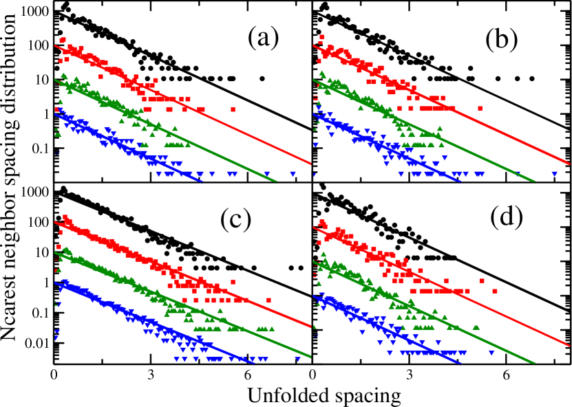
Figure 2: (color online) Nearest neigbour spacing distribution, $p(s)$, for the same sequences of Fig. 1 and following the same order. The circles (black) correspond to the $p(s)\times 1000$ of adenine, the squares (red) to the $p(s)\times 100$ of cytosine, the triangles up to the $p(s)\times 10$ of guanine and the triangles down (blue) to the $p(s)$ of thymine. The solid lines correspond to the Poissonian result $p(s)=\exp(-x)$ times the corresponding scaling factor.

In Fig. 2 we show the obtained nearest neigbour spacing distribution $p(s)$ for the different basis for the different sequences. As seen in this figure, they are very similar to the uncorrelated Poissonian prediction

$$p(s)=exp(-s).$$ (5)

The main differences between the results of the genomic sequences and the Poissonian prediction appear at both, very short and very long distances. The explanation at short distances is trivial: they are related to the physical size of the basis which avoid distances smaller than the physical size of a basis. This generates a “repulsion hole”. The repulsion hole is not due to the unfolding procedure but this procedure makes the hole much more evident. The result we get in 2 is opposite to the well-known result given in [3]. This means that, at least in the sequences we used, it is impossible to differentiate coding and non-coding regions with statistical analysis. Biological information is present only in the secular part but not in the fluctuations.

Now we will show some results without the unfolding procedure. In Fig. 3 we show the histograms we obtained for thymine in the four sequences. They are no normalized nor unfolded. As seen, some of them, Fig. 3 (a) and (c), are very similar to the Poissonian prediction while other, Fig. 3 (b) and (d), are quite different. This behavior give the impression that statistical distribution for non coding and coding regions are different. However this wrong conclusion is due to an artifact because in Fig. 2 they have clearly the same distribution. The explanation of this behavior is very simple: since the density is not uniform and it depends on the position along the sequences, the distances between basis have different statistical weights. Missing or incorrect rectification (unfolding), gives place to an incorrect measurement of the fluctuations and to possible wrong conclusions. Then, the unfolding procedure eliminates artifacts due to a wrong average. To find the correct way to unfold a sequence is a very delicate and difficult task [9]. However, it is the way to obtain a measure of the fluctuations which allow us a comparison between systems having different trends.

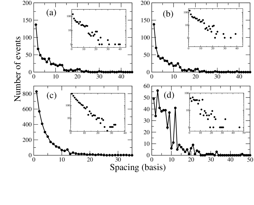
Figure 3: Nearest neigbour spacing histograms for thymine in the same order as the previous figure. No normalization nor unfolding was performed. Notice that the fluctuation at small spacings are large in case (a) and (b) and huge in case (d). An exponential fitting in case (c) is correct however it is non-sense in case (d). The insets show the same plots with the Y-axis in logaritmic scale.

4 Conclusions

We introduced the cumulative basis density as well as the unfolding procedure to analyze distances between basis in genomic sequences. We have shown that the nearest neigbour spacing distribution is very close to the Poissonian distribution. The main differences between them have been found in short distances where the physical size of each basis generates a “repulsion hole”. The results we have got for the nearest neigbour spacing distribution are quite different that those available in the literature for other quantities like correlations. We obtained the same result, almost Poissonian, for two intron-less and two intron-containing coding sequences. This suggest that a proper unfolding procedure should be implemented before any statistical analysis of genomic sequences. Artifacts due to a wrong average could appear. Our results indicate strongly that statistical measures in genomic sequences without proper unfolding could give artifacts and probably several results in the literature on the area are not correct.

References

- [1] W. Li and W. Kaneko, Europhys. Lett. 17 (1992) 655.
- [2] C. K. Peng et al, Nature 356 (1992) 168.
- [3] C. K. Peng et al, Phys. Rev. E 49 (1994) 1685.
- [4] N. Scafetta, V. Latora, P. Grigolini, Phys. Lett. A 299 (2002) 565.
- [5] A. K. Mohanty, A. V. S. S. Narayana Rao, Phys. Rev. Lett. 84 (2000) 1832.
- [6] A. Arneodo, E. Bacry, P. V. Graves, J. F. Muzy Phys. Rev. Lett. 74 (1995) 3293.
- [7] M. L. Metha, Random Matrices, 2nd. ed., Academic, New York, 1991.
- [8] T. A. Brody et al, Rev. Mod. Phys. 53 (1981) 385.
- [9] T. Guhr, A. Müller-Groeling, H. A. Weidenmüller, Phys. Rep. 299 (1998) 189.
- [10] J. Sánchez, M. V. José, Biochem. Biophys. Res. Comm. 299 (2002) 126.
- [11] M. V. José, T. Govezensky, J. R. Bobadilla Physica A 351 (2005) 477.
- [12] M. F. Higareda, H. Hernández-Saldaña y R. A. Méndez-Sánchez, to be published.
- [13] http://www.ncbi.nlm.nih.gov/Genbank/index.html