Fast cooling of trapped ions using the dynamical Stark shift gate

Abstract

A laser cooling scheme for trapped ions is presented which is based on the fast dynamical Stark shift gate, described in [Jonathan et al., Phys. Rev. A62, 042307]. Since this cooling method does not contain an off resonant carrier transition, low final temperatures are achieved even in traveling wave light field. The proposed method may operate in either pulsed or continuous mode and is also suitable for ion traps using microwave addressing in strong magnetic field gradients.

Introduction – The ability to laser cool ions to within the vicinity of the motional ground state is a key factor in the realization of efficient quantum computation Wineland et al. (1998a). Various cooling schemes have been suggested and implemented, achieving lower and lower temperature and increased cooling rates. The schemes range from the simplest Doppler cooling Wineland and Dehmelt (1975); Hansch and Schawlow (1975) to more sophisticated ion trap cooling methods, including sideband cooling for two level atoms Diedrich et al. (1989); Wineland and Dehmelt (1975); Wineland et al. (1978), Raman side band cooling Monroe et al. (1995) which may be used for ions and for atomsHamann et al. (1998); Vuletic et al. (1998) and cooling schemes based on electromagnetically induced transparency (EIT) Eschner and Keitel (2000). The existing schemes may be divided into pulsed schemes Monroe et al. (1995) and continuous schemes.

The two-level and Raman sideband cooling schemes employ Rabi frequencies that are typically an order of magnitude lower than the trap frequency. This is necessary to avoid off-resonant excitations which increase the average phonons number $\langle n\rangle$ and thus lead to heating. Hence, these off-resonant excitations increase the final temperature of the scheme. To overcome this limit, a scheme that employs EIT was introduced in Eschner and Keitel (2000) and demonstrated in Roos et al. (2000). This scheme uses interference to cancel the undesirable off-resonant carrier transition by suppression of absorption. This scheme can achieve low temperatures as well as high cooling rates, but the exact calibration of the laser intensity and the high intensities which are needed, makes the scheme challenging.

In this work we present an alternative approach to this problem that relies on the fast Stark shift gate Jonathan et al. (2000); Jonathan and Plenio (2001). In this scheme off-resonant carrier transitions that would lead to heating are forbidden even when operating in the traveling wave regime at Rabi frequencies that are of the order of the trap frequency. The higher Rabi-frequency and the cancelation of the carrier transition promises increased cooling rates and lower final temperatures. This advantage applies both for the pulsed scheme and the continuous cooling schemes. It is important to note that unlike the original Stark shift gate which requires careful intensity stabilization to achieve high fidelity Jonathan et al. (2000); Jonathan and Plenio (2001) the Stark shift cooling method is only weakly affected by laser intensity fluctuations. Our scheme is applicable for trapped ions or atoms and is also suitable for an ion trap scheme employing microwave addressing method in strong magnetic field gradients as proposed in Mintert and Wunderlich (2001). The presented scheme satisfies the dark state conditionDum et al. (1994), i.e. the ions are pumped into a zero-phonon state that no longer interact with the the applied laser fields.

This paper is organized as follows, We first describe the operation of the Stark shift gate and then explain the idea of using this gate for cooling both in pulsed and continuous operation. To analyze our proposed scheme we deduce the rate equation in the Lamb-Dicke limit and verify the predictions thus obtained with exact numerical simulations. In order to discuss the efficiency of the method we compare the proposed cooling scheme with previously proposed cooling schemes. In order to demonstrate the applicability of the scheme to chains of ions we present numerical results for the simultaneous cooling of three ions. We finish with a discussion and conclusion.

The Stark-shift gate – In the following we briefly explain the basic mechanism underlying the Stark shift gate Jonathan et al. (2000); Jonathan and Plenio (2001). The Hamilton operator of a single ion driven by a traveling-wave laser field of Rabi frequency $\Omega$ in the standard interaction picture with respect to the free atom and phonons is given by

$$H=\Omega\{\sigma_{+}\exp(i\eta[ae^{-i\nu t}+a^{\dagger}e^{i\nu t}]-i\delta t)+H.c\},$$

where $\hbar=1$, $\delta$ is the laser atom detuning, $\nu$ the trap frequency and $\eta$ is the Lamb-Dicke parameter Wineland et al. (1998b). For $\delta=0$ and employing $\eta\ll 1$, the exponent may be expanded to first order in $\eta$ yielding $H\cong\Omega(\sigma_{x}+\eta\sigma_{y}(ae^{-i\nu t}+a^{\dagger}e^{i\nu t}))$. In a further interaction picture with respect to $H_{0}=\Omega\sigma_{x}$, we obtain $H_{I}=i\eta\Omega^{\prime}[e^{i(2\Omega-\nu)t}\sigma_{+}a+e^{i(2\Omega+\nu)t}\sigma_{+}a^{\dagger}]+H.c.$ where $\sigma_{+}=|+\rangle\langle-|$. Setting $\Omega=\frac{\nu}{2}$ (see also Lizuain and Muga (2006); Jonathan et al. (2000); Jonathan and Plenio (2001)) and neglecting off resonant terms we obtain

$$H_{ss}=\frac{i\eta\nu}{2}[\sigma_{+}a-\sigma_{-}a^{\dagger}].$$ (1)

Careful numerical investigations demonstrate that $H_{ss}$ represents an excellent approximation to the exact dynamics Jonathan et al. (2000); Jonathan and Plenio (2001). It is of particular importance to note that the Stark-shift gate does not have off-resonant carrier transitions, despite being operated in the traveling wave regime, making it a very accurate and fast quantum gate. As the carrier transition represents the dominant heating term in laser cooling, this cancellation of the carrier transition suggests the use of the Stark shift gate for fast laser cooling. The Stark shift gate requires stabilization of the Rabi frequency at $\Omega=\frac{\nu}{2}$. However, in laser cooling we are only interested in the preparation of a target state – the ground state. This suggests that the constraints on the stability of the Rabi frequency are much less severe in the application of the Stark shift gate to laser cooling than for its gate operation. The verification and exploitation of this idea is the purpose of the remainder of this work.

Stark-shift gate cooling – In the following we will describe how the Stark shift gate may be used to implement both pulsed and continuous laser cooling schemes. We begin with the pulsed scheme as this clarifies the origin of the speed advantage in both schemes. We proceed in close analogy to the pulsed scheme based on the regular gate Monroe et al. (1995). Assume that the system starts in state $|\downarrow\rangle|n\rangle$. First a resonant laser pulse implements $|\downarrow\rangle|n\rangle\rightarrow|-\rangle|n\rangle$. Then the Stark shift gate creates the rotation $\left|-\right\rangle\left|n\right\rangle\rightarrow\left|+\right\rangle\left|n-1\right\rangle$. A resonant pulse then implements $\left|+\right\rangle\left|n-1\right\rangle\rightarrow\left|\uparrow\right\rangle\left|n-1\right\rangle$ hence moving the system to a dissipative level. Spontaneous decay predominantly leads to $\left|\uparrow\right\rangle\left|n-1\right\rangle\rightarrow\left|\downarrow\right\rangle\left|n-1\right\rangle$ and the process as a whole leads to the net loss of one phonon. This set of pulses is repeated until the limiting temperature is achieved. This scheme yields lower final temperatures and is faster under ideal conditions than the usual sideband cooling. It is evident that the bottleneck of the scheme is the $\left|-\right\rangle\left|n\right\rangle\rightarrow\left|+\right\rangle\left|n-1\right\rangle$ and it is this process that is accelerated by the use of the Stark shift gate. The above scheme may also be implemented in the microwave regime Mintert and Wunderlich (2001) where instead of the cooling laser, a combination of a microwave and a steep magnetic field gradient is used and the coupling to the dissipative level is achieved by resonant lasers.

The continuous scheme is most efficiently implemented in a three level configuration as shown in Fig. 1. The Hamiltonian of this system is given by

$$H = \omega_{1}\left|g_{1}\right\rangle\left\langle g_{1}\right|+\omega_{2}\left|g_{2}\right\rangle\left\langle g_{2}\right|+\omega_{3}\left|e\right\rangle\left\langle e\right|+\nu a^{\dagger}a$$ (2)

$$- \Omega\left(\left|g_{1}\right\rangle\left\langle e\right|e^{-i(\omega_{1}+\Delta)t}+\left|g_{2}\right\rangle\left\langle e\right|e^{-i(\omega_{2}+\Delta)t}+H.c\right)$$

$$- \Omega_{c}\left(\left|g_{1}\right\rangle\left\langle g_{2}\right|e^{i(k_{c}x-\omega_{c}t)}+H.c\right).$$

\psfrag{e}{$\left|e\right\rangle$}\psfrag{o}{$\Omega$}\psfrag{oc}{$\Omega_{c}$}\psfrag{g1}{$\left|g_{2}\right\rangle$}\psfrag{g2}{$\left|g_{1}\right\rangle$}\psfrag{-0}{$\left|-,0\right\rangle$}\psfrag{-1}{$\left|-,1\right\rangle$}\psfrag{-2}{$\left|-,2\right\rangle$}\psfrag{+0}{$\left|+,0\right\rangle$}\psfrag{+1}{$\left|+,1\right\rangle$}\psfrag{+2}{$\left|+,2\right\rangle$}\psfrag{e0}{$\left|e,0\right\rangle$}\psfrag{e1}{$\left|e,1\right\rangle$}\psfrag{e2}{$\left|e,2\right\rangle$}\includegraphics[width=173.44534pt,height=101.17645pt]{tr}

Figure 1: The required atomic level structure is given in the left upper corner. A cooling Laser $\Omega_{c}$ manifests the Stark shift gate, creating a rotation $\left|-\right\rangle\left|n\right\rangle\leftrightarrow\left|+\right\rangle\left|n-1\right\rangle$. The $\Omega_{1}$ and $\Omega_{2}$ Lasers couple only the $\left|+\right\rangle$ state to the dissipative level and leave the $\left|-\right\rangle$ state decoupled. The cooling process is schematically depicted in the lower right part of the picture.

The laser on the meta-stable $|g_{1}\rangle\leftrightarrow|g_{2}\rangle$ transition is used to implement the Stark shift gate by tuning its Rabi frequency to the resonance condition $\Omega_{c}=\frac{\nu}{2}$. This implements the rotation $\left|-\right\rangle\left|n\right\rangle\rightarrow\left|+\right\rangle\left|n-1\right\rangle$. The two lasers on the $|g_{i}\rangle\leftrightarrow|e\rangle$ transition are chosen to have equal Rabi frequency and detuning and thus couple the $\left|+\right\rangle=\frac{1}{\sqrt{2}}(|g_{1}\rangle+|g_{2}\rangle)$ state to the dissipative level $\left|e\right\rangle$ with spontaneous decay rates $2\Gamma_{1}$ and $2\Gamma_{2}$ to the states $\left|g_{1}\right\rangle$,$\left|g_{2}\right\rangle$ respectively. The two lasers leave the state $\left|-\right\rangle$ decoupled from the dissipative level. It is important to note that the lasers on the $|g_{i}\rangle\leftrightarrow|e\rangle$ do not couple the internal and the phonon degrees of freedom, i.e, their Lamb-Dicke parameter should be made as small as possible by adjusting the angle between the laser and the ion trap.

The basic cooling cycle in the continuous scheme works as follows. The laser with Rabi frequency $\Omega_{c}$ creates the rotation $\left|-\right\rangle\left|n\right\rangle\leftrightarrow\left|+\right\rangle\left|n-1\right\rangle$ based on the Stark shift gate. The lasers couple the $\left|+\right\rangle\left|n-1\right\rangle$ state to the dissipative level $|e\rangle\left|n-1\right\rangle$, which dissipates back to one of the $\left|g_{i},n-1\right\rangle$’s which are superpositions of $\left|+\right\rangle\left|n-1\right\rangle$ and $\left|-\right\rangle\left|n-1\right\rangle$. If the decay is to the $\left|-\right\rangle\left|n-1\right\rangle$, one phonon has been lost and cooling is achieved, whereas if the decay is to the $\left|+\right\rangle\left|n-1\right\rangle$ state the cycle is repeated. Thus on average phonons are dissipated out of the system. Note that this mechanism is independent of the sign of the detuning $\Delta$.

Analytical Results – Following the heuristic arguments presented so far we will now derive analytic expressions for the cooling rate and final temperature of our scheme based on a Master equation approach. The dynamics and the final state can be obtained from the master equation,

$$\frac{\partial}{\partial t}\rho=\frac{1}{i}[H,\rho]+\mathcal{L}\rho,$$ (3)

where $H$ is the Hamiltonian eq. (2) and $\mathcal{L}$ is the Liouville operator describing the dissipative channels of from level $|e\rangle$ to $|g_{i}\rangle$. In the following we use the techniques presented in Lindberg and Javanainen (1986); Cirac et al. (1992). In this formalism, the equation of motion for the phonons is obtained by adiabatic elimination of the internal degrees of freedom of the ions. The final temperature and the cooling rate are obtained by expanding the Liouville operator and the density matrix in eq. (3) in the Lamb-Dicke parameter $\mathcal{L}=\mathcal{L}_{0}+\eta\mathcal{L}_{1}+\eta^{2}\mathcal{L}_{2}+\mathcal{O}(\eta^{3})$, $\rho=\rho_{0}+\eta\rho_{1}+\eta^{2}\rho_{2}+\mathcal{O}(\eta^{3})$. Inserting this into eq. (3) results in three equations, each for a different power of the Lamb-Dicke parameter as in Lindberg and Javanainen (1986). From these three equations the final temperature and the cooling rate are calculated. The validity of the expansion in the Lamb-Dicke parameter at the point $\Omega_{c}=\frac{\nu}{2}$ is restricted by the three conditions $\Gamma\nu\eta,\nu^{2}\eta,\Delta\nu\eta\ll\Omega^{2}$. The result of this approach is a rate equation for the phonon probability distribution $P(n)$ Javanainen et al. (1984)

$$\frac{d}{dt}P(n) = \eta^{2}\Big{(}A_{-}[(n+1)P(n+1)-nP(n)]$$ (4)

$$\hskip 17.07182pt+A_{+}[nP(n-1)-(n+1)P(n)]\Big{)}$$

where

$$A_{-}(\nu)\!=\!\frac{2\Gamma\Omega^{2}\Omega_{c}^{2}}{\Gamma^{2}(\nu-2\Omega_{c})^{2}+\left(2\Omega^{2}+(\nu-2\Omega_{c})(\Delta-\nu+\Omega_{c})\right)^{2}}$$ (5)

and $A_{+}=A_{-}(-\nu)$. From these expressions the final population and the rate are deduced to be

$$\langle n\rangle\!\!\! = \!\!\frac{A_{+}}{A_{-}-A_{+}}$$

$$=\!\frac{\Gamma^{2}(\nu-2\Omega_{c})^{2}+\left(2\Omega^{2}+(\nu-2\Omega_{c})(\Delta-\nu+\Omega_{c})\right)^{2}}{4\nu\left(2\Omega_{c}\Gamma^{2}+(\Delta+3\Omega_{c})\left(\nu^{2}+2\left(\Omega_{c}(\Delta+\Omega_{c})-\Omega^{2}\right)\right)\right)}$$

$$W\!\!\! = \!\!\eta^{2}(A_{-}-A_{+}),$$ (7)

where $W$ is the cooling rate. Numerics shown in Fig. 3 confirms that the $\langle n\rangle$ is minimized at the Stark shift gate point $\Omega_{c}\approx\frac{\nu}{2}$. At $\Omega_{c}=\frac{\nu}{2}$ we find $W=\frac{1}{8}\Gamma\eta^{2}\nu^{2}\Omega^{2}(\Omega^{-4}-4[4\Gamma^{2}\nu^{2}+(3\nu^{2}+2\Delta\nu-2\Omega^{2})^{2}]^{-1})$. The choice $\frac{\Gamma\nu}{\Omega^{2}}\eta=1$ realizes a cooling scheme with a rate $W=\frac{1}{8}\eta\Omega_{c}$ which is close to the inverse of the gate time $T=\frac{\pi}{\eta\Omega_{c}}$. Note that this choice saturates the conditions of validity in the above derivation, If one of the other conditions is saturated as well the final population is smaller by the factor of 2, which means that the choice $\Delta=\Gamma$ is optimal. Nevertheless, numerical results shown in Fig. 2 corroborate that the cooling time is of the order of the gate time.

\psfrag{W}{W}\psfrag{e}{$\eta$}\includegraphics[width=195.12767pt,height=101.17645pt]{RateDicke.eps}

Figure 2: The Rate at the optimal point. The squares are $\frac{1}{T_{C}}$, when $T_{C}$ is the time that takes to reduce the population from $\langle n\rangle=1$ to $\langle n\rangle=0.01$. The blue line corresponds to half a period of a Rabi frequency and the green line to the cooling rate calculated from the rate equations $W=\frac{1}{8}\eta\Omega_{c}$

\psfrag{o}{$\Omega_{c}$}\psfrag{n}{$\langle n\rangle$}\includegraphics[width=195.12767pt,height=101.17645pt]{AvgOmega.eps}

Figure 3: $\langle n\rangle$ as a function of $\Omega_{c}$. The minimum is at the Stark shift resonance. The continuous line is the rate equation result. The squares are calculated from a numerical solution of the Master equation for $\eta=1/20$ and the triangles are for $\eta=1/10$. In the limit $\eta\rightarrow 0$ The numerics coincide with the rate equations. The parameters are $\Gamma=10,\Omega=1/10,\nu=1$ and $\Delta=0$

Fig. 3 shows numerically and analytically that for the final $\langle n\rangle$ as a function of $\Omega_{c}$ we obtain a parabola with a minimum around the Stark shift resonance. At this point we find

$$\langle n\rangle=\frac{\Omega^{4}}{\nu\left(\nu\Gamma^{2}+\left(\Delta+\frac{3\nu}{2}\right)\left(\nu^{2}+2\left(\frac{1}{2}\left(\Delta+\frac{\nu}{2}\right)\nu-\Omega^{2}\right)\right)\right).}$$ (8)

Inserting the values of the optimum point, $\Gamma\nu\eta,\nu^{2}\eta,\Delta\nu\eta=\Omega^{2}$, yields a temperature proportional to $\eta^{2}$. For $\Omega=\nu/2$ heating $A_{+}$ is weaker than cooling $A_{-}$ whenever $\Omega^{2}\leq\frac{\nu\left(4\Gamma^{2}+4\Delta^{2}+9\nu^{2}+12\Delta\nu\right)}{4(2\Delta+3\nu)}$. The cooling efficiency is not strongly effected by the fluctuations of the laser. For example, at the optimal point, at $\eta=0.05$, for intensity fluctuations of 10 percent, the rate and the final temperature change by less then 50 percent.

Numerical results – The results deduced from the rate equations are correct in the limit $\eta\rightarrow 0$. In order to check the results for finite $\eta$ and see the dynamics, we compare these results to a numerical solution of the Master equation. In Fig. 3 a plot of the analytical final mean phonon number is compared to numerical results and as $\eta\rightarrow 0$ the rate equation results are reproduced. In order to compare the rates found for the final stages of cooling with the actual cooling time we reproduce the dynamics using Monte - Carlo simulation for the cooling of one phonon. Fig. 4 shows the dynamics of the mean phonon number.

\psfrag{na}{$\langle n\rangle$}\includegraphics[width=195.12767pt,height=101.17645pt]{Cooling2.eps}

Figure 4: $\langle n\rangle$ as a function of time using Monte Carlo simulation. The parameters used for the simulation: $\Delta=0$,$\Gamma=6$,$\nu=1$,$\Omega_{c}=1/2$,$\Omega_{1}=\Omega_{2}=1$,$\eta=1/10$. For these parameters the gate time is $\frac{\pi}{\eta\Omega}=62.5$. It could be seen from the numerics that the cooling time is in the same order of magnitude as the gate time.

The mean phonon number in sideband cooling is $\langle n\rangle=(\alpha+\frac{1}{4})\left(\frac{\Gamma}{\nu}\right)^{2}$ ,where $\alpha$ is a geometric factor of the order $1$ Stenholm (1986); Javanainen and Stenholm (1981). In order for sideband cooling to operate at the same rate as the proposed cooling, $\Gamma$ has to be of the order of $\nu/2\eta$ which means that the sidebands are not resolved, hence, sideband cooling could not be applied. The cooling rates and temperatures found in our scheme could be achieved by the EIT cooling method Eschner and Keitel (2000) but in this method the laser power should be at least an order of magnitude stronger then in the cooling described in this work.

Multi-mode cooling – Due to the cancelation of the carrier transition it suggests itself that our cooling method based on the Stark shift gate could be used to cool several modes simultaneously. Fig.5 shows Monte-Carlo simulation Plenio and Knight (1998) for the cooling of three modes in a three ion chain. Here we chose the laser Rabi frequency near the second mode frequency. The cooling rate achieved in this way of course slower than for a single ion, but still faster than side band cooling. In a different scheme individual ions could be addressed with lasers of different Rabi frequency each at the optimal working point for a different mode. Thus the whole chain could be cooled at times of the order the Stark shift gate time.

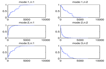
Figure 5: Monte-Carlo simulation for the cooling of three ions. The Rabi frequency is set to $\Omega_{c}=\frac{1}{2}\nu_{2}+0.15$. For three ions the frequencies are $\nu_{2}=\sqrt{3}\nu_{1},\nu_{3}=\sqrt{29/5}\nu_{1}$.

Conclusions – We have introduced a method for the fast cooling of an ion trap which operates with rates of the fast Stark shift gateJonathan et al. (2000). The final temperatures achieved are proportional to $\eta^{2}$(recoil energy). The cooling method is efficient both in continuous and pulsed operation, achieving lower temperatures and faster rates then ordinary sideband cooling. The gate is also suitable for ion traps with microwave frequency addressing Mintert and Wunderlich (2001).

Acknowledgements – We would like to thank H. Haeffner, N. Davidson and B. Reznik for helpful discussions. This work has been supported by the European Commission under the Integrated Project Qubit Applications (QAP) funded by the IST directorate as Contract Number 015848, the Royal Society and is part of the EPSRC QIP-IRC.

References

- Wineland et al. (1998a) D. J. Wineland, C. Monroe, W. M. Itano, D. Leibfried, B. E. King, and D. M. Meekhof, J. Res. Natl. Stand. Tech. 103, 259 (1998a).
- Wineland and Dehmelt (1975) D. Wineland and H. Dehmelt, Bull. Am. Phys. Soc 20, 637 (1975).
- Hansch and Schawlow (1975) T. Hansch and A. Schawlow, Opt. Commun 13, 68 (1975).
- Diedrich et al. (1989) F. Diedrich, J. C. Bergquist, W. M. Itano, and D. J. Wineland, Phys. Rev. Lett. 62, 403 (1989).
- Wineland et al. (1978) D. J. Wineland, R. E. Drullinger, and F. L. Walls, Phys. Rev. Lett. 40, 1639 (1978).
- Monroe et al. (1995) C. Monroe, D. M. Meekhof, B. E. King, S. R. Jefferts, W. M. Itano, D. J. Wineland, and P. Gould, Phys. Rev. Lett. 75, 4011 (1995).
- Hamann et al. (1998) S. E. Hamann, D. L. Haycock, G. Klose, P. H. Pax, I. H. Deutsch, and P. S. Jessen, Phys. Rev. Lett. 80, 4149 (1998).
- Vuletic et al. (1998) V. Vuletic , C. Chin, A. J. Kerman, and S. Chu, Phys. Rev. Lett. 81, 5768 (1998).
- Eschner and Keitel (2000) G. M. J. Eschner and C. H. Keitel, Phys. Rev. Lett. 85, 4458 (2000).
- Roos et al. (2000) C. F. Roos, D. Leibfried, A. Mundt, F. Schmidt-Kaler, J. Eschner, and R. Blatt, Phys. Rev. Lett. 85, 5547 (2000).
- Jonathan et al. (2000) D. Jonathan, M. B. Plenio, and P. L. Knight, Phys. Rev. A 62, 042307 (2000).
- Jonathan and Plenio (2001) D. Jonathan and M. B. Plenio, Phys. Rev. Lett. 87, 127901 (2001).
- Mintert and Wunderlich (2001) F. Mintert and C. Wunderlich, Phys. Rev. Lett. 87, 257904 (2001).
- Dum et al. (1994) R. Dum, P. Marte, T. Pellizzari, and P. Zoller, Phys. Rev. Lett. 73, 2829 (1994).
- Wineland et al. (1998b) D. J. Wineland, C. Monroe, W. M. Itano, D. Leibfried, B. E. King, and D. M. Meekhof, J. Res. Natl. Inst. Stand. Technol. 103, 259 (1998b).
- Lizuain and Muga (2006) I. Lizuain and J. Muga, E-print arxiv quant-ph/0607015. (2006).
- Lindberg and Javanainen (1986) M. Lindberg and J. Javanainen, J. Opt. Soc. B 3, 1008 (1986).
- Cirac et al. (1992) J. I. Cirac, R. Blatt, and P. Zoller, Phys. Rev. A 46, 2668 (1992).
- Javanainen et al. (1984) J. Javanainen, M. Lindberg, and S. Stenholm, J. Opt. Soc. Am. B 1, 111 (1984).
- Stenholm (1986) S. Stenholm, Rev. Mod. Phys. 58, 699 (1986).
- Javanainen and Stenholm (1981) J. Javanainen and S. Stenholm, Applied Physics A 24, 151 (1981).
- Plenio and Knight (1998) M. B. Plenio and P. L. Knight, Rev. Mod. Phys. 70, 101 (1998).