Manifestations of quantum holonomy in interferometry

Abstract

Abelian and non-Abelian geometric phases, known as quantum holonomies, have attracted considerable attention in the past. Here, we show that it is possible to associate nonequivalent holonomies to discrete sequences of subspaces in a Hilbert space. We consider two such holonomies that arise naturally in interferometer settings. For sequences approximating smooth paths in the base (Grassmann) manifold, these holonomies both approach the standard holonomy. In the one-dimensional case the two types of holonomies are Abelian and coincide with Pancharatnam’s geometric phase factor. The theory is illustrated with a model example of projective measurements involving angular momentum coherent states.

I Introduction

The Abelian geometric phase in the sense of Berry berry84 and Pancharatnam pancharatnam56 , or non-Abelian holonomies in the sense of Wilczek and Zee wilczek84 are associated with curves in a Grassmann manifold greub73 , i.e., the collection of all subspaces of a given dimension in a Hilbert space. Such curves may be realized in adiabatic evolution of a system dependent on external parameters berry84 ; wilczek84 or through a sequence of projective filtering measurements of observables samuel88 ; anandan89 . In these contexts, non-Abelian holonomies arise in cases where the parameter dependent Hamiltonian is degenerate and where the measured observables have degenerate eigenvalues. The former scenario has attracted considerable attention in the literature moody86 ; tycko87 ; mead87 ; zee88 ; martinez90 ; arovas98 ; unanyan99 and has recently been shown to be of relevance to robust quantum computation zanardi99 ; pachos00 ; duan01 ; pachos02 ; faoro03 ; solinas04 ; cen04 ; fuentes05 ; sarandy06 . While the latter approach to non-Abelian holonomies has been discussed in the limit of dense sequences of projection measurements in Ref. anandan89 , a detailed analysis of the genuinely discrete non-Abelian setting, analogous to Pancharatnam’s original discussion pancharatnam56 of the Abelian geometric phase in the context of interference of light waves transmitted by a filtering analyzer, seems still lacking.

In this paper, we examine quantum holonomy in the discrete setting, and thus complement the study of holonomies in the continuous setting pursued in Ref. kult06 . We show that the discrete setting is “rich” in the sense that it admits more than one reasonable type of holonomy. We demonstrate two distinct holonomies that arise naturally in this context We shall call these discrete holonomies ‘direct’ and ‘iterative’. Although they are nonequivalent, the two types of holonomies nevertheless approach, in the limit of dense sequences, the Wilczek-Zee holonomy wilczek84 for closed paths, as well as its generalization kult06 for open paths, which appears to suggest that the extra richness of the discrete setting disappears in the continuous limit. Furthermore, in order to ensure that the direct and iterative holonomies are reasonable, we formulate them in terms of interferometric procedures, thus making them meaningful in an operational sense.

The outline of this paper is as follows. In the next section, we introduce the concepts of direct and iterative holonomies in the Abelian case followed by their non-Abelian generalizations. We show how the two holonomies can be associated with the internal degrees of freedom (e.g., spin) of a particle in an ordinary two-path interferometer. Section III contains an analysis of the case where one or several of the adjacent subspaces partially overlap, leading to the concepts of partial direct and iterative holonomies. An example involving sequential selections of angular momentum coherent states is given in Sec. IV. The paper ends with the conclusions.

II Holonomy in interferometry

Relative phases can be measured in interferometry as shifts in interference oscillations caused by local manipulations of the internal states of the interfering particles. In its simplest form, this can be realized for a pure internal input state $\psi$ that undergoes a unitary transformation $U$ in one of the interferometer arms. This results in an interference shift $\arg\langle\psi|U|\psi\rangle$ and visibility $\big{|}\langle\psi|U|\psi\rangle\big{|}$, where the former is the Pancharatnam relative phase pancharatnam56 .

The above interferometer scenario can be used to develop two different holonomy concepts that are associated with the geometry of a sequence of points in a Grassmann manifold, i.e., the set of $K$-dimensional subspaces of an $N$-dimensional Hilbert space. These concepts we shall call the direct and iterative holonomies of the sequence. The former type of holonomy is direct in the sense that the whole operator sequence representing the points in the Grassmannian is applied to the internal state in one of the arms of a single interferometer. The latter type of holonomy is iterative in the sense that it is built up in several steps, where each step involves an interferometer setup that depends on the preceding one. For one-dimensional ($K=1$) subspaces, corresponding to sequences of pure states, the two holonomies are Abelian phase factors, while for higher dimensional subspaces ($K>1$) they correspond to non-Abelian unitarities. In the following, we describe how the two types of quantum holonomies arise in interferometry in the Abelian and non-Abelian cases.

II.1 Abelian case

Let $\psi_{1},\ldots,\psi_{m}$ be a sequence $c$ of pure states with corresponding one-dimensional projectors $|\psi_{1}\rangle\langle\psi_{1}|$, $\ldots$, $|\psi_{m}\rangle\langle\psi_{m}|$. We assume that $\langle\psi_{a+1}|\psi_{a}\rangle\neq 0$, $a=1,\ldots,m-1$, and $\langle\psi_{1}|\psi_{m}\rangle\neq 0$.

Let us first discuss the direct holonomy associated with the sequence $c$. Consider particles prepared in the state

$$|\Psi_{0}\rangle=|\psi_{1}\rangle\otimes\frac{1}{\sqrt{2}}\big{(}|0\rangle+|1\rangle\big{)},$$ (1)

where $|\psi_{1}\rangle$ is the internal state, and $|0\rangle$ and $|1\rangle$ represent the two interferometer arms. The internal state is exposed to the sequence of projection measurements corresponding to $c$ in the $0$-arm, while a U(1) shift $e^{i\kappa}$ is applied to the $1$-arm. The filtering measurements correspond to the projection operators $\pi_{a}=|\psi_{a}\rangle\langle\psi_{a}|\otimes|0\rangle\langle 0|+\hat{1}\otimes|1\rangle\langle 1|$, $a=1,\ldots,m$, where $\hat{1}$ is the identity operator on the internal Hilbert space. A 50-50 beam-splitter yields the (unnormalized) output state

$$|\Psi(\kappa)\rangle = \frac{1}{2}\Big{(}\Gamma[c]+e^{i\kappa}\hat{1}\Big{)}|\psi_{1}\rangle\otimes|0\rangle$$ (2)

$$+\frac{1}{2}\Big{(}\Gamma[c]-e^{i\kappa}\hat{1}\Big{)}|\psi_{1}\rangle\otimes|1\rangle,$$

where $\Gamma[c]=|\psi_{m}\rangle\langle\psi_{m}|\ldots|\psi_{1}\rangle\langle\psi_{1}|$. The shift of the interference oscillations in the $0$-arm produced by varying $\kappa$, is determined by the phase factor

$$\gamma_{D}=\Phi[\langle\psi_{1}|\Gamma[c]|\psi_{1}\rangle],$$ (3)

where $\Phi[z]\equiv z/|z|$ for any nonzero complex number $z$. The phase factor $\gamma_{D}$ is the direct holonomy of the sequence $c$.

The concept of iterative holonomy involves a sequence of interferometer experiments, each of which being dependent on the preceding one. Prepare the state

$$|\Psi_{0}^{2,1}\rangle=\frac{1}{\sqrt{2}}\Big{(}|\psi_{2}\rangle\otimes|0\rangle+|\psi_{1}\rangle\otimes|1\rangle\Big{)},$$ (4)

apply the U(1) phase shift $e^{i\kappa_{2}}$ to the $0$-arm, and let it pass a 50-50 beam-splitter to yield the output state

$$|\Psi^{2,1}(\kappa_{2})\rangle = \frac{1}{2}\Big{(}e^{i\kappa_{2}}|\psi_{2}\rangle+|\psi_{1}\rangle\Big{)}\otimes|0\rangle$$ (5)

$$+\frac{1}{2}\Big{(}e^{i\kappa_{2}}|\psi_{2}\rangle-|\psi_{1}\rangle\Big{)}\otimes|1\rangle.$$

The resulting intensity $\frac{1}{4}\big{\|}e^{i\kappa_{2}}|\psi_{2}\rangle+|\psi_{1}\rangle\big{\|}^{2}$ in the $0$-arm attains its maximum for $e^{i\kappa_{2}}=e^{i\widetilde{\kappa}_{2}}=\Phi[\langle\psi_{2}|\psi_{1}\rangle]$. Repeat the procedure but with $|\psi_{1}\rangle$ and $e^{i\kappa_{2}}|\psi_{2}\rangle$ in Eq. (5) replaced by $e^{i\widetilde{\kappa}_{2}}|\psi_{2}\rangle$ and $e^{i\kappa_{3}}|\psi_{3}\rangle$, respectively. This yields

$$|\Psi^{3,2}(\kappa_{3})\rangle = \frac{1}{2}\Big{(}e^{i\kappa_{3}}|\psi_{3}\rangle+e^{i\widetilde{\kappa}_{2}}|\psi_{2}\rangle\Big{)}\otimes|0\rangle$$ (6)

$$+\frac{1}{2}\Big{(}e^{i\kappa_{3}}|\psi_{3}\rangle-e^{i\widetilde{\kappa}_{2}}|\psi_{2}\rangle\Big{)}\otimes|1\rangle$$

and the corresponding interference maximum in the $0$-arm for $e^{i\kappa_{3}}=e^{i\widetilde{\kappa}_{3}}=\Phi[\langle\psi_{3}|e^{i\widetilde{\kappa}_{2}}|\psi_{2}\rangle]=\Phi[\langle\psi_{3}|\psi_{2}\rangle]\Phi[\langle\psi_{2}|\psi_{1}\rangle]$. Continuing in this way up to $\psi_{m}$ and back to $\psi_{1}$ results in the final phase shift

$$e^{i\widetilde{\kappa}_{1}}=\Phi[\langle\psi_{1}|\psi_{m}\rangle]\Phi[\langle\psi_{m}|\psi_{m-1}\rangle]\ldots\Phi[\langle\psi_{2}|\psi_{1}\rangle].$$ (7)

We define $\gamma_{I}=e^{i\widetilde{\kappa}_{1}}$ to be the iterative holonomy of the sequence $c$.

Both $\gamma_{D}$ and $\gamma_{I}$ are geometric in the sense that they are unchanged under the gauge transformations $|\psi_{a}\rangle\rightarrow e^{i\beta_{a}}|\psi_{a}\rangle$, $a=1,\ldots,m$, for arbitrary real-valued $\beta_{a}$. Although operationally different, the direct and iterative holonomies $\gamma_{D}$ and $\gamma_{I}$ are numerically equal. Indeed, we have

$$\gamma_{D} = \Phi[\langle\psi_{1}|\psi_{m}\rangle\langle\psi_{m}|\psi_{m-1}\rangle\ldots\langle\psi_{2}|\psi_{1}\rangle]$$ (8)

$$= \Phi[\langle\psi_{1}|\psi_{m}\rangle]\Phi[\langle\psi_{m}|\psi_{m-1}\rangle]\ldots\Phi[\langle\psi_{2}|\psi_{1}\rangle],$$

which is $\gamma_{I}$ according to Eq. (7). In fact, $\gamma_{D}$ and $\gamma_{I}$ are both equal to the Pancharatnam geometric phase factor pancharatnam56 ; ramaseshan86 ; mukunda93 .

II.2 Non-Abelian case

Consider a sequence $\mathcal{C}$ of discrete points $p_{1},p_{2},\ldots,p_{m}$ in the Grassmann manifold, now with arbitrary subspace dimension $K$. There is a natural bijection between the Grassmann manifold and the collection of projectors of rank $K$. Thus, we may associate to $\mathcal{C}$ a sequence $\mathcal{C}^{\prime}$ of projectors $P_{1},\ldots,P_{m}$. We construct the intrinsically geometric quantity kult06

$$\Gamma[\mathcal{C}]=P_{m}\ldots P_{1},$$ (9)

which is the non-Abelian counterpart to $\Gamma[c]$ in Eq. (2). Physically, $\Gamma[\mathcal{C}]$ can be viewed as a sequence of incomplete projective filtering measurements anandan89 . Let us introduce a frame $\mathcal{F}_{a}=\{|a_{k}\rangle\}_{k=1}^{K}$ for each subspace $p_{a}$, $a=1,\ldots,m$. The set of frames constitutes a Stiefel manifold, which is a fiber bundle nash83 with the Grassmannian as base manifold and the set of $K$-dimensional unitary matrices as fibers. We introduce the overlap matrix mead91 ; mead92

$$(\mathcal{F}_{a}|\mathcal{F}_{b})_{kl}=\langle a_{k}|b_{l}\rangle,$$ (10)

which is used in Ref. kult06 to define holonomy for a continuous open path in the Grassmannian. The polar decomposition $\big{|}(\mathcal{F}_{a}|\mathcal{F}_{b})\big{|}\boldsymbol{U}_{a,b}$ of the overlap matrix, where $\big{|}(\mathcal{F}_{a}|\mathcal{F}_{b})\big{|}=\sqrt{(\mathcal{F}_{a}|\mathcal{F}_{b})(\mathcal{F}_{b}|\mathcal{F}_{a})}$, leads to the definition of relative phase $\boldsymbol{U}_{a,b}$ as

$$\boldsymbol{U}_{a,b}=\big{|}(\mathcal{F}_{a}|\mathcal{F}_{b})\big{|}^{-1}(\mathcal{F}_{a}|\mathcal{F}_{b})$$ (11)

under the assumption that the inverse $\big{|}(\mathcal{F}_{a}|\mathcal{F}_{b})\big{|}^{-1}$ exists. The existence of the inverse is guaranteed if $\big{|}(\mathcal{F}_{a}|\mathcal{F}_{b})\big{|}>0$, in case of which we say the two subspaces $p_{a}$ and $p_{b}$ are overlapping kult06 . For overlapping subspaces, the relative phase $\boldsymbol{U}_{a,b}$ is a unique unitary matrix.

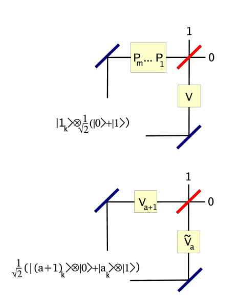
Figure 1: (Color online) Direct (upper panel) and iterative (lower panel) holonomy in the interferometer setting. In the direct scenario, the sequence $P_{1},\ldots,P_{m}$ of filtering measurements is applied to the internal state in the $0$-arm (upper path). In the $1$-arm (lower path), the internal state is exposed to a unitary operation $V$. The intensity for each orthonormal basis vector $|1_{k}\rangle$ of the initial subspace is measured in one of the output beams. Maximum of the total intensity, defined as the sum over all $k$, is obtained when $V$ coincide with the direct holonomy of the sequence. In the iterative scenario, the internal states $|a_{k}\rangle$ and $|(a+1)_{k}\rangle$ are exposed to the unitary operations $\widetilde{V}_{a}$ and $V_{a+1}$, respectively, in the two arms. Maximum of the total intensity (sum over $k$) is obtained by varying $V_{a+1}$ and keeping $\widetilde{V}_{a}$ fixed. In this way, the unitary operators $\widetilde{V}_{2},\ldots,\widetilde{V}_{m},\widetilde{V}_{1}$ are given in an iterative manner, yielding the iterative holonomy as the final unitary $\widetilde{V}_{1}$.

We first consider the direct holonomy. A beam of particles is prepared in an internal state represented by the vector $|1_{k}\rangle\in\mathcal{F}_{1}$ and divided by a 50-50 beam-splitter, yielding the state

$$|\Psi_{k}\rangle=|1_{k}\rangle\otimes\frac{1}{\sqrt{2}}\big{(}|0\rangle+|1\rangle\big{)}.$$ (12)

In the $0$-arm the internal state is exposed to the sequence $\mathcal{C}^{\prime}$ of projective filtering measurements, corresponding to the action of the projection operators $\Pi_{a}=P_{a}\otimes|0\rangle\langle 0|+\hat{1}\otimes|1\rangle\langle 1|$, $a=1,\ldots,m$. A unitary $V$ is applied to the internal degrees of freedom in the other arm. The resulting state pass a 50-50 beam-splitter. The output intensity in the $0$-arm reads

$$\mathcal{I}_{k} = \frac{1}{4}\Big{(}1+\langle 1_{k}|\Gamma^{\dagger}[\mathcal{C}]\Gamma[\mathcal{C}]|1_{k}\rangle\Big{)}$$ (13)

$$+\frac{1}{2}{\textrm{Re}}\big{[}\boldsymbol{V}^{\dagger}\boldsymbol{D}\big{]}_{kk},$$

where $\big{[}\boldsymbol{V}\big{]}_{kl}=\langle 1_{k}|V|1_{l}\rangle$ is a unitary $K\times K$ matrix and we have introduced the matrix product

$$\boldsymbol{D} = (\mathcal{F}_{1}|\mathcal{F}_{m})(\mathcal{F}_{m}|\mathcal{F}_{m-1})\ldots(\mathcal{F}_{2}|\mathcal{F}_{1}).$$ (14)

Summing over all $k$ yields the total intensity

$$\mathcal{I}_{\textrm{tot}} = \sum_{k=1}^{K}\mathcal{I}_{k}=\frac{1}{4}\Big{(}K+{\textrm{Tr}}\big{(}\Gamma^{\dagger}[\mathcal{C}]\Gamma[\mathcal{C}]\big{)}\Big{)}$$ (15)

$$+\frac{1}{2}{\textrm{Re}}{\textrm{Tr}}\big{(}\boldsymbol{V}^{\dagger}\boldsymbol{D}\big{)}.$$

Under the assumption that $\big{|}\boldsymbol{D}\big{|}^{-1}$ exists, the total intensity attains its maximum when

$$\boldsymbol{V}=\boldsymbol{U}_{D}\equiv\big{|}\boldsymbol{D}\big{|}^{-1}\boldsymbol{D}.$$ (16)

The unitary matrix $\boldsymbol{U}_{D}$ is the direct holonomy associated with the sequence $\mathcal{C}$ as measured in the interferometry setup shown in the upper panel of Fig. 1.

Next, we consider the iterative holonomy, which, as in the Abelian case, involves the performance of a sequence of interferometry experiments. Suppose all adjacent subspaces of the extended sequence $p_{1},\ldots,p_{m},p_{1}$ are overlapping. Prepare the state

$$|\Psi_{k}^{2,1}\rangle=\frac{1}{\sqrt{2}}\Big{(}V_{2}|2_{k}\rangle\otimes|0\rangle+|1_{k}\rangle\otimes|1\rangle\Big{)},$$ (17)

where $V_{2}P_{2}V_{2}^{\dagger}=P_{2}$. A 50-50 beam-splitter yields the output intensity in the $0$-arm as

$$\mathcal{I}_{k}^{2,1} = \frac{1}{4}\big{\|}|1_{k}\rangle+V_{2}|2_{k}\rangle\big{\|}^{2}$$ (18)

$$= \frac{1}{2}\Big{(}1+{\textrm{Re}}\big{[}(\mathcal{F}_{1}|\mathcal{F}_{2})\boldsymbol{V}_{2}\big{]}_{kk}\Big{)},$$

where $\big{[}\boldsymbol{V}_{2}\big{]}_{kl}=\langle 2_{k}|V_{2}|2_{l}\rangle$ is a unitary $K\times K$ matrix. Summing over $k$ yields the total intensity

$$\mathcal{I}_{\textrm{tot}}^{2,1}=\sum_{k=1}^{K}\mathcal{I}_{k}^{2,1}=\frac{1}{2}\Big{(}K+{\textrm{Re}}{\textrm{Tr}}\big{[}(\mathcal{F}_{1}|\mathcal{F}_{2})\boldsymbol{V}_{2}\big{]}\Big{)},$$ (19)

which attains its maximum for $\boldsymbol{V}_{2}=\widetilde{\boldsymbol{V}}_{2}=\boldsymbol{U}_{2,1}$. In the next step, prepare

$$|\Psi_{k}^{3,2}\rangle=\frac{1}{\sqrt{2}}\Big{(}V_{3}|3_{k}\rangle\otimes|0\rangle+\widetilde{V}_{2}|2_{k}\rangle\otimes|1\rangle\Big{)},$$ (20)

where $V_{3}P_{3}V_{3}^{\dagger}=P_{3}$ and $\langle 2_{k}|\widetilde{V}_{2}|2_{l}\rangle=\big{[}\widetilde{\boldsymbol{V}}_{2}\big{]}_{kl}$. The two beams are made to interfere by a 50-50 beam-splitter. Adding the resulting output intensities yields

$$\mathcal{I}_{\textrm{tot}}^{3,2} = \frac{1}{2}\Big{(}1+{\textrm{Re}}{\textrm{Tr}}\big{[}\boldsymbol{U}_{2,1}^{\dagger}\big{|}(\mathcal{F}_{2}|\mathcal{F}_{3})\big{|}\boldsymbol{U}_{2,1}$$ (21)

$$\times\big{(}\boldsymbol{U}_{3,2}\boldsymbol{U}_{2,1}\big{)}^{\dagger}\boldsymbol{V}_{3}\big{]}\Big{)},$$

which is maximal for $\boldsymbol{V}_{3}=\widetilde{\boldsymbol{V}}_{3}=\boldsymbol{U}_{3,2}\boldsymbol{U}_{2,1}$. By continuing in this way up to $P_{m}$ and back to $P_{1}$, we obtain the final result

$$\widetilde{\boldsymbol{V}}_{1}=\boldsymbol{U}_{I}\equiv\boldsymbol{U}_{1,m}\boldsymbol{U}_{m,m-1}\ldots\boldsymbol{U}_{2,1}.$$ (22)

The unitary matrix $\boldsymbol{U}_{I}$ is the iterative holonomy associated with $\mathcal{C}$. The interferometer setting giving rise to the iterative holonomy is illustrated in the lower panel of Fig. 1.

Under the change of frames

$$\mathcal{F}_{a}\rightarrow\Big{\{}\sum_{k=1}^{K}|a_{k}\rangle\big{[}\boldsymbol{W}_{a}\big{]}_{k,l}\Big{\}}_{l=1}^{K},\ a=1,\ldots,m,$$ (23)

$\boldsymbol{W}_{a}$ being unitary matrices, we have

$$(\mathcal{F}_{a+1}|\mathcal{F}_{a}) \rightarrow \boldsymbol{W}_{a+1}^{\dagger}(\mathcal{F}_{a+1}|\mathcal{F}_{a})\boldsymbol{W}_{a},$$

$$\boldsymbol{U}_{a+1,a} \rightarrow \boldsymbol{W}_{a+1}^{\dagger}\boldsymbol{U}_{a+1,a}\boldsymbol{W}_{a}.$$ (24)

Such a change of frames can be seen as a gauge transformation, i.e., a motion along the fiber over each of the points $p_{1},\ldots,p_{m}$ in the Grassmannian. From Eq. (24)

$$\boldsymbol{U}_{D} \rightarrow \boldsymbol{W}_{1}^{\dagger}\boldsymbol{U}_{D}\boldsymbol{W}_{1},$$

$$\boldsymbol{U}_{I} \rightarrow \boldsymbol{W}_{1}^{\dagger}\boldsymbol{U}_{I}\boldsymbol{W}_{1},$$ (25)

i.e., the direct and iterative holonomies transform unitarily (gauge covariantly) under change of frames.

The unitary matrices $\boldsymbol{U}_{D}$ and $\boldsymbol{U}_{I}$ are the non-Abelian generalizations of $\gamma_{D}$ and $\gamma_{I}$, respectively. However, while $\gamma_{D}=\gamma_{I}$, we have $\boldsymbol{U}_{D}\neq\boldsymbol{U}_{I}$ in general. There are situations, though, where the two approaches give the same result, e.g., for continuous paths in the Grassmannian. This follows from the fact that for a smooth choice of $\mathcal{F}_{s}=\{|a_{k}(s)\rangle\}_{k=1}^{K}$, we have $\big{|}(\mathcal{F}_{s+\delta s}|\mathcal{F}_{s})\big{|}=\boldsymbol{1}+O(\delta s^{2})$, $\boldsymbol{1}$ being the $K$-dimensional identity matrix. Thus, for $s\in[0,1]$ we obtain

$$\boldsymbol{D} = (\mathcal{F}_{0}|\mathcal{F}_{1})\big{(}\boldsymbol{1}+O(\delta s^{2})\big{)}\boldsymbol{U}_{1,1-\delta s}\ldots$$ (26)

$$\times\big{(}\boldsymbol{1}+O(\delta s^{2})\big{)}\boldsymbol{U}_{\delta s,0}$$

$$= (\mathcal{F}_{0}|\mathcal{F}_{1})\boldsymbol{U}_{1,1-\delta s}\ldots\boldsymbol{U}_{\delta s,0}+O(\delta s),$$

where the correction term is of order $O(\delta s)$ since it contains $\delta s^{-1}$ terms. By using the assumption that $\big{|}(\mathcal{F}_{0}|\mathcal{F}_{1})\big{|}$ is invertible and the fact that $\boldsymbol{U}_{1,1-\delta s}\ldots\boldsymbol{U}_{\delta s,0}$ is guaranteed to be unitary for sufficiently small $\delta s$, we have $\big{|}\boldsymbol{D}\big{|}=\big{|}(\mathcal{F}_{0}|\mathcal{F}_{1})\big{|}+O(\delta s)$ and $\big{|}\boldsymbol{D}\big{|}^{-1}=\big{|}(\mathcal{F}_{0}|\mathcal{F}_{1})\big{|}^{-1}+O(\delta s)$. It follows that

$$\boldsymbol{U}_{D} = \boldsymbol{U}_{0,1}\boldsymbol{U}_{1,1-\delta s}\ldots\boldsymbol{U}_{\delta s,0}+O(\delta s)$$ (27)

$$= \boldsymbol{U}_{I}+O(\delta s)$$

since $\big{|}(\mathcal{F}_{0}|\mathcal{F}_{1})\big{|}^{-1}(\mathcal{F}_{0}|\mathcal{F}_{1})=\boldsymbol{U}_{0,1}$. Thus, in the $\delta s\rightarrow 0$ limit, we obtain

$$\boldsymbol{U}_{D} = \boldsymbol{U}_{I}=\boldsymbol{U}_{0,1}{\bf P}e^{\int_{0}^{1}\boldsymbol{A}(s)ds}$$ (28)

with $[\boldsymbol{A}(s)]_{kl}=\langle\dot{a}_{k}(s)|a_{l}(s)\rangle$. In other words, in the continuous path limit, the direct and iterative holonomies are equal to the Wilczek-Zee holonomy wilczek84 for closed paths (for which $\boldsymbol{U}_{0,1}=\boldsymbol{1}$), as well as its generalization kult06 for open paths.

We finish this section by pointing out a relation between the above iterative holonomy and the Uhlmann holonomy uhlmann86 applied to a special class of density operators remark1 ; sjoqvist00 ; tong04 ; slater02 ; ericsson03 ; shi05 ; rezakhani06 . This class consists of normalized rank $K$ projectors, and we consider sequences $\frac{1}{K}P_{1},\ldots,\frac{1}{K}P_{m},\frac{1}{K}P_{1}$ of such density operators. If all the adjacent subspaces are overlapping, this is a sufficient condition for these density operators to constitute an admissible sequence uhlmann86 , for which the Uhlmann holonomy $U_{\textrm{uhl}}$ reads

$$U_{\textrm{uhl}}=\widetilde{U}_{1,m}\widetilde{U}_{m,m-1}\ldots\widetilde{U}_{2,1},$$ (29)

where $\widetilde{U}_{a+1,a}$, $a=1,\ldots,m-1$, and $\widetilde{U}_{1,m}$ are the partial isometry parts of $P_{a+1}P_{a}$ and $P_{1}P_{m}$, respectively remark2 . The overlap matrices can be written

$$(\mathcal{F}_{a+1}|\mathcal{F}_{a})_{kl} = \sum_{n}\langle(a+1)_{k}|\big{|}P_{a+1}P_{a}\big{|}|(a+1)_{n}\rangle$$ (30)

$$\times\langle(a+1)_{n}|\widetilde{U}_{a+1,a}|a_{l}\rangle,$$

where $\big{|}P_{a+1}P_{a}\big{|}$ is the positive part of $P_{a+1}P_{a}$. One can write $(\mathcal{F}_{1}|\mathcal{F}_{m})$ similarly. From Eq. (30) it follows that $[\boldsymbol{U}_{a+1,a}]_{nl}=\langle(a+1)_{n}|\widetilde{U}_{a+1,a}|a_{l}\rangle$. By combining this with Eqs. (22) and (29), and using that $\widetilde{U}_{a+1,a}=P_{a+1}\widetilde{U}_{a+1,a}$, we find

$$[\boldsymbol{U}_{I}]_{kl}=\langle 1_{k}|U_{\textrm{uhl}}|1_{l}\rangle,$$ (31)

for admissible sequences of density operators that are proportional to projectors remark3 ; aberg06 .

III Partial holonomies

If at least one pair of adjacent states in the extended sequence $\psi_{1},\ldots,\psi_{m},\psi_{1}$ are orthogonal, then the corresponding holonomies $\gamma_{D}$ and $\gamma_{I}$ are undefined. Similarly, $\boldsymbol{U}_{D}$ and $\boldsymbol{U}_{I}$ are undefined if any of the adjacent pairs of subspaces are orthogonal. However, the non-Abelian case includes partially defined holonomies, when the number of nonzero eigenvalues of the positive part of $\boldsymbol{U}_{1,m}\boldsymbol{U}_{m,m-1}\ldots\boldsymbol{U}_{2,1}\equiv\boldsymbol{I}$ or $\boldsymbol{D}$ is greater than zero but less than the subspace dimension $K$. This occurs when at least one pair of adjacent subspaces is partially overlapping, which results in a nonunique unitary part of the overlap matrix. To remove this nonuniqueness, one may use the Moore-Penrose (MP) pseudo inverse lancaster85 , denoted as $\ominus$, to introduce a well-defined concept of relative phase. Let $\mathcal{F}_{a}$ and $\mathcal{F}_{b}$ be two frames of two partially overlapping subspaces $p_{a}$ and $p_{b}$. Then the MP pseudo inverse is obtained by inverting the nonzero eigenvalues of $\big{|}(\mathcal{F}_{a}|\mathcal{F}_{b})\big{|}$ in its spectral decomposition. We define

$$\boldsymbol{U}_{a,b}=\big{|}(\mathcal{F}_{a}|\mathcal{F}_{b})\big{|}^{\ominus}(\mathcal{F}_{a}|\mathcal{F}_{b})$$ (32)

as the relative phase between the two frames. The matrix $\boldsymbol{U}_{a,b}$ is a unique partial isometry.

In Ref. kult06 , the relative phase between frames of partially overlapping subspaces was used to introduce a concept of partial holonomy of continuous open paths in the Grassmannian. Here, we develop the corresponding concepts for the discrete sequence $\mathcal{C}$.

For the direct holonomy to be (totally) defined it is a necessary and sufficient condition that all the adjacent subspaces (in the extended sequence) are overlapping remark4 . Thus, if there is partially overlapping subspaces in the sequence, and if there is at least one nonzero eigenvalue of $\big{|}\boldsymbol{D}\big{|}$, then the MP pseudo inverse yields

$$\boldsymbol{U}_{D}=\big{|}\boldsymbol{D}\big{|}^{\ominus}\boldsymbol{D},$$ (33)

which we define to be the partial direct holonomy.

In the iterative case, we again find that the holonomy becomes partial or undefined if at least one pair of adjacent subspaces in the sequence $\mathcal{C}$ is partially overlapping. For such cases, $\boldsymbol{I}$ is not unitary since at least one of the matrices $\boldsymbol{U}_{2,1},\ldots,\boldsymbol{U}_{1,m}$ is a partial isometry. If $\big{|}\boldsymbol{I}\big{|}$ has at least one nonzero eigenvalue, we define the partial isometry part of $\boldsymbol{I}$, i.e.,

$$\boldsymbol{U}_{I}=\big{|}\boldsymbol{I}\big{|}^{\ominus}\boldsymbol{I},$$ (34)

to be the partial iterative holonomy associated with $\mathcal{C}$.

Let us discuss how the partial holonomies behave under gauge transformations. From Eq. (24) we obtain

$$\boldsymbol{D} \rightarrow \boldsymbol{W}_{1}^{\dagger}\boldsymbol{D}\boldsymbol{W}_{1}\Rightarrow\big{|}\boldsymbol{D}\big{|}\rightarrow\boldsymbol{W}_{1}^{\dagger}\big{|}\boldsymbol{D}\big{|}\boldsymbol{W}_{1},$$

$$\boldsymbol{I} \rightarrow \boldsymbol{W}_{1}^{\dagger}\boldsymbol{I}\boldsymbol{W}_{1}\Rightarrow\big{|}\boldsymbol{I}\big{|}\rightarrow\boldsymbol{W}_{1}^{\dagger}\big{|}\boldsymbol{I}\big{|}\boldsymbol{W}_{1}$$ (35)

under the change of frames in Eq. (23). Furthermore, for any matrix $\boldsymbol{X}$ and unitary matrices $\boldsymbol{U}$ and $\boldsymbol{V}$ we have $(\boldsymbol{U}\boldsymbol{X}\boldsymbol{V})^{\ominus}=\boldsymbol{V}^{\dagger}\boldsymbol{X}^{\ominus}\boldsymbol{U}^{\dagger}$ (see, e.g., p. 434 in Ref. lancaster85 ). Thus,

$$\big{|}\boldsymbol{D}\big{|}^{\ominus} \rightarrow \boldsymbol{W}_{1}^{\dagger}\big{|}\boldsymbol{D}\big{|}^{\ominus}\boldsymbol{W}_{1},$$

$$\big{|}\boldsymbol{I}\big{|}^{\ominus} \rightarrow \boldsymbol{W}_{1}^{\dagger}\big{|}\boldsymbol{I}\big{|}^{\ominus}\boldsymbol{W}_{1}.$$ (36)

By combining Eqs. (35) and (36), it follows that the direct and iterative holonomies transform unitarily (gauge covariantly) also in the partial case.

We prove that the two partial holonomies in Eqs. (33) and (34) coincide with that of Ref. kult06 in the continuous path limit. To do this, we consider the smooth choice $\mathcal{F}_{s}=\{|a_{k}(s)\rangle\}_{k=1}^{K}$ and note that for sufficiently small $\delta s$, the two holonomies become partial only if $\big{|}(\mathcal{F}_{0}|\mathcal{F}_{1})\big{|}$ is not invertible. In such a case, $\big{|}\boldsymbol{D}\big{|}^{\ominus}=\big{|}(\mathcal{F}_{0}|\mathcal{F}_{1})\big{|}^{\ominus}+O(\delta s)$ and $\boldsymbol{U}_{I}=\boldsymbol{U}_{0,1}\boldsymbol{U}_{1,1-\delta s}\ldots\boldsymbol{U}_{\delta s,0}$, where $\boldsymbol{U}_{0,1}$ is a partial isometry and $\boldsymbol{U}_{1,1-\delta s}\ldots\boldsymbol{U}_{\delta s,0}$ is unitary. It follows that

$$\boldsymbol{U}_{D} = \boldsymbol{U}_{I}=\boldsymbol{U}_{0,1}{\bf P}e^{\int_{0}^{1}\boldsymbol{A}(s)ds}$$ (37)

in the $\delta s\rightarrow 0$ limit, which is the partial holonomy of Ref. kult06 .

IV Angular momentum coherent states

Consider a particle carrying an angular momentum $j$, $j\geq 1$. Let $J_{{\bf n}_{a}}$ be the angular momentum component in the direction ${\bf n}_{a}$ characterized by the spherical polar angles $\theta_{a},\phi_{a}$, i.e., ${\bf n}_{a}=(\sin\theta_{a}\cos\phi_{a},\sin\theta_{a}\sin\phi_{a},\cos\theta_{a})$. Let $\{|\mu\rangle\}_{\mu=-j}^{j}$ be the eigenbasis of $J_{z}$. Consider a sequence of filtering measurements of $J_{{\bf n}_{a}}^{2}$, $a=1,\ldots,m$, each of which selects the maximal angular momentum projection quantum numbers $\mu=\pm j$ (angular momentum coherent states peres95 ). The selection corresponds to the two-dimensional projection operators $P_{{\bf n}_{a}}=|j;{\bf n}_{a}\rangle\langle j;{\bf n}_{a}|+|-j;{\bf n}_{a}\rangle\langle-j;{\bf n}_{a}|$, $a=1,\ldots,m$, where $|\pm j;{\bf n}_{a}\rangle$ are eigenvectors of $J_{{\bf n}_{a}}$. The use of angular momentum coherent states simplifies the subsequent calculation since $|j;{\bf n}_{a}\rangle$ can be viewed as a product state of $2j$ copies of the spin-$\frac{1}{2}$ state $|\frac{1}{2};{\bf n}_{a}\rangle$, and $|-j;{\bf n}_{a}\rangle$ similarly as $2j$ copies of $|-\frac{1}{2};{\bf n}_{a}\rangle$.

Now, let ($\hbar=1$ from now on)

$$\mathcal{F}(\theta_{a},\phi_{a})=\{e^{-i\phi_{a}J_{z}}e^{-i\theta_{a}J_{y}}|\pm j\rangle\}.$$ (38)

For this choice of frames, the overlap matrix takes the form

$$(\mathcal{F}(\theta_{a},\phi_{a})|\mathcal{F}(\theta_{b},\phi_{b}))=\left(\begin{array}[]{ll}R(a,b)&S(a,b)\\ (-1)^{2j}S(a,b)^{\ast}&R(a,b)^{\ast}\end{array}\right),$$ (39)

where

$$R(a,b) = \left[\cos\left(\frac{\theta_{a}-\theta_{b}}{2}\right)\cos\left(\frac{\phi_{a}-\phi_{b}}{2}\right)\right.$$

$$\left.+i\cos\left(\frac{\theta_{a}+\theta_{b}}{2}\right)\sin\left(\frac{\phi_{a}-\phi_{b}}{2}\right)\right]^{2j},$$

$$S(a,b) = \left[\sin\left(\frac{\theta_{a}-\theta_{b}}{2}\right)\cos\left(\frac{\phi_{a}-\phi_{b}}{2}\right)\right.$$ (40)

$$\left.-i\sin\left(\frac{\theta_{a}+\theta_{b}}{2}\right)\sin\left(\frac{\phi_{a}-\phi_{b}}{2}\right)\right]^{2j}.$$

We notice that $\sqrt[j]{|R(a,b)|}+\sqrt[j]{|S(a,b)|}=1$, i.e., the overlap matrix cannot vanish for this system.

If $j$ is a half-odd integer, then

$$(\mathcal{F}(\theta_{a},\phi_{a})|\mathcal{F}(\theta_{b},\phi_{b}))$$

$$=\sqrt{|R(a,b)|^{2}+|S(a,b)|^{2}}\boldsymbol{U}_{a,b},$$ (41)

where $\boldsymbol{U}_{a,b}$ is a unique unitary matrix. It follows that the direct and iterative holonomies are identical.

When $j$ is an integer, the overlap matrix in Eq. (39) may have a nontrivial positive part. This implies that the two types of holonomies may be different. To illustrate this, consider the sequence of directions ${\bf n}_{1},{\bf n}_{2},{\bf n}_{3},{\bf n}_{4}$ characterized by the polar angles $(\theta_{0},\phi_{0})$, $(\theta_{1},\phi_{0})$, $(\theta_{1},\phi_{1})$, $(\theta_{0},\phi_{1})$, respectively. Assume that the first and third overlap matrices are degenerate. This happens for $|\theta_{1}-\theta_{0}|=\pi/2$, which yields $(\mathcal{F}(\theta_{1},\phi_{0}))|\mathcal{F}(\theta_{0},\phi_{0}))=2^{1-j}\boldsymbol{U}_{2,1}$ and $(\mathcal{F}(\theta_{0},\phi_{1}))|\mathcal{F}(\theta_{1},\phi_{1}))=2^{1-j}\boldsymbol{U}_{4,3}$. Here, $\boldsymbol{U}_{2,1}=\boldsymbol{U}_{4,3}=\frac{1}{2}\big{(}\boldsymbol{1}+\boldsymbol{\sigma}_{x}\big{)}$, where $\boldsymbol{1}$ and $\boldsymbol{\sigma}_{x}$ are the $2\times 2$ identity and Pauli$-X$ matrices, respectively. We furthermore assume that $|S(3,2)|>|R(3,2)|$ and $|S(1,4)|>|R(1,4)|$ for which a polar decomposition yields the unitary matrices $\boldsymbol{U}_{3,2}=e^{ij\chi_{1}\boldsymbol{\sigma}_{z}}$ and $\boldsymbol{U}_{1,4}=e^{-ij\chi_{0}\boldsymbol{\sigma}_{z}}$, respectively, $\boldsymbol{\sigma}_{z}$ being the Pauli-$Z$ matrix. Here, $\chi_{k}=2\arctan\big{[}\cos\theta_{k}\tan\big{(}\Delta\phi/2\big{)}\big{]}$, $k=0,1$, where $\Delta\phi=\phi_{1}-\phi_{0}$. We obtain the partial holonomies

$$\boldsymbol{U}_{D} = \frac{q_{D}}{|q_{D}|}\frac{1}{2}\left(\begin{array}[]{ll}e^{-i\eta_{0}}&e^{-i\eta_{0}}\\ e^{i\eta_{0}}&e^{i\eta_{0}}\end{array}\right),$$ (44)

$$\boldsymbol{U}_{I} = \frac{q_{I}}{|q_{I}|}\frac{1}{2}\left(\begin{array}[]{ll}e^{-ij\chi_{0}}&e^{-ij\chi_{0}}\\ e^{ij\chi_{0}}&e^{ij\chi_{0}}\end{array}\right),$$ (47)

where

$$\eta_{0} = -\arctan\left[\frac{\left(1-\sin^{2}\theta_{0}\sin^{2}\frac{\Delta\phi}{2}\right)^{j}\sin(j\chi_{0})}{\left(1-\sin^{2}\theta_{0}\sin^{2}\frac{\Delta\phi}{2}\right)^{j}\cos(j\chi_{0})+(-1)^{j}\left(\sin^{2}\theta_{0}\sin^{2}\frac{\Delta\phi}{2}\right)^{j}}\right],$$

$$q_{D} = \left(1-\sin^{2}\theta_{1}\sin^{2}\frac{\Delta\phi}{2}\right)^{j}\cos(j\chi_{1})+(-1)^{j}\left(\sin^{2}\theta_{1}\sin^{2}\frac{\Delta\phi}{2}\right)^{j},$$

$$q_{I} = \cos(j\chi_{1}).$$ (48)

It follows that the direct and iterative holonomies differ unless $q_{D}$ and $q_{I}$ have the same sign and $\eta_{0}=j\chi_{0}$. The latter happens only if $\sin^{2}\theta_{0}\sin^{2}(\Delta\phi/2)=0$. Note that $\boldsymbol{U}_{D}$ ($\boldsymbol{U}_{I}$) is undefined if $q_{D}=0$ ($q_{I}=0$).

V Conclusions

Corresponding to a sequence in the Grassmann manifold of $K$-dimensional subspaces in an $N$-dimensional Hilbert space, we have defined two holonomies, which both are gauge covariant in the sense that they transform unitarily under the change of frames in the subspaces. Interferometer settings that give rise to the two holonomies have been delineated. In the non-Abelian case these two holonomies are generically nonequivalent. In the case of one-dimensional subspaces, however, both the holonomies reduce to the standard Pancharatnam phase. Moreover, we have shown that in the limit where the sequences form a continuous and smooth path in the Grassmann manifold, the two discrete holonomies coincide with the Wilczek-Zee holonomy wilczek84 in the case of closed paths, and its generalized noncyclic version kult06 , in the open-path case. It is an interesting question whether there exist other discrete holonomies, distinct from the two considered here, that also converge to the standard holonomy in the limit of smooth curves, and if so, if those can be implemented interferometrically.

E.S. acknowledges financial support from the Swedish Research Council. J.Å. wishes to thank the Swedish Research Council for financial support and the Centre for Quantum Computation at DAMTP, Cambridge, for hospitality.

References

- (1) M. V. Berry, Proc. R. Soc. London A 392, 45 (1984).
- (2) S. Pancharatnam, Proc. Ind. Acad. Sci. A 44, 247 (1956)
- (3) F. Wilczek and A. Zee, Phys. Rev. Lett. 52, 2111 (1984).
- (4) W. Greub, S. Halperin, and R. Vanstone, Connections, Curvature and Cohomology (Academic Press, New York, 1973), Vol. II.
- (5) J. Samuel and R. Bhandari, Phys. Rev. Lett. 60, 2339 (1988).
- (6) J. Anandan and A. Pines, Phys. Lett. A 141, 335 (1989).
- (7) J. Moody, A. Shapere, and F. Wilczek, Phys. Rev. Lett. 56, 893 (1986).
- (8) R. Tycko, Phys. Rev. Lett. 58, 2281 (1987).
- (9) C. A. Mead, Phys. Rev. Lett. 59, 161 (1987).
- (10) A. Zee, Phys. Rev. A 38, 1 (1988).
- (11) J. C. Martinez, Phys. Rev. D 42, 722 (1990).
- (12) D. P. Arovas and Y. Lyanda-Geller, Phys. Rev. B 57, 12302 (1998).
- (13) R. G. Unanyan, B. W. Shore, and K. Bergmann, Phys. Rev. A 59, 2910 (1999).
- (14) P. Zanardi and M. Rasetti, Phys. Lett. A 264, 94 (1999).
- (15) J. Pachos, P. Zanardi, and M. Rasetti, Phys. Rev. A 61, 010305(R) (2000).
- (16) L. -M. Duan, J. I. Cirac, and P. Zoller, Science 292, 1695 (2001).
- (17) J. Pachos, Phys. Rev. A 66, 042318 (2002).
- (18) L. Faoro, J. Siewert, and R. Fazio, Phys. Rev. Lett. 90, 028301 (2003).
- (19) P. Solinas, P. Zanardi, and N. Zanghi, Phys. Rev. A 70, 042316 (2004).
- (20) L. -X. Cen and P. Zanardi, Phys. Rev. A 70, 052323 (2004).
- (21) I. Fuentes-Guridi, F. Girelli and E. Livine, Phys. Rev. Lett. 94, 020503 (2005).
- (22) M. S. Sarandy and D. A. Lidar, Phys. Rev. A 73, 062101 (2006).
- (23) D. Kult, J. Åberg, and E. Sjöqvist, Phys. Rev. A 74, 022106 (2006).
- (24) S. Ramaseshan and R. Nityananda, Current Science 55, 1225 (1986).
- (25) N. Mukunda and R. Simon, Ann. Phys. (N.Y.) 228, 205 (1993).
- (26) C. Nash and S. Sen, Topology and geometry for physicists (Academic Press, London, 1983).
- (27) C. A. Mead, Phys. Rev. A 44, 1473 (1991).
- (28) C. A. Mead, Rev. Mod. Phys. 64, 51 (1992).
- (29) A. Uhlmann, Rep. Math. Phys. 24, 229 (1986).
- (30) For analogous discussions concerning the relation between the Uhlmann holonomy uhlmann86 and the mixed state geometric phase sjoqvist00 ; tong04 , see Refs. slater02 ; ericsson03 ; shi05 ; rezakhani06 .
- (31) E. Sjöqvist, A. K. Pati, A. Ekert, J. S. Anandan, M. Ericsson, D. K. L. Oi, and V. Vedral, Phys. Rev. Lett. 85, 2845 (2000).
- (32) D. M. Tong, E. Sjöqvist, L. C. Kwek, and C. H. Oh, Phys. Rev. Lett. 93, 080405 (2004).
- (33) P. B. Slater, Lett. Math. Phys. 60, 123 (2002).
- (34) M. Ericsson, A. K. Pati, E. Sjöqvist, J. Brännlund, and D. K. L. Oi, Phys. Rev. Lett. 91, 090405 (2003).
- (35) M. J. Shi and J. F. Du, quant-ph/0501006.
- (36) A. T. Rezakhani and P. Zanardi, Phys. Rev. A 73, 012107 (2006).
- (37) In other words, , , and similarly for .
- (38) Although the Uhlmann holonomy for the density operators coincides with the iterative holonomy for , no such relation exists for general sequences of density operators. However, this does not rule out the possibility of an interferometric interpretation of the Uhlmann holonomy for general sequences. Indeed, such an interpretation has been provided in Ref. aberg06 .
- (39) J. Åberg, D. Kult, E. Sjöqvist, and D. K. L. Oi, quant-ph/0608185.
- (40) P. Lancaster and M. Tismenetsky, The Theory of Matrices (Academic Press, San Diego, 1985).
-
(41)
To see this, let be matrices. Then, one can show
that (see, e.g., M. Marcus and H. Minc, A survey of matrix theory
and matrix inequalities (Allyn and Bacon, Boston, 1964), p. 28)
The desired necessary and sufficient condition follows by applying this general theorem to the overlap matrices. - (42) A. Peres, Quantum theory: concepts and methods (Kluwer Academic, Dordrecht, 1995), pp. 328-329.