Quantitative entanglement witnesses

Abstract

Entanglement witnesses provide tools to detect entanglement in experimental situations without the need of having full tomographic knowledge about the state. If one estimates in an experiment an expectation value smaller than zero, one can directly infer that the state has been entangled, or specifically multi-partite entangled, in the first place. In this article, we emphasize that all these tests – based on the very same data – give rise to quantitative estimates in terms of entanglement measures: “If a test is strongly violated, one can also infer that the state was quantitatively very much entangled”. We consider various measures of entanglement, including the negativity, the entanglement of formation, and the robustness of entanglement, in the bipartite and multipartite setting. As examples, we discuss several experiments in the context of quantum state preparation that have recently been performed.

I Introduction

Entanglement witnesses have proven tremendously helpful in the experimental characterization of entanglement in composite quantum systems [1–13]. They are observables from the expectation values of which one can argue whether a prepared state is indeed entangled: whenever its expectation value takes a value smaller than zero, then one can unambiguously draw the conclusion that the state has been entangled in a particular fashion [1–4]: the entanglement has then been “witnessed”. This approach seems particularly feasible or helpful in situations where one would like to avoid to collect sufficient data to arrive at full tomographic knowledge. Specifically in multi-partite settings when detecting multi-particle entanglement this can be costly. Also in instances one can tolerate larger errors when estimating entanglement witnesses compared to the procedure where one first estimates the full state.

Originally, such a test for entanglement was thought to give rise to an answer to a “yes-no-question”: the state is entangled or it is not. Yet, in this way, one does not make use of valuable information that one has collected anyway. Actually, one has implicitly recorded data that are sufficient to make a quantitative statement: if a test is very much violated – so delivers a value much smaller than zero – then one can infer that in quantitative terms, the state was highly entangled. This quantitative statement is then meant in terms of some measure of entanglement. This is very useful information: One does not only know that the the specific entanglement property is contained in the state. But one can also give an answer to the question how useful a given state is, say, to perform a certain task of quantum information.

This article emphasizes this fact, and advocates the paradigm of quantitative tests based on data from measuring witness operators NoteThat . Needless to say, one should under all circumstances only make use of the data that have in fact been acquired in an experiment, and avoid hidden assumptions concerning the nature of the involved states. But then, in turn, one should make use of the full information that can in fact be extracted from the measurement data, including quantitative assessments.

II Paradigm of quantitative tests

The paradigm we describe is the following: imagine one has collected data from a measurement of an entanglement witness, or a collection thereof. What is the worst case scenario one could have had, concerning the degree of entanglement? Certainly, one should provide conservative estimates in this context. This is typically the practically most relevant question: one has prepared a state, and wants to know to what degree one has succeeded in doing so. This test should make use of a minimal possible number of data, or measurement settings, certainly less than full tomography. So we aim for answers to

 

“Given measurement data from measuring an entanglement witness, which one is quantitatively the least entangled state consistent with the data?”

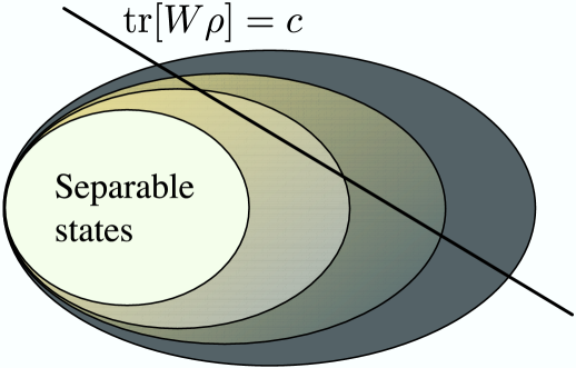
Figure 1: Schematic representation of state space. The set of separable states is depicted as the white region. The straight line represents an experimental test, so the hyperplane characterized by an entanglement witness $W$ and its expectation value $\text{tr}[\rho W]=c$. Then, one encounters a hierarchy of convex sets of states with increasing degree of entanglement, as quantified by any convex entanglement monotone.

This translates to an optimization problem: for a given measure of bi-partite or multi-partite entanglement $E$, we aim at finding the solution of

$$\min E(\rho)$$ (1)

subject to $$\rho\,\,\text{ consistent with the data},$$

or at least get reasonably good lower bounds. The general spirit of this paper will be to assume nothing more than the partial information provided by expectation values of entanglement witnesses. Based on this information, we aim at finding good bounds to entanglement measures. We also comment on the tightness of these bounds. In fact, the provided strategies often give rise to the best (tightest) possible bounds based on this partial information. The “true state” of the system is not assumed to be known, or it is not even assumed that it could in principle be measured, as full quantum tomography may be inaccessible. In turn, the optimization of entanglement witnesses, so the construction of tangent hyperplanes [11, 12, 16–19] is an interesting (and computationally provably hard) problem in its own right, which we will not touch upon here. Any known findings in this field can however immediately be applied to our setting, in that the entanglement witness that is most violated will give rise to the best bound. We hence take the entanglement witness as such and the corresponding data for granted, and will provide good bounds for entanglement measures based on them. This is actually the situation one faces when interpreting experimental data.

There is a body of work somewhat similar in spirit in the literature. The need for conservative estimates, so for minimizing the degree of entanglement in the context of a Jaynes statistical inference scheme consistent with the data was already noted in the early work Ref. Jaynes . Also, conceptually, this is related to a connection of violations of Bell inequalities to entanglement measures FM , and to quantum state estimation as in Ref. Blume .

In this work we consider the bi-partite and multi-partite setting. The system can hence be thought of consisting of a number of subsystems, such that the Hilbert space is given by ${\cal H}=\mathbbm{C}^{d_{1}}\otimes\dots\otimes\mathbbm{C}^{d_{N}}$. We assume that we have collected data that we can estimate $\{c_{1},\dots,c_{n}\}$ based on a number of entanglement witnesses $W_{1},\dots,W_{n}$, meaning that

$$\langle W_{i}\rangle=\text{tr}[W_{i}\rho]=c_{i}$$ (2)

for $i=1,\dots,n$, for example, for a single entanglement witness, $n=1$. Witness $W$ means in the bi-partite setting, $N=2$, that for all separable states

$$\rho=\sum_{i}p_{i}\rho_{i}^{(1)}\otimes\rho_{i}^{(2)}$$ (3)

on ${\cal H}=\mathbbm{C}^{d_{1}}\otimes\mathbbm{C}^{d_{2}}$ we have that [1–4]

$$\text{tr}[W\rho]\geq 0,$$ (4)

and at least for a single entangled state $\rho$, one finds that

$$\text{tr}[W\rho]<0.$$ (5)

This is very intuitive: the separable states form a convex set, and the witness defines a hyperplane in state space that separates the separable states, see Fig. 1. In the same way, one can define entanglement witnesses for the various classes of multi-particle entanglement, in a setting with Hilbert space ${\cal H}=\mathbbm{C}^{d_{1}}\otimes\dots\otimes\mathbbm{C}^{d_{N}}$. For witnesses in infinite-dimensional systems and relationships to entanglement measures, see Refs. [23–26]. In this paper, we refrain from introducing these multi-partite entanglement classes, and refer for that to Refs. [27–30].

We should mention at this point that if one allows for witnesses taking several identically prepared specimens into account, one can often improve the bounds to entanglement measures. On the positive side, this gives rise to sharper or tight bounds, often making use of few different types of measurements, or indeed even single ones [31–35]. On the negative side, one needs to implement collective operations, either with quantum networks, or in optical settings, with joint operations involving bringing together independent sources at beam splitters. Nonetheless, the first experimental measurements of a two-copy witness for arbitrary two qubit pure states was recently reported Walborn . Although we make the presented ideas explicit for the most frequently applied approach of measurements on individual specimens, it should be noted that many of the presented ideas are also applicable to this case of collective operations.

III Implications to entanglement measures

Subsequently, we will present a framework of quantitative tests, and discuss a number of bounds for different entanglement measures. We will also discuss several examples, taken from the bi-partite and multi-partite context. The concept of the conjugate function will play a central role here.

III.1 Negativity

In this first part we consider bi-partite splits of our system: so the system is either naturally bi-partite, or we group the subsystems into two parts, with joint Hilbert space ${\cal H}=\mathbbm{C}^{d_{1}}\otimes\mathbbm{C}^{d_{2}}$, with state space ${\cal S}({\cal H})$. The negativity is a measure of entanglement defined as

$$E_{N}(\rho)=\|\rho^{\Gamma}\|_{1}-1,$$ (6)

in terms of the trace-norm $\|A\|_{1}=\text{tr}|A|$. $\rho^{\Gamma}$ denotes the partial transpose of $\rho$. The negativity has been introduced in Ref.  Neg , compare also Ref. Compare , and independently shown to be an entanglement monotone in Refs. Monotone ; VidalWerner . The logarithmic version $\log_{2}\|\rho^{\Gamma}\|_{1}$ of the negativity is also an entanglement monotone Plenio , and a useful upper bound to the distillable entanglement VidalWerner ; Cost . For this measure of entanglement, we will indeed find very simple, yet tight and useful bounds.

What we are interested in here is the minimally entangled state consistent with what has been measured. So we seek the solution of

$$E_{N,\text{min}}=\inf \|\rho^{\Gamma}\|_{1}-1$$ (7)

subject to $$\text{tr}[\rho W_{i}]=c_{i},$$

$$\rho\geq 0,$$

$$\text{tr}[\rho]=1,$$

which is the desired quantity. Now, this can also be written as

$$E_{N,\text{min}}=\inf \max\text{tr}[P\rho^{\Gamma}]-1$$ (8)

subject to $$\|P\|_{\infty}=1,$$

$$\text{tr}[\rho W_{i}]=c_{i},$$

$$\rho\geq 0,$$

$$\text{tr}[\rho]=1,$$

as $\|A\|_{1}=\max\text{tr}[XA]$ with a maximation over all operators with $\|X\|_{\infty}=1$, according to the variational characterisation of the trace-norm. In turn, obviously, any such $X$ with $\|X\|_{\infty}=1$ gives rise to the lower bound

$$E_{N,\text{min}}\geq\inf \text{tr}[X\rho^{\Gamma}]-1$$ (9)

subject to $$\text{tr}[\rho W_{i}]=c_{i},$$

$$\rho\geq 0,$$

$$\text{tr}[\rho]=1.$$

We can now take an operator consisting only of the partial transposes of the witnesses we have measured,

$$X=\sum_{i=1}^{n}\alpha_{i}W_{i}^{\Gamma}+\alpha_{n+1}\mathbbm{1},$$ (10)

$\alpha_{i}\in\mathbbm{R}$ for $i=1,\dots,n+1$, such that $\|X\|_{\infty}=1$. Then, there is nothing to minimize any more, as $\text{tr}[\rho^{\Gamma}X^{\Gamma}]=\text{tr}[\rho X]$: we arrive at

$$E_{N,\text{min}}\geq\sum_{i=1}^{n}\alpha_{i}c_{i}+\alpha_{n+1}-1.$$ (11)

This is indeed a very simple bound. Yet, it is a useful, and tight one.

How can one find a suitable choice for $\alpha_{1},\dots,\alpha_{n+1}$? Any choice such that $-\mathbbm{1}\leq X\leq\mathbbm{1}$ as in Eq. (10) gives rise to a bound. In turn, one can also find the optimal choice in an efficient manner: The problem we encounter is,

$$\max \sum_{i=1}^{n}\alpha_{i}c_{i}+\alpha_{n+1}-1,$$ (12)

subject to $$-\mathbbm{1}\leq X\leq\mathbbm{1},$$

$$X=\sum_{i=1}^{n}\alpha_{i}W_{i}^{\Gamma}+\alpha_{n+1}\mathbbm{1},$$

as an optimization problem over $\{\alpha_{1},\dots,\alpha_{n+1}\}$. This is an optimization problem we can run beforehand: it is actually a semi-definite optimization problem Convex , so an optimization problem that can be efficiently solved, with certifiable error bounds. But for the use of this criterion as such, one does no longer have to solve any optimization problem.

At this point, a remark is in order concerning the tightness of the constructed bounds. Let $\rho^{\Gamma}$ be the partial transpose of a state on $\mathbbm{C}^{d_{1}}\otimes\mathbbm{C}^{d_{2}}$, $N_{p}$ eigenvalues of which are strictly positive, $N_{n}$ eigenvalues are strictly negative, and $N_{0}$ eigenvalues take the value $0$. Then any $X$ satisfying

$$\|\rho^{\Gamma}\|_{1}=\text{tr}[X\rho^{\Gamma}]$$ (13)

has a spectrum containing at least $N_{p}$ times the value $1$ and $N_{n}$ times the value $-1$. In our present context, this means that for a given system dimension $\mathbbm{C}^{d_{1}}\otimes\mathbbm{C}^{d_{2}}$, the above bound Eq. (11) is tight whenever the there exist states $\rho$ such that $S_{p}\geq N_{p}$ and $S_{n}\geq N_{n}$, where $S_{p}$ and $S_{n}$ are the number of $\pm 1$ eigenvalues of $X$, respectively. Then the bound is just saturated by actual physical states.

Example 1 (Bound to the negativity)

As a very simple example, consider states on $\mathbbm{C}^{2}\otimes\mathbbm{C}^{2}$. The witness we take is

$$W_{1}=|\phi^{-}\rangle\langle\phi^{-}|^{\Gamma},$$ (14)

which is an optimal entanglement witness, in that it is tangent to the set of separable states. Here and in the following, $|\phi^{\pm}\rangle$ and $|\psi^{\pm}\rangle$ denotes the state vectors of the familiar Bell states for two qubits. Now consider $X=-2W_{1}^{\Gamma}+\mathbbm{1}$, so $\alpha_{1}=-2$ and $\alpha_{2}=1$. The matrix $X$ clearly satisfies $\|X\|_{\infty}=1$. Then, whenever we get a value $\text{tr}[W_{1}\rho]=c$, we can assert that

$$E_{N}(\rho)\geq 2|c|.$$ (15)

It is also easy to see that this bound is tight: The spectrum of $X$ is given by $\{1,1,1,-1\}$. A family of states saturating the bound is given by

$$\rho=\lambda|\psi^{+}\rangle\langle\psi^{+}|+(1-\lambda)|\psi^{-}\rangle\langle\psi^{-}|$$ (16)

for which $E_{N}(\rho)=2|c|=|2\lambda-1|$. For $c=-1/2$, the only state consistent with this value is the maximally entangled state $|\psi^{+}\rangle\langle\psi^{+}|$, yielding $E_{N}(|\psi^{+}\rangle\langle\psi^{+}|)=1$.

In turn, we can see what we may gain from using two witnesses:

Example 2 (Bound from two witnesses)

Let us take the two entanglement witnesses $W_{i}=|\phi_{i}\rangle\langle\phi_{i}|^{\Gamma}$, $i=1,2$, where

$$|\phi_{1}\rangle = \frac{1}{10}|0,0\rangle+\frac{1}{10}|0,1\rangle+\frac{1}{5}|1,0\rangle+\left(\frac{47}{50}\right)^{1/2}|1,1\rangle,$$

$$|\phi_{2}\rangle = \frac{3}{10}|0,0\rangle+\frac{1}{10}|0,1\rangle+\frac{1}{5}|1,0\rangle+\left(\frac{7}{50}\right)^{1/2}|1,1\rangle,$$

and $c_{1}=-1/3$ and $c_{2}=-1/6$. Then, we may evaluate the optimal bound based on each witness separately, and the best bound based on both simultaneously. From solving the semi-definite optimization problem, we find in case of $W_{1}$,

$$E_{N,\text{min}}\geq 2/3,$$ (18)

then for $W_{2}$,

$$E_{N,\text{min}}\geq 1/3.$$ (19)

Indeed, in the combined case using $W_{1}$ and $W_{2}$, we obtain the better bound

$$E_{N,\text{min}}\geq 0.7375.$$ (20)

This shows that the suitable processing of several witnesses at the same time can give rise to optimized bounds. The bound arising from the data from two witnesses is stronger than each bound resulting from either of them.

The presented bounds are based on simple witnesses for qubit systems, but it should be clear that the construction is general enough such that bounds can be identified in fact for arbitrary entanglement witnesses in any dimension.

III.2 Convex hull measures and the conjugate function

Many entanglement measures are defined as a convex hull of a function, so as $\tilde{f}=cof$. This is nothing but

$$\tilde{f}(\rho)=\min\left\{\sum_{i}p_{i}f(\rho_{i}):\sum_{i}p_{i}\rho_{i}=\rho\right\},$$ (21)

for states $\rho$. The most familiar example of this sort is the entanglement of formation, for which this function $f$ is the reduced entropy function

$$f(\rho)=(S\circ\text{tr}_{2})(\rho),$$ (22)

where $\text{tr}_{2}$ is the partial trace in a bi-partite system and $S(\rho)=-\text{tr}[\rho\log_{2}\rho]$ is the von-Neumann entropy. The convex hull of a function $f$ can alternatively also be written in the form

$$\tilde{f}(\rho) = \sup_{X}\bigl{\{}\text{tr}[X\rho]:\forall|\psi\rangle\in{\cal H}:$$ (23)

$$\text{tr}[|\psi\rangle\langle\psi|X]\leq f(|\psi\rangle\langle\psi|)\bigr{\}}.$$

Note that we have for consistency assigned $f(x)=\infty$ in case of $x<0$. Again, we aim for bounding the solution of

$$E_{\text{min}}=\inf \tilde{f}(\rho),$$ (24)

subject to $$\text{tr}[\rho W_{i}]=c_{i},$$

$$\rho\geq 0,$$

$$\text{tr}[\rho]=1,$$

$i=1,\dots,n$. We can make use of the conjugate function [42–44], also known as the Legendre transform: This is defined as

$$f^{\ast}(X) = \sup_{\rho\in{\cal S}({\cal H})}\bigl{\{}\text{tr}[\rho X]-f(\rho)\bigr{\}},$$ (25)

again ${\cal S}({\cal H})$ denoting state space, which is

$$f^{\ast}(X) = \sup_{|\psi\rangle\in{\cal H}}\bigl{\{}\text{tr}[|\psi\rangle\langle\psi|X]-f(|\psi\rangle\langle\psi|)\bigr{\}}$$ (26)

for concave functions $f$. In turn, the conjugate function of the conjugate is the convex hull of the function itself Convex : In other words, since the entanglement of formation is the convex hull of the reduced entropy function itself, we have that

$$f^{\ast\ast}(\rho)=\tilde{f}(\rho),$$ (27)

where

$$f^{\ast\ast}(\rho)=\sup_{X}\bigl{\{}\text{tr}[\rho X]-f^{\ast}(X)\bigr{\}}.$$ (28)

By definition, $f^{\ast}(X+\alpha\mathbbm{1})=f^{\ast}(X)+\alpha$ for any $X$. Now, for any

$$X=\sum_{i=1}^{n}\alpha_{i}W_{i},$$ (29)

we indeed arrive at the bound

$$E_{\text{min}}\geq\sum_{i=1}^{n}c_{i}\alpha_{i}-f^{\ast}(X),$$ (30)

in terms of the conjugate function $f^{\ast}$ of $f$. In this way, we do not have to evaluate the convex hull explicitly.

Moreover, the bounds constructed in this way are always tight. It follows from the duality of the convex hull of the function and its Legendre transform that the bounds are tight when varying over all $\{\alpha_{1},\dots,\alpha_{n}\}$. There always exists a state $\rho$ satisfying $E_{\text{min}}=f^{\ast\ast}(\rho)$, so for example $E_{F,\text{min}}=E_{F}(\rho)$ for the entanglement of formation. In this sense, the given bounds are the best possible bounds of this form.

In case a symmetry can be identified, the estimation of the conjugate function of a given function can be simplified. To bring the conjugate function into a form that is more accessible to numerical assessments, we can proceed as follows: If $f=(g\circ{\text{tr}}_{2})$, and $g$ is concave, we can define

$$g(\rho) = \inf_{Y}\{\text{tr}[Y\rho]-g^{\prime}(Y)\},$$ (31)

$$g^{\prime}(Y) = \inf_{\rho}\{\text{tr}[Y\rho]-g(\rho)\},$$ (32)

and can write the above conjugate function as (assuming that $X$ and $Y_{1}$ are Hermitian)

$$f^{\ast}(X) = \sup_{\rho}\sup_{Y_{1}}\left\{\text{tr}[(X-(Y_{1}\otimes\mathbbm{1}))\rho]+g^{\prime}(Y_{1})\right\}$$ (33)

$$= \sup_{Y_{1}}\left\{\lambda_{\max}(X-(Y_{1}\otimes\mathbbm{1}))+g^{\prime}(Y_{1})\right\}.$$

For the entropy function $g(x)=-x\log_{2}x$, for example, the conjugate $g^{\prime}$ is known, and one finds Convex

$$g^{\prime}(Y_{1})=-\log_{2}\text{tr}[\exp({-Y_{1}\log 2})].$$ (34)

In this form, the problem is in a suitable form for such numerical assessments. The resulting bound is then a combination of the numerically evaluated expression and the value for $c$ from the actual data. In practice, this numerical evaluation amounts to a global optimization problem, which can, for a small number of parameters in typical problems in the quantum information context, be solved for an arbitrary witness. Also, semi-definite relaxations as in Refs. Hierarchy ; Lasserre readily give rise to certifiable bounds.

As an example, let us look at the entanglement of formation, and a single witness $W_{1}$. Then,

$$E_{F,\text{min}} \geq \alpha_{1}c-f^{\ast}(\alpha_{1}W_{1}),$$ (35)

with $\alpha_{1}\in\mathbbm{R}$, so any choice for $\alpha_{1}$ delivers a bound. Obviously, an optimal bound is achieved using

$$E_{F,\text{min}}\geq\text{sup}_{\alpha_{1}}\left\{\alpha_{1}c-f^{\ast}(\alpha_{1}W_{1})\right\}.$$ (36)

Similarly, more than a single witness can be considered. So one needs to find good upper bounds to $f^{\ast}(\alpha_{1}W_{1})$.

Example 3 (Bound to the entanglement of formation)

This becomes particularly simple for witnesses of the form $W_{1}=|\phi\rangle\langle\phi|^{\Gamma}$ in $\mathbbm{C}^{d}\otimes\mathbbm{C}^{d}$, for entangled state vectors $|\phi\rangle$. We consider the conjugate function $f^{*}$, evaluated at $\alpha_{1}W_{1}$. It is easily seen from Eq. (23) that, for any entanglement measure, the conjugate function is invariant under local unitaries. Then, without loss of generality $|\phi\rangle$ can be taken to be of Schmidt form

$$|\phi\rangle=\sum_{i=1}^{d}\xi_{i}|i,i\rangle.$$ (37)

The partial transpose $|\phi\rangle\langle\phi|^{\Gamma}$ gives rise to the form

$$|\phi\rangle\langle\phi|^{\Gamma}=\sum_{j,k=1}^{d}\xi_{j}\xi_{k}|j,k\rangle\langle k,j|,$$ (38)

so in a product basis a direct sum of $1\times 1$ and $2\times 2$ matrices. We seek the maximal value of $\alpha_{1}\text{tr}[W_{1}|\psi\rangle\langle\psi|]$ and a minimal value for $f(|\psi\rangle\langle\psi|)$. Let

$$w=\max_{i,j\in\{1,\dots,d\},\,i<j}\{\xi_{i}\xi_{j}\},$$ (39)

so $w=\xi_{k}\xi_{l}$ for some $k,l=1,\dots,d$. It is not difficult to see that then the optimal state vector $|\psi\rangle$ takes the form

$$|\psi\rangle=a|k,l\rangle-(1-a^{2})^{1/2}|l,k\rangle$$ (40)

for some $a\in[0,1]$. This state vector gives rise to

$$\text{tr}[-W_{1}|\psi\rangle\langle\psi|]=2a(1-a^{2})^{1/2}w$$ (41)

and $f(|\psi\rangle\langle\psi|)=-a^{2}\log_{2}a^{2}-(1-a^{2})\log_{2}(1-a^{2})$, defining the concave (classical entropy) function $h(x)=-x\log_{2}x-(1-x)\log_{2}(1-x)$ and the concave function $g(x)=({x(1-x)})^{1/2}$,

$$f^{\ast}(\alpha_{1}W_{1}) = \sup_{a\in[0,1]}\biggl{\{}-2\alpha_{1}wa(1-a^{2})^{1/2}$$ (42)

$$+ a^{2}\log_{2}a^{2}+(1-a^{2})\log_{2}(1-a^{2})\biggr{\}}$$

$$= \sup_{p\in[0,1]}\bigl{\{}-2\alpha_{1}wg(p)-h(p)\bigr{\}}.$$

We can distinguish three regimes. Define the parameter $b=-2\alpha_{1}w$ and the function $z(p)=bg(p)-h(p)$. The second derivative of $z$ is given by

$$z^{\prime\prime}(p)=\frac{1}{\log(2)p(1-p)}-\frac{b}{4(p(1-p))^{3/2}}.$$ (43)

The function $z$ is convex iff $z^{\prime\prime}$ is non-negative for all $p\in[0,1]$, which occurs when

$$b\leq\min_{p}\frac{4({p(1-p)})^{1/2}}{\log(2)}=0.$$ (44)

The function is concave when $z^{\prime\prime}$ is non-positive for all $p$, which occurs when

$$b\geq\max_{p}{4{p(1-p)}^{1/2}}/{\log(2)}=2/\log(2)=2.88539.$$ (45)

In between these values, $z$ is neither convex nor concave. If $z$ is convex ($b\leq 0$), its supremum occurs at one of the extreme points, either $p=0$ or $p=1$. But of course, either one gives the same value, namely $0$. If $z$ is concave ($b\geq 2/\log(2)$), it has one supremum. By the even symmetry of $z$ around $p=1/2$, the supremum must occur at $p=1/2$, yielding as supremum value $(b-2)/2$. For determining the supremum in the case $0\leq b\leq 2/\log(2)$, a transcendental equation has to be solved. The supremum as function of $b$ can be approximated from above by the polynomial

$$0.001876b + 0.008239b^{2}+0.019733b^{3}$$

$$- 0.005649b^{4}+0.001430b^{5}.$$

The average error of this approximation is $0.00017$. We may take $\alpha_{1}=-1/w$, then $f^{\ast}(\alpha_{1}W_{1})\leq c_{0}$ with $c_{0}=0.14985$. Therefore, we obtain the bound

$$E_{F,\text{min}}\geq|c|/|w|-c_{0}.$$ (47)

To emphasize that again, we do not assume the “true state” to be detected to be known or accessible. For completeness, we do elaborate on an example showing the tightness of the bound. For example, for the family of states in Eq. (16) for $\lambda\in[1/2,1]$, and for the witness $W_{1}=|\phi^{-}\rangle\langle\phi^{-}|^{\Gamma}$ as in Eq. (14), we find $2|c|=|2\lambda-1|$, $w=1/2$, and in fact

$$E_{F}(\rho)=h\left(1/2+(\lambda(1-\lambda))^{1/2}\right),$$ (48)

which has to be compared with

$$E_{F,\text{min}}\geq|2\lambda-1|-c_{0}.$$ (49)

As can easily be seen, this is a very good lower bound (as a tangent the best possible affine bound), and the bound is tight for $\lambda=0.7056$.

Example 4 (Second bound to the entanglement of formation)

Let us consider a witness of the common form

$$W_{1}=a\mathbbm{1}-b|\phi\rangle\langle\phi|$$ (50)

with $a,b>0$. The conjugate function can be easily written as

$$f^{\ast}(\alpha_{1}W_{1})=\sup_{|\psi\rangle\in{\cal H}}\bigl{\{}\alpha_{1}a-\alpha_{1}b|\langle\phi|\psi\rangle|^{2}-f(|\psi\rangle\langle\psi|)\bigr{\}}.$$ (51)

We assume $|\phi\rangle$ to be in its Schmidt form, given by Eq. (37). The state vector $|\psi\rangle$ might also be written as

$$|\psi\rangle=\sum_{i=1}^{d}\mu_{i}|i^{\prime},i^{\prime}\rangle,$$ (52)

where the basis $\{|i^{\prime}\rangle\}$ is not necessarily equal to the Schmidt basis $\{|i\rangle\}$ of $|\phi\rangle$. One can thus minimize over the basis $\{|i^{\prime}\rangle\}$ and the Schmidt coefficients $\mu_{i}$. The last term in the right hand side of Eq. (51) clearly does not depend on $\{|i^{\prime}\rangle\}$. In turn, given a fixed set of Schmidt coefficients $\mu_{i}$, this implies that the optimal basis will be the one which maximizes the overlap $|\langle\phi|\psi\rangle|^{2}$. It can be easily shown that the maximum is obtained when choosing $\{|i^{\prime}\rangle\}$ to be equal to the Schmidt basis of $|\phi\rangle$. Therefore, we are left with an easier maximization problem, over the Schmidt coefficients only, given by

$$f^{\ast}(\alpha_{1}W_{1}) = \sup_{\{\mu_{i}\}}\biggl{\{}\alpha_{1}a-\alpha_{1}b\biggl{(}\sum_{i}\xi_{i}\mu_{i}\biggr{)}^{2}$$

$$+ \sum_{i}\mu_{i}^{2}\log_{2}(\mu_{i}^{2})\biggr{\}}.$$

Although it is not possible to solve Eq. (4) analytically in terms of $\alpha_{1},a$ and $b$ for all choices, it can be easily numerically evaluated. For example, let us consider $a=\alpha_{1}=1$, $b=3/2$, and

$$|\phi\rangle=\left({\frac{1}{3}}\right)^{1/2}|0,0\rangle+\left({\frac{2}{3}}\right)^{1/2}|1,1\rangle,$$ (54)

so $\xi_{1}=(1/3)^{1/2}$ and $\xi_{2}=(2/3)^{1/2}$. We then get the following bound for the entanglement of formation

$$E_{F,\text{min}}\geq|c|-0.5550.$$ (55)

Example 5 (Bounds from Renyi entropies)

Since for the entropy function $f$, we have that

$$f(x)\geq g_{q}(x)=\frac{1}{1-q}\log_{2}(x^{q})$$ (56)

for $q>1$, we get an upper bound to $f^{\ast}(X)$ as

$$f^{\ast}(X)\leq\sup_{|\psi\rangle}\bigl{\{}\text{tr}[|\psi\rangle\langle\psi|X]-g_{q}(|\psi\rangle\langle\psi|)\bigr{\}}.$$ (57)

The function $g_{q}$ is no longer concave, but we nevertheless get an appropriate bound when optimizing over pure states. Particularly useful is the case of $q=2$, when we merely need to evaluate $\text{tr}[\text{tr}_{2}[|\psi\rangle\langle\psi|]^{2}]$.

Further bounds can, e.g., be found in Refs. Breuer ; Chen .

III.3 Remarks on exploiting symmetry

If one has a witness which is invariant under a local symmetry group, one can in instances simplify the evaluation of good bounds under the constraint provided by the entanglement witness: One can take the Haar average with respect to that group, which will always diminish the degree of entanglement. So a twirling with respect to a, for example, $U\otimes U$, $U\otimes U^{\ast}$, or $O\otimes O$-symmetry, or one corresponding to $SU(2)$ or symmetric group representations, can only give a lower bound Vollbrecht : For any convex entanglement monotone $f$,

$$E_{\text{min}}=\inf f(\rho)$$ (58)

subject to $$\text{tr}[\rho W_{1}]=c_{1},$$

$$\rho\text{ is a symmetric state}.$$

Hence, we have to evaluate an entanglement measure under symmetry [49–53], given the constraint.

Example 6 (Symmetry)

To give a very simple example, let us consider a witness of the form

$$W_{1}=a\mathbbm{1}+b|\phi^{-}\rangle\langle\phi^{-}|^{\Gamma}$$ (59)

for some $a,b\in\mathbbm{R}$ and for states on $\mathbbm{C}^{2}\otimes\mathbbm{C}^{2}$. Since $|\phi^{-}\rangle\langle\phi^{-}|$ is a $U\otimes U$-symmetric state, this witness is $U\otimes U^{\ast}$-symmetric. Therefore, we can optimize the bound with respect to $U\otimes U^{\ast}$-symmetric states, which is the one-dimensional convex set

$$\rho=\lambda\mathbbm{1}/4+(1-\lambda)|\psi^{+}\rangle\langle\psi^{+}|,$$ (60)

for $\lambda\in[0,1]$. The entanglement of formation $E_{F}(\rho)$ of such symmetric states $\rho$, in turn, is known Vollbrecht .

III.4 Concurrence

An interesting example where the conjugate function can be analytically calculated is the concurrence of two qubits Wootters . Let us define the following basis for $\mathbbm{C}^{2}\otimes\mathbbm{C}^{2}$,

$$|\Psi_{0}\rangle=\frac{1}{\sqrt{2}}(|0,0\rangle+|1,1\rangle),|\Psi_{1}\rangle=\frac{i}{\sqrt{2}}(|0,0\rangle-|1,1\rangle),$$ (61)

$$|\Psi_{2}\rangle=\frac{i}{\sqrt{2}}(|0,1\rangle+|1,0\rangle),|\Psi_{3}\rangle=\frac{1}{\sqrt{2}}(|0,1\rangle-|1,0\rangle).$$ (62)

As is well-known, a general two-qubit pure state can then be written as

$$|\phi(c)\rangle=\sum_{i=0}^{3}c_{i}|\Psi_{i}\rangle.$$ (63)

The concurrence of a pure state is defined as

$$C(|\psi\rangle\langle\psi|)=\left|\sum_{i=0}^{3}c_{i}^{2}\right|,$$ (64)

and extended to mixed states by a convex hull construction. The importance of the concurrence is twofold. On one hand, it is intimately related to the entanglement of formation of two qubits. Indeed, given the concurrence of a two qubit state $\rho$, its entanglement of formation reads Wootters

$$E_{F}(\rho)=H\left(\frac{1}{2}\left(1+(1-C(\rho)^{2})^{1/2}\right)\right).$$ (65)

On the other hand, an analytical expression for the concurrence of a general two qubits mixed state is known Wootters , which in turn implies an analytical formula for the entanglement of formation.

The first interesting bound to the concurrence based on a witness, derived in Ref. VerstraetePhD , is given by

$$C(\rho)=\max\left\{0,-\min_{A\in SL(2,\mathbbm{C})}\text{tr}[|A\rangle\langle A|^{\Gamma}\rho]\right\},$$ (66)

where $|A\rangle$ denotes the unnormalized state vector $(A\otimes\mathbbm{1})|I\rangle$ with $|I\rangle=|0,0\rangle+|1,1\rangle$ and $A$ is any (in its determinant normalized) $2\times 2$ invertible matrix. It is thus seen that any witness $W_{1}$ of the form

$$W_{1}=|A\rangle\langle A|^{\Gamma}$$ (67)

provides a lower bound to the concurrence. Note that this class of witnesses is exactly the class of optimal entanglement witnesses of two qubits, where optimality refers to the robustness with respect to white noise (mixing with the identity).

Although Eq. (66) constitutes a useful tool to estimate $C$, it has the drawback that only witnesses of the restricted form given by Eq. (67) can be used. On the other hand, the method based on conjugate functions, oulined in the previous subsection, can be applied to any entanglement witness. We now aim at showing that the conjugate function of the concurrence can be evaluated analytically.

The concurrence can be expressed as the convex-hull of the function

$$f(\rho)=\left(2(1-\text{tr}[\text{tr}_{2}[\rho]^{2}])\right)^{1/2},$$ (68)

defined on states $\rho$. It is easy to check that $f$ is concave. This in turn implies that the supremum in Eq. (26) can be calculated over pure states only. The conjugate function $f^{*}$ can be expressed as the following optimization problem,

$$f^{*}(X) = \sup_{\{c_{i}\}}\sum_{i,j}\langle\Psi_{i}|X|\Psi_{j}\rangle c_{i}^{*}c_{j}-|\sum_{c_{i}}c_{i}^{2}|,$$ (69)

subject to $$|\phi\rangle=\sum_{i}c_{i}|\Psi_{i}\rangle\text{ is normalized.}$$

The optimal solution, as a function of $X$, although this not being a convex problem, can be readily evaluated with the help of a computer algebra program Alg .

III.5 Further convex roof measures

Note that we considered the entanglement of formation as an example for a “convex roof measure”. There are other important measures of entanglement in the multi-partite context, where the presented ideas can be applied. This applies in particular to the geometric measure of entanglement. This is a measure for entanglement in the multi-partite case, which is defined for pure states as Geometric

$$E_{G}(|\psi\rangle\langle\psi|)=\inf_{\rho}\||\psi\rangle\langle\psi|-\rho\|_{2},$$ (70)

where $\|A\|_{2}=\text{tr}[A^{2}]$ is the Hilbert-Schmidt norm, and the infimum is taken with respect to all pure product states. The extension to mixed states is done via a convex roof construction. Similarly, the global entanglement of Ref. Global may be considered. Both quantities are proper multi-partite entanglement monotones. For a survey on multi-partite entanglement measures, see, e.g., Refs. Multi3 ; PlenioMeasures .

III.6 Robustness

Given a bi-partite or multi-partite state $\rho$, its generalized robustness of entanglement – introduced in Refs. VidalTarrach ; Steiner – is defined as the minimal $s>0$ such that the state

$$\omega=\frac{\rho+s\sigma}{1+s}$$ (71)

is separable, where $\sigma$ is another arbitrary state. This measure can be interpreted as the minimum amount of noise necessary to wash out completely the quantum correlations initially present in the state $\rho$. In addition, the generalized robustness also has the operational interpretation for bi-partite systems as the usefulness of the state in question as an ancilla in teleportation protocols Brandao2 and is a multi-partite entanglement monotone Brandao1 .

For our purposes, a very convenient representation of the generalized robustness, obtained as the Lagrange dual form Convex of Eq. (71) Brandao1 , is

$$E_{R}(\rho)=\max\left\{0,-\min_{W}\text{tr}[W\rho]\right\},$$ (72)

where $W$ is varied over the set of witnesses with maximum eigenvalue smaller than unity ($W\leq\mathbbm{1}$). Note that by considering different sets of witnesses, one can quantify all the different kinds of multi-partite entanglement [27–29].

As discussed in Refs. Brandao1 ; Cavalcanti , it follows directly from Eq. (73) that the expectation value of any measured witness $W$ gives rise to a useful lower bound to the generalized robustness. Then, when $\text{tr}[W\rho]=c<0$,

$$E_{R,\text{min}}(\rho)\geq|c|/{\lambda_{\max}(W)}.$$ (73)

In full generality, this same approach can be applied to any entanglement measure which can be expressed as

$$E(\rho)=\max\left\{0,-\min_{W\in{\cal M}}\text{tr}[W\rho]\right\},$$ (74)

where ${\cal M}$ is the intersection of the sets of entanglement witnesses with some other set (e.g., the set $W\leq\mathbbm{1}$). Interestingly, several other well-known entanglement quantifiers, such as the best separable approximation Karnas , the Rains fidelity of teleportation Rains , and the concurrence (see Eq. (64)), fit into this classification. Here for concreteness we focus on the generalized robustness and on the random robustness, which we discuss in the sequel.

A source of noise often considered in experiments is so-called white noise, in which the initial state $\rho$ is driven to a state of the form

$$\rho\mapsto\rho+s\frac{\mathbbm{1}}{D},$$ (75)

where $s$ is related to the amount of noise introduced in the system. Here $D$ stands for the dimension of the Hilbert space which $\rho$ acts on. In this sense, it is interesting to ask what is the maximal tolerance of an entangled state to white noise, before all its initially entanglement is transformed into merely classical correlations. The random robustness VidalTarrach is exactly such a quantity. In the framework of Eq. (74), we can express it as the minimization over the set of entanglement witnesses with trace equal to $D$. Hence, every entanglement witness $W$ can be used to lower bound it as

$$E_{r,\text{min}}(\rho)\geq\frac{D|c|}{\text{tr}[W]},$$ (76)

again with $\text{tr}[W\rho]=c$.

Example 7 (Tri- and quadripartite photonic entanglement)

As an example, we consider two multi-partite witnesses which have been measured in the photonic parametric-down-conversion experiment of Ref. WeinDetect , so $N=3$ and $N=4$. Consider the following multi-partite pure states vectors

$$|W\rangle=\frac{1}{\sqrt{3}}(|0,0,1\rangle+|0,1,0\rangle+|1,0,0\rangle)$$ (77)

and

$$|\Psi^{(4)}\rangle=\frac{1}{\sqrt{3}}(|0,0,1,1\rangle+|1,1,0,0\rangle$$

$$- \frac{1}{2}(|0,1,1,0\rangle+|1,0,0,1\rangle+|0,1,0,1\rangle+|1,0,1,0\rangle)).$$

Then the two associated multi-partite entanglement witnesses which have been measured are given by

$$W_{W} = \frac{2}{3}\mathbbm{1}-|W\rangle\langle W|,$$ (79)

$$W_{\Psi^{(4)}} = \frac{3}{4}\mathbbm{1}-|\Psi^{(4)}\rangle\langle\Psi^{(4)}|.$$ (80)

Whereas the witness $W_{W}$ detects genuine tri-partite entanglement, having positive values on separable and bi-partite entangled states, the operator $W_{\Psi^{(4)}}$ witnesses genuine four-partite entanglement, being positive on separable, bi-separable, and tri-separable states. The measured expectation values in turn are WeinDetect ,

$$\text{tr}[W_{W}\rho] = -0.197\pm 0.018,$$ (81)

$$\text{tr}[W_{\Psi^{(4)}}\rho] = -0.151\pm 0.010.$$ (82)

Hence we readily have the following estimates on the robustness of the, a priori unknown, measured states $\rho_{1}$ and $\rho_{2}$, consiting of three and four parties respectively:

$$E_{R,\text{min}}(\rho_{1}) \geq 0.2955\pm 0.027,\hskip 5.69046ptE_{r,\text{min}}(\rho_{1})\geq 0.360\pm 0.096,$$

$$E_{R,\text{min}}(\rho_{2}) \geq 0.201\pm 0.013,\hskip 5.69046ptE_{r,\text{min}}(\rho_{2})\geq 0.220\pm 0.021.$$

Example 8 (Four-photon graph state)

In Ref. NewWein , entanglement witnesses have been employed to characterize optical four-photon graph states[70–74] that have been prepared from entangled photon pairs, followed by a controlled-phase gate (compare also Ref. ZeilingerCluster ). For the four-photon cluster state BriegelPersistentEntanglement , $N=4$, the given witness is

$$W_{{\cal C}^{(4)}} = 3\mathbbm{1}-\frac{1}{2}\left(Z^{(1)}Z^{(2)}+\mathbbm{1}\right)\left(Z^{(2)}X^{(3)}X^{(4)}+\mathbbm{1}\right)$$ (84)

$$- \frac{1}{2}\left(X^{(1)}X^{(2)}Z^{(3)}+\mathbbm{1}\right)\left(Z^{(3)}Z^{(4)}+\mathbbm{1}\right).$$

The maximal theoretical value is $\text{tr}[W_{{\cal C}^{(4)}}\rho]=-1$, the measured value is

$$\text{tr}[W_{{\cal C}^{(4)}}\rho]=-0.299\pm 0.050.$$ (85)

This gives rise to

$$E_{R,\text{min}} \geq 0.0997\pm 0.0167,$$ (86)

$$E_{r,\text{min}} \geq 0.1120\pm 0.020.$$ (87)

Example 9 (Quantum byte)

In the recent spectacular experiment of Ref.  Byte , $8$ ions have been prepared in a multi-particle entangled state. The multi-particle entanglement has in turn been demonstrated using the concept of entanglement witnesses. In order to introduce the multi-partite entanglement witnesses that have been measured, we have to consider the $N$-partite $W$ states

$$|W_{N}\rangle = (|0,\dots,0,0,1\rangle+|0,\dots,0,1,0\rangle$$

$$+ |0,\dots,1,0,0\rangle+\dots+|1,\dots,0,0,0\rangle)/\sqrt{N}.$$

Define the $N$-qubit state vectors $|BS_{i}\rangle=|D_{i}\rangle\otimes|W_{N-1}\rangle$, which consist of $|0\rangle$ on the $i$-th qubit and the state vector $|W_{N-1}\rangle$ on the remaining qubits, and the corresponding operators

$${\cal Q}_{N}=10|W_{N}\rangle\langle W_{N}|-\beta_{N}\sum_{i=1}^{N}|BS_{i}\rangle\langle BS_{i}|,$$ (89)

where $\beta_{N}$ is a fixed real number for each value. Next, define $\gamma_{N}=\max_{|\Psi\rangle=|a\rangle\otimes|b\rangle}\langle\Psi|{\cal Q}|\Psi\rangle$, where $|\Psi\rangle$ ranges over all possible bi-separable state vectors Multi1 ; Multi3 with respect to all possible bi-partitions. The witnesses are then given by

$$W_{\text{Byte}}=\gamma_{N}\mathbbm{1}-{\cal Q}_{N}.$$ (90)

They hence classify tri-partite entanglement. As explained in Ref. Byte , the expectation values reported refer to the normalized versions of ${W}_{\text{Byte}}$ with $\text{tr}[{W}_{\text{Byte}}]=2^{N}$, where $N$ is the number of parties of the state. Therefore, we can readily read them as lower bounds to the random robustness of the unknown $3$, $4$, $5$, $6$, $7$, and $8$ qubit states:

$$E_{r,\text{min}}(3) \geq 0.532,\hskip 5.69046ptE_{r,\text{min}}(4)\geq 0.460,\hskip 5.69046pt$$ (91)

$$E_{r,\text{min}}(5) \geq 0.202,\hskip 5.69046ptE_{r,\text{min}}(6)\geq 0.271,\hskip 5.69046pt$$ (92)

$$E_{r,\text{min}}(7) \geq 0.071,\hskip 5.69046ptE_{r,\text{min}}(8)\geq 0.029.\hskip 5.69046pt$$ (93)

Needless to say, the same discussion can also be performed based on other multi-partite measures of entanglement, such as the geometric measure of entanglement.

IV Conclusions

In this work, we have introduced quantitative bounds to entanglement measures, on the basis of expectation values of entanglement witnesses. In this way, quantities that are frequently measured in order to detect entanglement in experimental settings can be augmented with a stronger, quantitative statement on the degree of entanglement. In most instances, this does not require any additional effort at all, but these quantitative bounds may even be added in retrodiction. Several measures of entanglement have been considered. Needless to say, similar methods can also be made use of if one has additional knowledge at hand about the system, say, from correlation measurements.

We have considered the concept of the conjugate function in this context, and have presented a number of new bounds to entanglement measures. For the negativity, simple and very useful bounds emerged from a variational principle. We have discussed several examples taken from experimental settings, both from the context of linear optics, as well as of trapped ions. In this way, we have sharpened the notion that if a test for entanglement is indeed violated to a large extent, then the degree of entanglement can be expected to be large.

V Acknowledgements

We would like to thank O. Gühne, M. Reimpell, and R.F. Werner for valuable discussions on the subject of the paper and P. Hyllus for very helpful comments on the manuscript. This work has been coordinated in submission with their independent work Ref. BS . Note also that the independent work Ref. Martin (which was made available slightly later on the preprint server) is similar in its spirit, and strongly and nicely complements the present work in that the role of correlation measurements is emphasized and studied in great detail. The semi-definite program was programmed using the packages SeDuMi and Yalmip. This work has been supported by the DFG (SPP 1116, SPP 1078), the EU (QAP), the EPSRC, the QIP-IRC, Microsoft Research, the Brazilian agency Conselho Nacional de Desenvolvimento Científico e Tecnológico (CNPq), and the EURYI Award Scheme.

References

- (1) M. Horodecki, P. Horodecki, and R. Horodecki, Phys. Lett. A 223, 1 (1996).
- (2) B.M. Terhal, Phys. Lett. A 271, 319 (2000).
- (3) B.M. Terhal, J. Th. Comp. Sc. 287, 313 (2002).
- (4) D. Bruss, J.I. Cirac, P. Horodecki, F. Hulpke, B. Kraus, M. Lewenstein, and A. Sanpera, J. Mod. Opt. 49, 1399 (2002).
- (5) M. Bourennane, M. Eibl, C. Kurtsiefer S. Gaertner, H. Weinfurter, O. Gühne, P. Hyllus, D. Bruss, M. Lewenstein, and A. Sanpera, Phys. Rev. Lett. 92, 087902 (2004).
- (6) N. Kiesel, C. Schmid, U. Weber, O. Gühne, G. Toth, R. Ursin, and H. Weinfurter, Phys. Rev. Lett. 95, 210502 (2005).
- (7) H. Häffner, W. Hänsel, C.F. Roos, J. Benhelm, D. Chek-al-kar, M. Chwalla, T. Körber, U.D. Rapol, M. Riebe, P.O. Schmidt, C. Becher, O. Gühne, W. Dür, and R. Blatt, Nature 438, 643 (2005).
- (8) C. Becher, J. Benhelm, D. Chek-Al-Kar, M. Chwalla, H. Häffner, W. Hänsel, T. Körber, A. Kreuter, G.P.T. Lancaster, T. Monz, E.S. Phillips, U.D. Rapol, M. Riebe, C.F. Roos, C. Russo, F. Schmidt-Kaler, and R. Blatt, Entanglement of trapped ions, Proc. 17th Int. Conf. Laser Spectroscopy, Cairngorms National Park, Scotland, 2005, Eds. E.A. Hinds, A. Ferguson, and E. Ries, World Scientific.
- (9) G. Toth and O. Gühne, Phys. Rev. Lett. 94, 060501 (2005).
- (10) O. Gühne, P. Hyllus, D. Bruss, A. Ekert, M. Lewenstein, C. Macchiavello, and A. Sanpera, J. Mod. Phys. 50, 1079 (2003).
- (11) J. Eisert, P. Hyllus, O. Gühne, and M. Curty, Phys. Rev. A 70, 062317 (2004).
- (12) A.C. Doherty, P.A. Parrilo, and F.M. Spedalieri, Phys. Rev. A 71, 032333 (2005).
- (13) G.A. Durkin and C. Simon, Phys. Rev. Lett. 95 180402 (2005).
- (14) Note that in the independent work Ref. BS , O. Gühne, M. Reimpell, and R.F. Werner came to similar conclusions, and the two submissions have been coordinated.
- (15) O. Gühne, M. Reimpell, and R.F. Werner, quant-ph/0607163.
- (16) M. Lewenstein, B. Kraus, J.I. Cirac, and P. Horodecki, Phys. Rev. A 62, 052310 (2000).
- (17) L. Gurvits, Proceedings of the thirty-fifth ACM symposium on theory of computing, San Diego, CA, USA (2003).
- (18) F.G.S.L. Brandão and R.O. Vianna, Phys. Rev. Lett. 93, 220503 (2004).
- (19) L.M. Ioannou and B.C. Travaglione, Phys. Rev. A 73, 052314 (2006).
- (20) R. Horodecki, M. Horodecki, and P. Horodecki, Phys. Rev. A 59, 1799 (1999).
- (21) F. Verstraete and M.M. Wolf, Phys. Rev. Lett. 89, 170401 (2002).
- (22) R. Blume-Kohout and P. Hayden, quant-ph/0603116.
- (23) L.-M. Duan, G. Giedke, J.I. Cirac, and P. Zoller, Phys. Rev. Lett. 84, 2722 (2000).
- (24) P. Hyllus and J. Eisert, New J. Phys. 8, 51 (2006).
- (25) G. Giedke, M.M. Wolf, O. Krueger, R.F. Werner, and J.I. Cirac, Phys. Rev. Lett. 91, 107901 (2003).
- (26) E. Shchukin and W. Vogel, Phys. Rev. Lett. 95, 230502 (2005).
- (27) W. Dür and J.I. Cirac, Phys. Rev. A 61, 042314 (2000).
- (28) W. Dür, J.I. Cirac, and R. Tarrach, Phys. Rev. Lett. 83, 3562 (1999).
- (29) J. Eisert and D. Gross, Multiparticle entanglement, in Lectures on quantum information, D. Bruss and G. Leuchs Eds. (VCH, Weinheim, 2006); quant-ph/0505149.
- (30) A. Acin, D. Bruss, M. Lewenstein, and A. Sanpera, Phys. Rev. Lett. 87, 040401 (2001).
- (31) F. Mintert and A. Buchleitner, quant-ph/0605250.
- (32) L. Aolita and F. Mintert, Phys. Rev. Lett. 97, 50501 (2006).
- (33) R. Augusiak, P. Horodecki, and M. Demianowicz, quant-ph/0604109.
- (34) H.A. Carteret, quant-ph/0309212.
- (35) S.P. Walborn, P.H. Souto Ribeiro, L. Davidovich, F. Mintert, and A. Buchleitner, Nature 440, 1022 (2006).
- (36) K. Zyczkowski, P. Horodecki, A. Sanpera, and M. Lewenstein, Phys. Rev. A 58, 883 (1998).
- (37) J. Eisert and M.B. Plenio, J. Mod. Opt. 46, 145 (1999).
- (38) J. Eisert (PhD thesis, Potsdam, February 2001); see also quant-ph/0610253.
- (39) G. Vidal and R.F. Werner, Phys. Rev. A 65, 032314 (2002).
- (40) M.B. Plenio, Phys. Rev. Lett. 95, 090503 (2005).
- (41) K. Audenaert, M.B. Plenio, and J. Eisert, Phys. Rev. Lett. 90, 027901 (2003).
- (42) S. Boyd and L. Vandenberghe, Convex optimization (Cambridge University Press, Cambridge, 2004).
- (43) K.M.R. Audenaert and S.L. Braunstein, Comm. Math. Phys. 246, 443 (2004).
- (44) The conjugate function has – independently of Ref. Koen – also been discussed in the context of the additivity of the entanglement of formation by R.F. Werner Priv .
- (45) R.F. Werner, private communication (2003).
- (46) J.B. Lasserre, SIAM J. Optimization 11, 796 (2001).
- (47) H.P. Breuer, J. Phys. A 39, 11847 (2006).
- (48) K. Chen, S. Albeverio, and S.-M. Fei, Phys. Rev. Lett. 95, 040504 (2005).
- (49) K.G.H. Vollbrecht and R.F. Werner, Phys. Rev. A 64, 062307 (2001).
- (50) G.A. Durkin, C. Simon, J. Eisert, and D. Bouwmeester, Phys. Rev. A 70, 062305 (2004).
- (51) J. Eisert, T. Felbinger, P. Papadopoulos, M.B. Plenio, and M. Wilkens, Phys. Rev. Lett. 84, 1611 (2000).
- (52) K.K. Manne and C.M. Caves, quant-ph/0506151.
- (53) H.-P. Breuer, quant-ph/0506224.
- (54) W.K. Wootters, Phys. Rev. Lett. 80, 2245 (1998).
- (55) F. Verstraete (PhD thesis, Katholieke Universiteit Leuven, October 2002).
- (56) For example, the function NMinimize in Mathematica would be suitable.
- (57) T.-C. Wei and P.M. Goldbart, Phys. Rev. A 68, 042307 (2003).
- (58) D.A. Meyer and N.R. Wallach, J. Math. Phys. 43, 4273 (2002).
- (59) M.B. Plenio and S. Virmani, Quant. Inf. Comp. 7, 1 (2007).
- (60) G. Vidal and R. Tarrach, Phys. Rev. A 59, 141 (1999).
- (61) M. Steiner, Phys. Rev. A 67, 054305 (2003).
- (62) F.G.S.L. Brandão, quant-ph/0510078.
- (63) F.G.S.L. Brandão, Phys. Rev. A 72, 022310 (2005).
- (64) D. Cavalcanti and M.O. Terra Cunha, Appl. Phys. Lett. 89, 084102 (2006).
- (65) S. Karnas and M. Lewenstein, J. Phys. A 34, 6919 (2001).
- (66) E.M. Rains, IEEE Transactions on Information Theory 47(7), 2921 (2001).
- (67) D. Bouwmeester, J.-W. Pan, M. Daniell, H. Weinfurter, and A. Zeilinger, Phys. Rev. Lett. 82, 1345 (1999).
- (68) C.F. Roos, M. Riebe, H. Häffner, W. Hänsel, J. Benhelm, G.P.T. Lancaster, C. Becher, F. Schmidt-Kaler, and R. Blatt, Science 304, 1479 (2004).
- (69) P. Walther, K.J. Resch, T. Rudolph, E. Schenck, H. Weinfurter, V. Vedral, M. Aspelmeyer, and A. Zeilinger, Nature 434, 169 (2005).
- (70) D. Schlingemann and R.F. Werner, Phys. Rev. A 65, 012308 (2002).
- (71) R. Raussendorf, D.E. Browne, and H.J. Briegel, Phys. Rev. A 68, 022312 (2003).
- (72) M. Hein, J. Eisert, and H.J. Briegel, Phys. Rev. A 69, 062311 (2004).
- (73) M. van den Nest, J. Dehaene, and B. De Moor, Phys. Rev. A 70, 034302 (2004).
- (74) G. Toth and O. Gühne, Phys. Rev. A 72, 022340 (2005).
- (75) H.J. Briegel and R. Raussendorf, Phys. Rev. Lett. 86, 910 (2001).
- (76) K.M.R. Audenaert and M.B. Plenio, New J. Phys. 8, 266 (2006).