Quantum Walk and Iterated Quantum Games

Abstract

Iterated bipartite quantum games are implemented in terms of the discrete-time quantum walk on the line. Our proposal allows for conditional strategies, as two rational agents make a choice from a restricted set of two qubit unitary operations. Several frequently used classical strategies give rise to families of corresponding quantum strategies. A quantum version of the Prisoner’s Dilemma in which both players use mixed strategies is presented as a specific example. Since there are now quantum walk physical implementations at a proof-of principle stage, this connection may represent a step towards the experimental realization of quantum games.

I Introduction

Quantum Walks (QWs) Kempe-review have captured the attention of quantum information theorists mainly because of their potential for the development of new quantum algorithms Kempe02 ; Shenvi03 ; Childs04 ; Fahri . When two independent quantum walks are considered, their joint state may be entangled in several ways, and this opens interesting possibilities for quantum information processing. Quantum walks have been realized using technologies ranging from NMR processors Ryan to low-intensity linear optics experiments Do . Quantum Games (QGs) Meyer99 ; Eisert99 ; Iqbal02 ; lj03 constitute another approach to quantum information processing where quantum players can achieve results not available to classical players Eisert99 ; Du03 . In particular, QGs may provide a new persective on the long-standing “public goods” distribution problem Patel06 ; ChenHogg02 . A recent experiment, involving trained rational human subjects, indicates that different cooperation levels (with respect to the corresponding classical game) are to be expected in a quantum version of the Prisioner’s Dilemma, both in the one-shot case and in an iterated version ChenHogg06 .

In this work, the QWs and QGs approaches to quantum information processing are related. This is done by using the QW to formulate iterated quantum games in which conditional strategies (i.e. strategies that depend on the previous state of both players) are naturally implemented. In section II we briefly introduce the discrete-time quantum walk and provide some background material about classical, bi-partite, non-zero sum games. In Section III we introduce a simple set of rules which allows the construction of a quantum game based on two quatum walkers. We also discuss the possible strategies and present some examples. In Section IV we present our conclusions.

II Preliminary concepts

Before establishing a connection between QWs and QGs, it is necessary to establish a few definitions and provide some reference material on both systems.

II.1 Discrete-time quantum walk

The Hilbert space of a quantum walk on a line is composed of two parts, ${\mathcal{H}}={\mathcal{H}}_{x}\otimes{\mathcal{H}}_{c}$. The one-qubit “coin” subspace, ${\mathcal{H}}_{c}$, is spanned by two orthonormal states $\{|0\rangle,|1\rangle\}$. The spatial subspace, ${\mathcal{H}}_{x}$, is spanned by the orthonormal set of position eigenstates, $\{\|x\rangle\}$, with $x\in\mathcal{Z}$ labelling discrete sites on a line. We use the symbol $\|\cdot\rangle$ to distinguish the position eigenstates from the kets in ${\mathcal{H}}_{c}$. The evolution is generated by repeated application of a composite unitary operator $U$ which implements a coin operation, followed by a conditional shift in the position of the walker. This shift operation entangles the coin and position of the walker Abal06 . The quantum walk with two walkers $A,B$ 2dwalks takes place in a Hilbert space ${\mathcal{H}}_{AB}={\mathcal{H}}_{A}\otimes{\mathcal{H}}_{B}$, where ${\mathcal{H}}_{A}$ and ${\mathcal{H}}_{B}$ are isomorphous to ${\mathcal{H}}$. After $N$ steps, a pure state characterized by a density operator $\rho_{0}=|\Psi(0)\rangle\langle\Psi(0)|$ evolves to $\rho_{N}=U^{N}\rho_{0}\left(U^{\dagger}\right)^{N}$ with

$$U=\Omega\cdot\left(I\otimes U_{c}\right),$$ (1)

where $U_{c}$ is a unitary operation in ${\mathcal{H}}_{c}^{\otimes 2}$, $I$ is the identity in ${\mathcal{H}}_{x}^{\otimes 2}$ and $\Omega$ is a shift operation in ${\mathcal{H}}_{AB}$. We shall be concerned with non-separable coin operations $U_{c}$, i.e. which cannot be written as products of operations local to subspaces ${\mathcal{H}}_{A},{\mathcal{H}}_{B}$. A general conditional shift operation may be expressed in terms of position eigenstates $\|x_{A},x_{B}\rangle\equiv\|x_{A}\rangle\otimes\|x_{B}\rangle$ as

$$\Omega \equiv \sum_{x_{A},x_{B}}\left\{\|x_{A}+s_{A}^{(0)},x_{B}+s_{B}^{(0)}\rangle\langle x_{A},x_{B}\|\otimes|00\rangle\langle 00|+\right.$$ (2)

$$\quad\|x_{A}+s_{A}^{(1)},x_{B}+s_{B}^{(1)}\rangle\langle x_{A},x_{B}\|\otimes|01\rangle\langle 01|+$$

$$\quad\|x_{A}+s_{A}^{(2)},x_{B}+s_{B}^{(2)}\rangle\langle x_{A},x_{B}\|\otimes|10\rangle\langle 10|+$$

$$\quad\left.\|x_{A}+s_{A}^{(3)},x_{B}+s_{B}^{(3)}\rangle\langle x_{A},x_{B}\|\otimes|11\rangle\langle 11|\right\}.$$

The sums are over all discrete sites $(x_{A},x_{B})$ on a plane and the integer parameters $s_{A,B}^{(i)}\;(i=0\ldots 3)$ denote the step sizes taken by each walker for each coin state. Note that this shift operator is non-separable with respect to subspaces ${\mathcal{H}}_{A}$ and ${\mathcal{H}}_{B}$, except in the particular case in which the parameters satisfy the relations

$$s_{A}^{(0)}=s_{A}^{(1)},\quad s_{A}^{(2)}=s_{A}^{(3)},\quad s_{B}^{(0)}=s_{B}^{(2)},\quad s_{B}^{(1)}=s_{B}^{(3)}.$$ (3)

The QW model defined by eqs. (1) and (2) is our starting point for establishing a connection with iterated quantum games. Before addressing this issue, we summarize some relevant information on non-zero sum classical games.

II.2 Iterated games and conditional strategies

In classical, bi-partite, non-zero sum games a gain by one agent does not imply a loss by the other. The paradigmatic example of this situation is the Prisoner’s Dilemma (PD) f52 in which each agent is confronted with the option to “cooperate” (C) or “defect” (D). Both players obtain a “reward” $R$ if they both play $C$, but if one of them deviates and plays $D$, he obtains the temptation $T>R$. If both players defect, they are penalized and lose $P$, but the worst payoff is obtained by a cheated cooperator who gets $S$. In sum, the PD payoffs obey

$$T>R>P>S\quad\mbox{ and }\quad 2R>T+S$$ (4)

so that, on the average, it pays more to defect $(T+P>R+S)$ and [D,D] is a Nash equilibrium (NE), i.e. in which none of the two players can improve his/her payoff through a unilateral change in strategy. On the other hand, in the case of [C,C] no player can improve his/her payoff without worsening the other player’s payoff, so it is Pareto optimal (PO). The dilemma consists in the fact that the NE is not PO.

When the PD game is played repeatedly, each player has the opportunity to retaliate (reward) the other for having played D (C) in the previous encounter. Iterated games introduce the possibility of developing conditional strategies, and mutual cooperation may arise as an equilibrium outcome. In this context, a classical strategy is usually characterized by four conditional probabilities $[p_{R},p_{S},p_{T},p_{P}]$, where $p_{i}$ is the probability of choosing C after having received a payoff $i=R,S,T\mbox{ or }P$, respectively. For instance, the win-stay, lose-shift or Pavlov strategy kk88 , represented by $[1,0,0,1]$, corresponds to flipping the state when the previous payoff is unsatisfactory ($P$ or $S$). Similarly, an unbiased random strategy is described by $[\frac{1}{2},\frac{1}{2},\frac{1}{2},\frac{1}{2}]$ and the TFT (tit-for-tat) strategy, in which a player copies the previous move of the other player, is represented by $[1,0,1,0]$.

III Quantum walk as a quantum game

The essential observation is that the operator $\Omega$, defined in eq. (2), connects particular coin states with the corresponding payoffs $s_{A,B}$. When the position variables $x_{A,B}$ are associated to the accumulated payoffs, an iterated quantum game may be constructed where each player applies a certain strategy acting on the coin subspace, as defined below. The number of games that may be defined in this way is huge. For illustrative purposes, in what follows we use this prescription to construct a quantum version of the iterated PD game. However, it is important to emphasize that the connection between QWs and QGs is rather general and other classical games may be constructed and analyzed along similar lines.

Consider two agents A (Alice) and B (Bob) which act as opponents in an iterated quantum game based on the PD. Quantum versions of iterated PD games are obtained from the QW by three simple rules:

1. The coin states of each agent are interpreted as ${|0\rangle\rightarrow C}$ (cooperation) and ${|1\rangle\rightarrow D}$ (defection).

2. Each agent is allowed to act on his/her own “coin” qubit with a unitary operation (a strategy) $U_{A}$ or $U_{B}$ in ${\mathcal{H}}^{\otimes 2}$. However, an agent is not allowed to alter his/her opponent’s state with this operation.

3. The position subspace is a quantum register in which the accumulated payoff of each agent is stored. If $X_{A}$ is the position operator for Alice, ${X_{A}\|x_{A}\rangle=x_{A}\|x_{A}\rangle}$, her average payoff is ${\bar{x}_{A}=\mbox{tr}(\rho X_{A})}$, and the same holds for Bob.

The position registers are updated after each coin operation, according to eq. (2) with the following identifications

$$s_{A}^{(0)}=s_{B}^{(0)}=R, s_{A}^{(1)}=s_{B}^{(2)}=S,$$

$$s_{A}^{(2)}=s_{B}^{(1)}=T, s_{A}^{(3)}=s_{B}^{(3)}=P.$$ (5)

These relations, according to condition (4), imply that the shift operator $\Omega$ for the quantum iterated PD game is non-separable with respect to subspaces $A,B$. We assume that both players start in the position eigenstate, ${|x_{A},x_{B}\rangle=|0,0\rangle}$ with arbitrary initial coin $|c_{0}\rangle\in{\mathcal{H}}_{c}^{\otimes 2}$. A pure initial state ${\rho_{0}=\|0,0\rangle\langle 0,0\|\otimes|c_{0}\rangle\langle c_{0}|}$ evolves to $\rho_{N}$ after $N$ applications of $U$, defined in eq. (1). Then, a measurement of the observables $X_{A,B}$ determines the final payoff for each player. Alternatively, the average payoff $\bar{x}_{A,B}=\langle X_{A,B}\rangle$ after $N$ iterations can be used to determine who did best. As expected, when partial measurements of the joint coin state are performed before each shift operation, the average payoffs of the corresponding classical PD game are recovered. At the heart of the quantum game is the choice of strategy made by each agent, within the restrictions of rule (ii) above. The operations $U_{A}$ or $U_{B}$ may represent classical-like strategies, but they may also account for new strategies with no classical analog. In this context, it is of interest to explore the strategic choices available for both players and how do they relate to those available in the classical iterated PD game.

III.1 Sequential vs. simultaneous games

Assuming that the first qubit from the left is Alice’s and the second is Bob’s, the possible strategies available to Alice are represented by the set of unitary two-qubit operations that do not alter the second qubit,

$$U_{A} = \left[a_{0}|00\rangle+a_{1}|10\rangle\right]\langle 00|+\left[a_{2}|01\rangle+a_{3}|11\rangle\right]\langle 01|+$$ (6)

$$\left[a_{4}|00\rangle+a_{5}|10\rangle\right]\langle 10|+\left[a_{6}|01\rangle+a_{7}|11\rangle\right]\langle 11|,$$

where the complex coefficients $a_{i}$ satisfy the requirements for unitarity of $U_{A}$. Similarly, the possible strategies available to Bob are the set of unitary two-qubit operations that do not alter the first qubit

$$U_{B} = \left[b_{0}|00\rangle+b_{1}|01\rangle\right]\langle 00|+\left[b_{2}|00\rangle+b_{3}|01\rangle\right]\langle 01|+$$ (7)

$$\left[b_{4}|10\rangle+b_{5}|11\rangle\right]\langle 10|+\left[b_{6}|10\rangle+b_{7}|11\rangle\right]\langle 11|$$

with the $b_{i}$ satisfying the requirements for the unitarity of $U_{B}$. These operations allow for conditional strategies, in which a player’s action depends on the previous coin state of both players. Unconditional strategies result from separable coin operations, when $U_{A}$ and $U_{B}$ both reduce to local operations in ${\mathcal{H}}_{c}$.

In the general case, $[U_{A},U_{B}]\neq 0$, and the order in which the operations are applied makes a difference since the coin operation in eq. (1) can be constructed either as ${U_{B}\cdot U_{A}}$, if Alice moves first, or ${U_{A}\cdot U_{B}}$ otherwise. We shall refer to these games, with composite coin operations applied in a prescribed order, as sequential games. Another alternative is that both agents apply their operations simultaneously. This gives rise to a simultaneous version of the quantum game in which the coin operation $U_{c}$, a unitary operation in ${\mathcal{H}}_{c}^{\otimes 2}$, reflects the strategic choice of both players. A sequential game with separable coin operations is identical with the corresponding simultaneous game. However, for non-separable coin operations, some sequential games cannot be played simultaneously and, conversely, some simultanous games cannot be played sequentially. We first discuss in some detail the strategies available in sequential games, as they are easier to visualize.

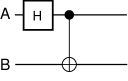
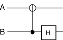
Figure 1: Circuits representing the coin operation of a Pavlov vs. Random quantum game. Left: Alice plays Random and Bob responds with Pavlov. Right: Alice plays Pavlov and Bob plays Random. These circuits map computational basis states into maximally entangled (Bell) states.

III.2 Sequential games

According to rule (ii) above, the quantum strategies available to Alice in a sequential game, are represented by unitary operations of the form  (6) affecting only the first qubit. The relation with a classical strategy, defined by four real parameters $[p_{R},p_{S},p_{T},p_{P}]$ with $p_{i}\in[0,1]$, is made explicit with the parametrization

$$\begin{array}[]{lcl}a_{0}=e^{i\varphi_{R}}\sqrt{p_{R}}&&a_{1}=e^{i\theta_{R}}\sqrt{1-p_{R}}\\ a_{2}=e^{i\varphi_{S}}\sqrt{p_{S}}&&a_{3}=e^{i\theta_{S}}\sqrt{1-p_{S}}\\ a_{4}=e^{i\varphi_{T}}\sqrt{p_{T}}&&a_{5}=e^{i\theta_{T}}\sqrt{1-p_{T}}\\ a_{6}=e^{i\varphi_{P}}\sqrt{p_{P}}&&a_{7}=e^{i\theta_{P}}\sqrt{1-p_{P}}\end{array}$$ (8)

where the phases $\varphi_{i},\theta_{i}\in[-\pi,\pi]$. A similar parametrization holds for the coefficients $b_{i}$ in eq. (7). Unitarity implies (aside from two conditions relating the phases) that

$$p_{R}+p_{T}=p_{S}+p_{P}=1.$$ (9)

Only classical strategies satisfying eq. (9) can be implemented as unitary operations in sequential quantum games. Each of these gives rise to a “family” of related quantum strategies. Aside from a global phase, a given sequential quantum strategy is determined by up to seven real parameters. Families of related strategies require fewer parameters however. For instance, quantum versions of Pavlov’s strategy as played by Alice, $[1,0,0,1]$, are implemented with operators of the form

$$U_{A}^{P}=|00\rangle\langle 00|+e^{i\nu_{1}}|11\rangle\langle 01|+e^{i\nu_{2}}|10\rangle\langle 10|+e^{i\nu_{3}}|01\rangle\langle 11|$$

in terms of three arbitrary phases $\nu_{j}$. If $\nu_{j}=0$, $U_{A}^{P}$ reduces to a controlled-NOT (CNOT) operation in which Bob’s coin is the control qubit N+C . Similarly, Pavlov’s strategies played by Bob are of the form

$$U_{B}^{P}=|00\rangle\langle 00|+e^{i\mu_{1}}|01\rangle\langle 01|+e^{i\mu_{2}}|11\rangle\langle 10|+e^{i\mu_{3}}|10\rangle\langle 11|,$$

and for $\mu_{j}=0$, they reduce to a CNOT operation controlled by Alice’s qubit. These are examples of conditional strategies, based on non-separable operators. Furthermore, since $[U_{A}^{P},U_{B}^{P}]\neq 0$, the order makes a difference when both players use Pavlov strategies.

ASan example of a separable strategy, consider the Hadamard operator $H$, defined by ${H|k\rangle=\frac{1}{\sqrt{2}}(|0\rangle+(-1)^{k}|1\rangle)}$ for $k=0,1$, which has been widely used as a coin operation in QW’s Kempe-review . In the context of QG’s, the fact that it generates unbiased superpositions of the computational basis states makes it useful as a quantum version of the classical Random strategy $\left[\frac{1}{2},\frac{1}{2},\frac{1}{2},\frac{1}{2}\right]$. A sequential quantum game in which Alice plays Pavlov and Bob replies with Random, is described, for a particular choice of phases, by a coin operation ${U_{c}=(I_{1}\otimes H)\cdot U_{A}^{P}}$, represented by the circuit in the right panel of Fig. 1.

An example with restricted strategic spaces

New outcomes are possible when quantum strategies are confronted. Consider a restricted strategic space in which ${p_{R}+p_{S}=1}$, so a players strategy is (aside from quantum phases) determined by a single angular parameter $\xi$ defined by $\cos^{2}\xi\equiv p_{R}$. For $\xi=0$ $(p_{R}=1)$ it reduces to Pavlov and for $\xi=\pi/4$, ${(p_{R}=0.5)}$ to Random. Values of $\xi\in[0,\pi/4]$ result in strategies which interpolate between Random and Pavlov. If the same parametrization is adopted for Bob’s strategy, the resulting two-parameter coin operation (assuming Alice plays first) is ${U_{c}=U_{B}(\xi_{B})\cdot U_{A}(\xi_{A})}$.

\psfrag{alpha}[1.5]{\vspace{2mm}\Huge$\xi_{A}$}\psfrag{beta}[1.5]{\Huge$\xi_{B}$}\psfrag{Payoff}[1.5]{\Huge$\bar{x}_{A,B}$}\psfrag{x0}[bl][1.3]{\Huge$~{}0$}\psfrag{xps4}[bl][1.3]{\Huge$~{}\frac{\pi}{4}$}\psfrag{y0}[bl][1.3]{\Huge$0\quad$}\psfrag{yps4}[bl][1.3]{\Huge$\frac{\pi}{4}\quad$}\includegraphics[angle={-90}]{./fig/ab-s1234c.ps}

\psfrag{alpha}[1.5]{\vspace{2mm}\Huge$\xi_{A}$}\psfrag{beta}[1.5]{\Huge$\xi_{B}$}\psfrag{Payoff}[1.5]{\Huge$\bar{x}_{A,B}$}\psfrag{x0}[bl][1.3]{\Huge$~{}0$}\psfrag{xps4}[bl][1.3]{\Huge$~{}\frac{\pi}{4}$}\psfrag{y0}[bl][1.3]{\Huge$0\quad$}\psfrag{yps4}[bl][1.3]{\Huge$\frac{\pi}{4}\quad$}\includegraphics[angle={-90}]{./fig/ab-sbell00c.ps}

Figure 2: (color online) Alice’s (red) and Bob’s (blue) payoffs after $N=50$ steps as a function of the strategic choice parametrized by angles $\xi_{A,B}\in[0,\pi/4]$ defined by $\cos^{2}\xi\equiv p_{R}$ for each player. The surfaces correspond to two unbiased initial conditions (see text for details).

This surface, after $N=50$ iterations, is shown in Fig. 2 for two unbiased initial coin states: the product state ${(|00\rangle+i|01\rangle+i|10\rangle-|11\rangle)/2}$ (left panel) and the fully entangled state $(|00\rangle+|11\rangle$)/$\sqrt{2}$ (right panel). Our results are for a set of unbiased values of the parameters which fulfill the PD constrains, eq. (4), $R$=$-P$=1 and $T$=$-S$=2. These results show that the classical situation (a tie for unbiased initial conditions) is exceptional in the quantum case and in the quantum game different initial coin states result in very different outcomes.

It is illustrative to look at the payoff of one agent vs the payoff of the other $(\bar{x}_{A}$ vs. $\bar{x}_{B})$. In Fig. 3 we show the results for two different unbiased initial coin states, ${\left(|00\rangle+|11\rangle\right)/\sqrt{2}}$ and ${\left(|01\rangle+|10\rangle\right)/\sqrt{2}}$

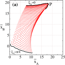
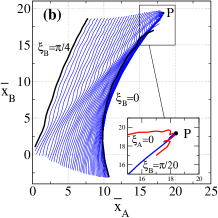
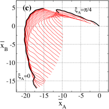
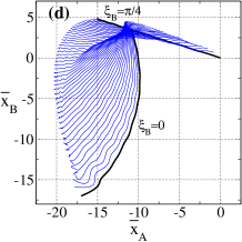
Figure 3: Average cumulated payoffs $(\bar{x}_{A}\mbox{ vs. }\bar{x}_{B})$ after $50$ iterations for different initial conditions. In panels (a,b) the initial coin is ${\left(|00\rangle+|11\rangle\right)/\sqrt{2}}$ and in panels (c,d) ${\left(|01\rangle+|10\rangle\right)/\sqrt{2}}$ Panels (a, c) show lines of constant $\xi_{A}$ (red online) and panels (b,d) show lines of constant $\xi_{B}$ (blue online). The extreme values of $\xi_{A}$ and $\xi_{B}$ are indicated by thick lines. In both cases, the other parameter ranges from $0$ (a Pavlovian strategy) to $\pi/4$ (a random strategy). The inset in panel (b) shows the lines for $\xi_{A}=0,\xi_{B}=\pi/20$ which intersect at the point P in which both agents maximize their average payoffs.

Note that, independently of Bob’s choice of strategy $\xi_{B}$, Alice must play Pavlov ($\xi_{A}=0$) in order to maximize her average return (see panel (a) ). Bob gets the highest average payoff when he adopts an intermediate strategy with ${\xi_{B}\simeq\pi/20}$, provided Alice plays Pavlov (see panel (b) ). In fact, this point ${(\xi_{A},\xi_{B})=(0,\pi/20)}$ is a Nash equilibrium which is also Pareto optimal (point P in the inset of Fig. 3b). As shown in panels (c,d), the same Pavlov strategy may result in a maximum or minimum payoff for Alice, depending on Bob’s choice of strategy.

As discussed above, not all classical strategies have quantum analogs in a sequential iterated quantum game. Clearly, playing always C (or D) is forbidden because it leads to non unitary operations. For the same reason, the TFT strategy is also forbidden in a sequential quantum game. However, if the strategic space is be extended by considering simultaneous moves of both players, this strategy becomes an option.

III.3 Simultaneous strategies

The case of simultaneous moves is closer to the classical situation and allows some new strategies to be implemented. Let $[p_{R}^{A},p_{S}^{A},p_{T}^{A},p_{P}^{A}]$ define the classical strategy to be implemented by Alice and $[p_{R}^{B},p_{S}^{B},p_{T}^{B},p_{P}^{B}]$ the one by Bob. A simultaneous quantum game confronting quantum versions of two these classical strategies involves unitary operations of the form,

$$\left[\begin{array}[]{cccc}e^{i\varphi_{11}}\sqrt{p_{R}^{A}p_{R}^{B}}&e^{i\varphi_{12}}\sqrt{p_{R}^{A}\bar{p}_{R}^{B}}&e^{i\varphi_{13}}\sqrt{\bar{p}_{R}^{A}p_{R}^{B}}&e^{i\varphi_{14}}\sqrt{\bar{p}_{R}^{A}\bar{p}_{R}^{B}}\\ e^{i\varphi_{21}}\sqrt{p_{S}^{A}p_{T}^{B}}&e^{i\varphi_{22}}\sqrt{p_{S}^{A}\bar{p}_{T}^{B}}&e^{i\varphi_{23}}\sqrt{\bar{p}_{S}^{A}p_{T}^{B}}&e^{i\varphi_{24}}\sqrt{\bar{p}_{S}^{A}\bar{p}_{T}^{B}}\\ e^{i\varphi_{31}}\sqrt{p_{T}^{A}p_{S}^{B}}&e^{i\varphi_{32}}\sqrt{p_{T}^{A}\bar{p}_{S}^{B}}&e^{i\varphi_{33}}\sqrt{\bar{p}_{T}^{A}p_{S}^{B}}&e^{i\varphi_{34}}\sqrt{\bar{p}_{T}^{A}\bar{p}_{S}^{B}}\\ e^{i\varphi_{41}}\sqrt{p_{P}^{A}p_{P}^{B}}&e^{i\varphi_{42}}\sqrt{p_{P}^{A}\bar{p}_{P}^{B}}&e^{i\varphi_{43}}\sqrt{\bar{p}_{P}^{A}p_{P}^{B}}&e^{i\varphi_{44}}\sqrt{\bar{p}_{P}^{A}\bar{p}_{P}^{B}}\end{array}\right]$$

where $e^{i\varphi_{kl}}$ are phase factors and $\bar{p}_{i}^{A,B}\equiv 1-p_{i}^{A,B}$. For a real $U_{c}$, $e^{i\varphi_{kl}}=\pm 1$, unitarity requires

$$(p_{R}^{A}-\bar{p}_{S}^{A})(p_{R}^{B}-\bar{p}_{T}^{B}) = (p_{R}^{A}-\bar{p}_{T}^{A})(p_{R}^{B}-\bar{p}_{S}^{B})=0,$$

$$(p_{R}^{A}-\bar{p}_{P}^{A})(p_{R}^{B}-\bar{p}_{P}^{B}) = (p_{S}^{A}-\bar{p}_{T}^{A})(p_{S}^{B}-\bar{p}_{T}^{B})=0,$$

$$(p_{S}^{A}-\bar{p}_{P}^{A})(p_{T}^{B}-\bar{p}_{P}^{B}) = (p_{T}^{A}-\bar{p}_{P}^{A})(p_{S}^{B}-\bar{p}_{P}^{B})=0.$$

In the general case, analogous restrictions involving the phases $\varphi_{kl}$ apply. For instance, the game in which Alice plays Pavlov $[1,0,0,1]$ and Bob simultaneously plays TFT $[1,0,1,0]$ is implemented by

$$U_{c}^{PT}=|00\rangle\langle 00|+e^{i\lambda_{1}}\!|10\rangle\langle 01|+e^{i\lambda_{2}}|11\rangle\langle 10|+e^{i\lambda_{3}}|01\rangle\langle 11|,$$

in terms of three arbitrary phases $\lambda_{i}$. In the classical version of this game, if both agents start playing C with probability $0.5$, after $N$ iterations each collects a null average payoff $N(R+P)=0$. In the quantum game with the above mentioned Bell state as initial condition, the winning chances are not equal and both players end up with positive payoffs. In a similar way, other classical strategies may be confronted. The simultaneous scheme is closer to classical games but it is limited by conditions (III.3). For example, if both players adopt Pavlov, they cannot play simultaneously, as some of these conditions are not satisfied. In Table I, we consider three classical strategies and indicate which of them can be confronted within the quantum sequential and/or simultaneous schemes. Games confronting TFT vs Random may be described by (non-unitary) quantum operations. We do not consider these extensions in this work.

	Random	Pavlov	TFT
Random	1, 2	1,2	not unitary
Pavlov	1,2	1	2
TFT	not unitary	2	2

Table 1: Some strategies that can be confronted both in sequential (1) and simultaneous (2) quantum games.

IV Concluding Remarks

We have related general bi-partite iterated quantum games to discrete time quantum walks. Several strategies from classical game theory can be implemented in terms of elementary two-qubit quantum gates. Each of them gives rise to a family of quantum strategies. We give the conditions that must be satisfied so that two classical strategies may be confronted, either sequentially or simultaneously, in an interated quantum game. Some well-known classical strategies, such as TFT can only be implemented in the simultaneous scheme. Non-conmuting operations, such as those associated to a Pavlov-Pavlov confrontation, can only be realized in the sequential scheme. Since the parameter space for these quantum strategies is extremely large, instead of a systematic exploration, we have shown through selected examples that the outcome of a QG may be different from that of the classical counterpart.

In one-shot quantum games, there is a threshold for the amount of entanglement in the initial state that allows quantum features to emerge Eisert99 ; Du03 . In our proposal, entanglement is dynamically generated by conditional operations and the preparation of an initially entangled state is not required. We have characterized the bi-partite entanglement between both agents in a Pavlov-Random QG using the von Neumann entropy of the reduced density operator (entropy of entanglement) and found that this quantity increases at a logarithmic rate. In order to exploit entanglement partial measurements may be included as part of the strategic choices.

The connection between bipartite quantum games and discrete-time quantum walks opens the possibility of experimentally testing iterated quantum games and strategies using simple linear optics elements Do . The sensitivity of these QGs to the choice of the initial state may be attenuated in experimental realizations through the introduction of decoherence. The impact of a weak coupling to the environment is a relevant issue in the study of quantum games, which deserves further study, as, in the classical case, noise-related effects are able to radically change the outcome of the different strategies Nowak . An initial step in this direction may be considering the outcome, for different strategic options, of opposing a classical player vs. a quantum player.

The scheme we have introduced for quantizing the iterated PD game can obviously be applied to $2\times 2$ games with an arbitrary payoff matrix. There are several popular games that seem interesting to analyze within this framework. For example the Hawk-Dove ms82 , in which the damage from mutual defection in the PD is increased so that it finally exceeds the damage suffered by being exploited: $T>R>S>P$. Or the Stag Hunt game s04 , corresponding to the payoffs rank order $R>T>P>S$ i.e. when the reward $R$ for mutual cooperation in the PD games surpasses the temptation $T$ to defect.

Another generalization of this scheme involves multi-partite games. The basic evolution, given by eqs. (1) and (2), may be generalized to accomodate any number of quantum walkers. This may be useful for the ”public goods“ problem, since there are indications that the quantum version of this multiplayer game may provide a more efficient distribution of resources ChenHogg06 . However, this generalization raises non-trivial issues regarding the multipartite entanglement which may be dynamically generated within the game.

Aknowledgements

Work supported by PEDECIBA and PDT project 29/84 (Uruguay), CNPq and FAPERJ (Brazil).

References

- (1) J. Kempe, Contemporary Physics, 44:307 (2003); e-print quant-ph/0303081.
- (2) J. Kempe, Probability Theory, 133:215 (2005); e-print quant-ph/0205083.
- (3) N. Shenvi, et al., Phys. Rev. A 67:052307 (2003); e-print quant-ph/0210064.
- (4) A.M. Childs et al., Proc. 35th ACM Symp. on Theory of Computing (STOC 2003) p. 59 (2003); e-print quant-ph/0209131.
- (5) E. Fahri, J. Goldstone and S. Gutmann, A Quantum algorithm for the Hamiltonian NAND tree, e-print quant-ph/0702144.
- (6) C.A. Ryan et al., Phys. Rev. A 72:062317 (2005).
- (7) B. Do et al., J. Opt. Soc. Am. B 22:499 (2005).
- (8) D.A. Meyer, Phys. Rev. Lett. 82:1052 (1999).
- (9) J. Eisert, M. Wilkens, M. Lewenstein, Phys. Rev. Lett. 83:3077 (1999).
- (10) A. Iqbal and A. H. Toor, Phys. Lett. A 300541 (2002).
- (11) C. F. Lee and N.F. Johnson, Phys. Rev. A 67:022311 (2003).
- (12) H. Du et al., Fluct. Noise Lett., 2:R189 (2002); e-print quant-ph/0301042.
- (13) N. Patel, Nature 445:144 (2007)
- (14) K. Chen and T. Hogg, Quant. Inf. Proc. 1:449 (2003); e-print quant-ph/0301013.
- (15) K. Chen and T. Hogg, Quant. Inf. Proc. 5:43 (2006).
- (16) G. Abal et al., Phys. Rev. A 73:042302 (2006) and 069905(E) (2006) ; e-print quant-ph/0507264.
- (17) Y. Omar, N. Paunkovic, L. Sheridan, S. Bose, Phys. Rev. A 74:042304 (2006) ; S.E. Venegas-Andraca et al., New J. Phys. 7:221 (2005).
- (18) M. Flood, Some Experimental Games, Research Memorandum, RM-789 , RAND Corporation, June 1952.
- (19) D. Kraines and V. Kraines, Theory Decision 26:47 (1989).
- (20) M.A. Nielsen and I.L. Chuang, Quantum Computation and Quantum Information, Cambridge University Press, 2000.
- (21) M.A. Nowak and K. Sigmund, Nature 364:56 (1993).
- (22) J. Maynard-Smith, Evolution and the Theory of Games, Cambridge Univ. Press 1982.
- (23) B. Skyrms, The Stag Hunt and the Evolution of Social Structure, Cambridge University Press 2004.