Experimental Long-Distance Decoy-State Quantum Key Distribution Based On Polarization Encoding

Abstract

We demonstrate the decoy-state quantum key distribution (QKD) with one-way quantum communication in polarization space over 102 km. Further, we simplify the experimental setup and use only one detector to implement the one-way decoy-state QKD over 75 km, with the advantage to overcome the security loopholes due to the efficiency mismatch of detectors. Our experimental implementation can really offer the unconditionally secure final keys. We use 3 different intensities of 0, 0.2 and 0.6 for the light sources in our experiment. In order to eliminate the influences of polarization mode dispersion in the long-distance single-mode optical fiber, an automatic polarization compensation system is utilized to implement the active compensation.

Quantum key distribution BB84 ; GRTZ02 ; DLH06 can in principle offer the unconditionally secure private communications between two remote parties, Alice and Bob. However, the security proofs for the ideal BB84 protocol M01 ; SP00 do not guarantee the security of a specific setup in practice due to various imperfections there. One important problem in practical QKD is the effects of the imperfect source, say, the coherent states. The decoy state method H03 ; Wang05 ; Wang05_2 ; LMC05 ; HQph or some other methods SARG04 ; K04 can help to generate the unconditionally secure final keys even an imperfect source is used by Alice in practical QKD. Basically, QKD can be realized in both free space and optical fiber GRTZ02 . Each option has its own advantages. The fiber QKD can be run in the always-on mode: it runs in both day and night and is not affected by the weather. Also, the future local QKD networks are supposed to be using fiber. So far, there are many experiments of fiber QKD with weak coherent lights QKD . However, these results actually do not offer the unconditional security because of the possible photon-number-splitting attack PNS . Recently, there are also experimental implementations of the decoy-state method Lo06 , with two-way quantum communication. However, since these implementations have not taken the specific operations as requested by Ref. GFKZR05 , the security of the final keys is still unclear due to the so-called Trojan horse attacks GRTZ02 . One can implement active counter-measures GFKZR05 to overcome this problem, which is deserved experimental implementations in the future. The other way is to use one-way quantum communication which we have adopted in this work.

Here we present the first polarization-based decoy-state QKD implementation over 102 km with only one-way quantum communication using two detectors and 75 km using only one detector. Our results are unconditionally secure (For the unconditional security, we mean that the probability that Eve has non-negligible amount of information about the final key is exponentially close to 0, say, $e^{-O(100)}$). Here we must clarify that given the existing technologies QKD , if the distance is shorter than about 20 km, through the simple worst-case estimation GLLP04 of the fraction of tagged bits it is still possible for one to implement the unconditionally secure QKD without using the decoy-state method.

We can know how to distill the secure final keys with imperfect source given the separate theoretical results from Ref. GLLP04 , if we know the upper bound of the fraction of tagged bits (those raw bits generated by multi-photon pulses from Alice) or equivalently, the lower bound of the fraction of untagged bits (those raw bits generated by single-photon pulses from Alice). In Wang’s 3-intensity decoy-state protocol Wang05 ; Wang05_2 , one can randomly use 3 different intensities (average photon numbers) of each pulses (0, $\mu$, $\mu^{\prime}$) and then observe the counting rates (the counting probability of Bob’s detector whenever Alice sends out a state) of pulses of each intensities ($S_{0},S_{\mu},S_{\mu^{\prime}}$). The density operators for the states of $\mu$ and $\mu^{\prime}$ ($\mu^{\prime}>\mu$) are

$$\left\{\begin{array}[]{ll}\rho_{\mu}=e^{-\mu}|0\rangle\langle 0|+\mu e^{-\mu}|1\rangle\langle 1|+c\rho_{c}\\ \rho_{\mu^{\prime}}=e^{-\mu^{\prime}}|0\rangle\langle 0|+\mu^{\prime}e^{-\mu^{\prime}}|1\rangle\langle 1|+\frac{\mu^{\prime 2}e^{-\mu^{\prime}}}{\mu^{2}e^{-\mu}}c\rho_{c}+d\rho_{d},\end{array}\right.$$ (3)

here $c={1-e^{-\mu}-\mu e^{-\mu}}$,$\rho_{c}=\frac{e^{-\mu}}{c}\sum_{n=2}^{\infty}\frac{\mu^{n}}{n!}|n\rangle\langle n|$, $\rho_{d}$ is a density operator and $d>0$ (here we use the same notations in Ref. Wang05 ; Wang05_2 ). We denote $s_{0}(s_{0}^{\prime}),s_{1}(s_{1}^{\prime}),s_{c}(s_{c}^{\prime})$ for the counting rates of those vacuum pulses, single-photon pulses and $\rho_{c}$ pulses from $\rho_{\mu}(\rho_{\mu^{\prime}})$. Asymptotically, the values of primed symbols here should be equal to those values of unprimed symbols. However, in an experiment the number of samples is finite therefore they could be a bit different. The bound values of $s_{1},s_{1}^{\prime}$ can be determined by the following joint constraints corresponding to Eq.(15) of Ref. Wang05_2

$$\left\{\begin{array}[]{ll}S_{\mu}=e^{-\mu}s_{0}+\mu e^{-\mu}s_{1}+cs_{c}\\ cs_{c}^{\prime}\leq\frac{\mu^{2}e^{-\mu}}{\mu^{\prime 2}e^{-\mu^{\prime}}}(S_{\mu^{\prime}}-\mu^{\prime}e^{-\mu^{\prime}}s_{1}^{\prime}-e^{-\mu^{\prime}}s_{0}^{\prime}),\end{array}\right.$$ (6)

where $s_{1}^{\prime}=(1-\frac{10e^{\mu/2}}{\sqrt{\mu s_{1}N_{\mu}}})s_{1}$, $s_{c}^{\prime}=(1-\frac{10}{\sqrt{s_{c}N_{\mu}}})s_{c}$, $s_{0}^{\prime}=0$, $s_{0}=(1+r_{0})S_{0}$ and $r_{0}=\frac{10}{\sqrt{S_{0}N_{0}}}$ to obtain the worst-case results Wang05 ; Wang05_2 . $N_{\mu},N_{0}$ are the pulse numbers of intensity $\mu,0$. Given these, one can calculate $s_{1},s_{1}^{\prime},s_{c}$ numerically.

The experimental setup is shown in Fig.1, mainly including transmitter (Alice), quantum channel, receiver (Bob) and electronics system. All the electronics modules are designed by ourselves. The synchrodyne (SD) is designed by field programmable gate array (FPGA, Altera Co.) and outputs multiple channels of synchronous clocks with independent programmable parameter settings, which is equivalent to an arbitrary function generator, to drive the modules of random number generator (RNG), data acquisition (DAQ, designed by FPGA) and single-photon detector (SPD) respectively. The signals with FWHM of about 1 ns are generated by laser diode driver (LDD) to drive 10 distributed feed-back laser diodes (LD) at the central wavelength of 1550 nm, where 4 LDs are used for decoy states ($\mu$) and another 4 LDs are used for signal states ($\mu^{\prime}$) and the other 2 LDs are used for polarization calibration. The polarization states of photons emitting from LDs can be transformed to arbitrary polarization state by polarization controller (PC). For decoy states and signal states, the four polarization states are $|H\rangle,|V\rangle,|+\rangle,|-\rangle$, where $|H\rangle,|V\rangle$ represent horizontal polarization and vertical polarization, $|+\rangle=1/\sqrt{2}(|H\rangle+|V\rangle)$ and $|-\rangle=1/\sqrt{2}(|H\rangle-|V\rangle)$, as the four states for the standard BB84 protocol BB84 . For test states, the two polarization states are $|H\rangle$ and $|+\rangle$ to calibrate the two sets of polarization basis. The photons of every channel are coupled to an optical fiber via fiber coupling network (FCN), which is composed of multiple beam splitters (BS) and polarization beam splitters (PBS) and optical attenuators. In FCN, the fiber length of every channel must be adjusted precisely so that the arrival time differences to SPD caused by the fiber length differences can be less than 100 ps.

In the setup, a dense wavelength division multiplexing fiber filter (FF) is inserted in Alice’s side. On the one hand, it can guarantee that the wavelengths of emitted photons in all channels are equal to avoid the possibility of Eve’s attack utilizing the variance of photon wavelengths. On the other hand, it can reduce the influences of chromatic dispersion in fiber.

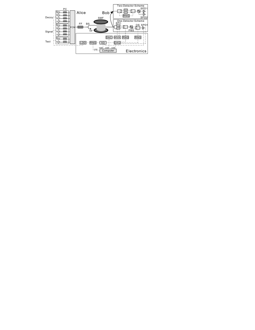
Figure 1: Schematic diagram of the experimental setup. Solid line and dashed line represent optical fiber and electric cable respectively. See the text for the abbreviations.

In the experiment, the pulse numbers ratio of the 3 intensities is $5:4:1$ and the intensities of signal states and decoy states are fixed at $\mu^{\prime}=0.6$ and $\mu=0.2$ respectively, which are not necessarily the optimized parameters with our setup. The fluctuations of intensities are monitored at the test point (TP). If the varying range of fluctuation is larger than about 5% we will stop the system and adjust the light sources. In fact, the effects of intensity fluctuation is indeed a very important theoretical problem for the decoy-state QKD, which had not been solved by theorists prior to our experiment. Very recently theoretical progress has shown that the effects are moderate with certain modifications of the experimental setup Wang06 .

After passing through the long-distance single-mode fiber (SMF, Corning Co., fiber attenuation is about 0.2 dB/km), at Bob’s side we adopt two kinds of measurement scheme. In one-detector scheme, firstly a fiber BS is used to select the two polarization basis called $HV$ basis and $+-$ basis randomly. Secondly due to the polarization mode dispersion (PMD) effects in long-distance SMF, we develop an automatic polarization compensation (APC) system to compensate for the PMD actively. The principles of APC are: Alice sends fixed $|H\rangle$ states or $|+\rangle$ states. Then Bob records the accepted counting rates in the corresponding basis using DAQ system and transmits them to the computer via universal serial bus (USB). After algorithmic processing, the computer gives out the data, which can be converted to voltages of electric polarization controllers (EPC, General Photonics Co.) through digital-to-analog converter (DAC) and high voltage amplifier (HVA). Then the fiber squeezers in EPC are driven by the voltages and change the polarization EPC . After repeating feedback controls the visibility of test states can reach the target value and the APC system stops. The average adjusting time is about 3 minutes. However, this time can be greatly shortened using a continuous coherent light and wavelength division multiplexing techniques and optimized algorithms. Figure 2(a) shows the test results of the APC system with 75 km fiber. In the experiment, Alice starts APC to calibrate the system first. After calibration she transmits the pulses for several minutes. Then this process is repeated. Thirdly we use two magnetic optical switch (OS, Primanex Co.) with switching time of less than 20 $\mu s$ driven by two independent RNG to randomly switch the basis and the output ports of PBS respectively. The one-detector scheme can overcome the security loopholes due to the efficiency mismatch of detectors TSA since the fiber lengths of each state can be adjusted identically. On the other hand, two OS driven by the same RNG and two SPDs Note1 are used in two-detector scheme to reduce the transmission losses in Bob’s side.

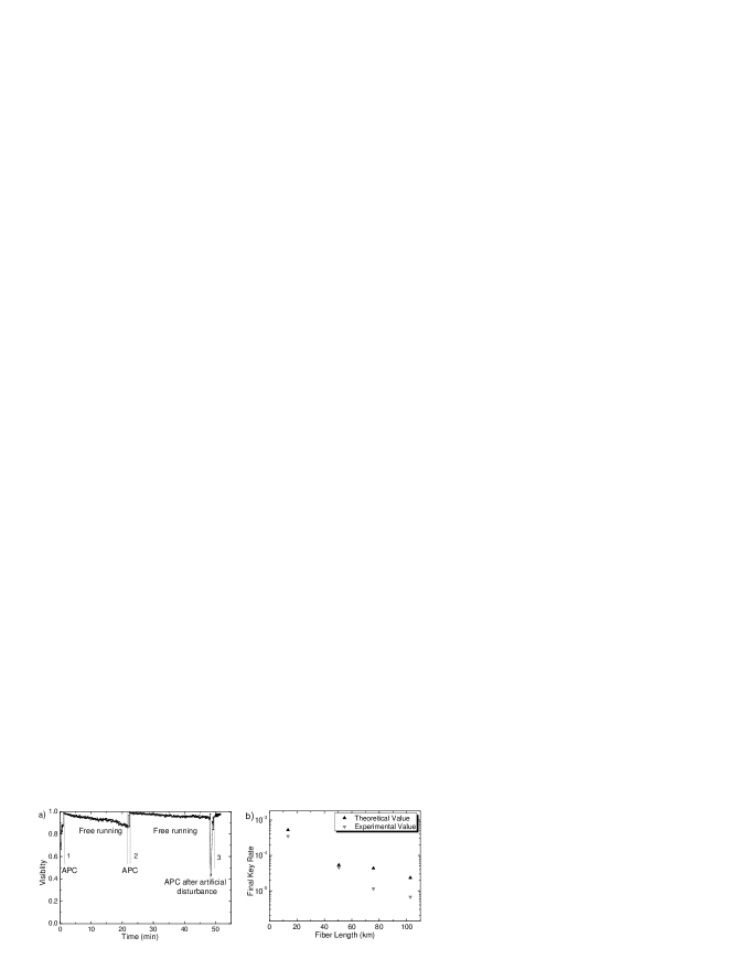
Figure 2: a) Test of the APC system with 75 km fiber. In position 1 and 2 the APC system monitors the visibility changes of polarization states and adjusts the voltages of EPC actively to reach the target visibility. Subsequently, the visibility of polarization states becomes worse slowly when free running. In position 3, artificial disturbance induces drastic change of visibility and the APC system can still work well. The time interval of points is 2 seconds. b) Comparison of the final key rate of signal states per pulse between the theoretical calculation and experimental results with four different distance settings $L$ (13.448 km, 50.524 km, 75.774 km and 102.714 km), where their corresponding total attenuations are (24.9 dB, 32.2 dB, 34.8 dB, 37.0 dB) including channel losses, all the insertion losses of components, detector efficiencies etc. The first three settings use one-detector scheme and the last one uses two-detector scheme. The first two settings’ repetition frequency is $f$=4 MHz and the last two is $f$=2.5 MHz.

We use this all-fiber quantum cryptosystem to implement the decoy-state QKD over 102 km and 75 km using two-detector scheme and one-detector scheme respectively. The experimental parameters and their corresponding values are listed in Table 1. In the experiment, Alice totally transmits about $N$ pulses to Bob. After the transmission Bob announces the pulse sequence numbers and basis information of received states. Then Alice broadcasts to Bob the actual state class information and basis information of the corresponding pulses. Alice and Bob can calculate the experimentally observed quantum bit error rate (QBER) values $E_{\mu},E_{\mu^{\prime}}$ of decoy states and signal states according to all the decoy bits and a small fraction of the signal bits respectively Note2 .

Table 1: Experimental parameters (P.) and their corresponding values of 75.774 km (Value1) and 102.714 km (Value2) decoy-state QKD.

P.	Value1	Value2	P.	Value1	Value2
$L$	75.774 km	102.714 km	$S_{\mu^{\prime}}$	$2.076\times 10^{-4}$	$1.262\times 10^{-4}$
$f$	2.5 MHz	2.5 MHz	$S_{\mu}$	$7.534\times 10^{-5}$	$4.611\times 10^{-5}$
$N$	$1.607\times 10^{9}$	$5.222\times 10^{9}$	$S_{0}$	$9.174\times 10^{-6}$	$6.711\times 10^{-6}$
$E_{\mu^{\prime}}$	3.231%	3.580%	$s_{1}^{\prime}$	$2.460\times 10^{-4}$	$1.558\times 10^{-4}$
$E_{\mu}$	9.039%	9.098%	$R_{\mu^{\prime}}$	$1.143\times 10^{-5}$	$6.706\times 10^{-6}$
$E_{1}^{\mu^{\prime}}$	6.099%	5.854%	$R_{E}$	11.668 Hz	8.090 Hz
$R_{T}$	46.167 Hz	29.427 Hz	$\frac{R_{E}}{R_{T}}$	0.253	0.275

Then we can numerically calculate a tight lower bound of the counting rate of single-photon $s_{1}^{\prime}$ using Eq. 6. The next step is to estimate the fraction of single-photon $\Delta_{1}$ and the QBER upper bound of single-photon $E_{1}$. We use

$$\Delta_{1}^{\mu^{\prime}}=s_{1}^{\prime}\mu^{\prime}e^{-\mu^{\prime}}/S_{\mu^{\prime}},\Delta_{1}^{\mu}=s_{1}\mu e^{-\mu}/S_{\mu}$$ (7)

to conservatively calculate $\Delta_{1}$ of signal states and decoy states respectively Wang05 ; Wang05_2 . And $E_{1}$ of signal states and decoy states can be estimated by the following formula,

$$E_{1}^{\mu^{\prime}(\mu)}=(E_{\mu^{\prime}(\mu)}-\frac{(1-r_{0})S_{0}e^{-\mu^{\prime}(\mu)}}{2S_{\mu^{\prime}(\mu)}})/\Delta_{1}^{\mu^{\prime}(\mu)}.$$ (8)

Here we consider the statistical fluctuations of the vacuum states to obtain the worst-case results.

Lastly we can calculate the final key rates of signal states using the formula Wang05 ; Wang05_2 of

$$R_{\mu^{\prime}}=S_{\mu^{\prime}}(\Delta_{1}^{\mu^{\prime}}-H(E_{\mu^{\prime}})-\Delta_{1}^{\mu^{\prime}}H(E_{1}^{\mu^{\prime}})),$$ (9)

here $H(x)=-xlog_{2}(x)-(1-x)log_{2}(1-x)$. Then we compare the experimental final key rate of signal states $R_{E}$ with the theoretically allowed value $R_{T}$, i.e., in the case both $\Delta_{1}$ and $E_{1}$ are known without any overestimation. The theoretically allowed values of $\Delta_{1}$ and $E_{1}$ for signal states are

$$\left\{\begin{array}[]{ll}\Delta_{1T}^{\mu^{\prime}}=(S_{\mu^{\prime}}-(1-\mu^{\prime})S_{0})e^{-\mu^{\prime}}/S_{\mu^{\prime}}\\ E_{1T}^{\mu^{\prime}}=(E_{\mu^{\prime}}-\frac{S_{0}e^{-\mu^{\prime}}}{2S_{\mu^{\prime}}})/\Delta_{1T}^{\mu^{\prime}},\end{array}\right.$$ (12)

with the assumptions that the ideal value of the single-photon counting rate is $s_{1T}=\eta+S_{0}$ and $S_{\mu^{\prime}}=\eta\mu^{\prime}+S_{0}$, where $\eta$ is the overall transmittance. We find out that our experimental results in the two cases are both close to 30% of the theoretically allowed maximum value.

During the above calculation, we have used the worst-case results in every step for the security. Obviously, there are more economic methods for the calculation of final key rate. Here we have not considered the consumption of raw keys for QBER test. Now we reconsider the key rate calculation of decoy states above. We assumed the worst case of $s_{0}=(1+r_{0})S_{0}$ and $s_{0}=(1-r_{0})S_{0}$ for calculating $\Delta_{1}^{\mu}$ and $E_{1}^{\mu}$ respectively. Although we don’t exactly know the true value of $s_{0}$, there must be one fixed value for both calculations. Therefore we can choose every possible value in the range of $(1-r_{0})S_{0}\leq s_{0}\leq(1+r_{0})S_{0}$ and use it to calculate $\Delta_{1}^{\mu}$, $E_{1}^{\mu}$ and the final key rate, and then pick out the smallest value as the lower bound of decoy states key rate. Figure 3 demonstrates the results with a larger range of $|r_{0}|$ ($r_{0}$ can be negative here) than the actual range in the case of 13.448 km. This economic calculation method can obtain a more tightened value of the lower bound, which is larger than the result using the simple calculation method above with two-step worst-case assumption for $s_{0}$ values.

We have tested the system with different fiber lengths and compared the final key rates with the theoretical values, see Fig.2(b). The differences between them are mainly due to the imperfect polarization compensation and the possible statistical fluctuation.

Figure 3: The final key rate of decoy pulses varies with the vacuum counting rate of $s_{0}$ in the case of 13.448 km, where $s_{0}=(1+r_{0})S_{0}$.

The two measurement schemes have their own advantages. One-detector scheme can overcome the security loopholes of the detector efficiency mismatch and generate the unconditionally secure final keys while the other can implement longer distance. If we use four-detector scheme with four high quality SPDs the final key rate and maximum distance will be improved. Also, the balance between the efficiency and the dark counts of SPD is important. During the experiment, we have even reduced the efficiency of SPD purposely to reduce the dark counts to obtain better balance. Hopefully, a low-noise and high-efficiency detector at telecommunication wavelengths can be used in the future to further improve the final key rate. The superconducting transition-edge sensor is one of the promising candidates TES .

In summary, we implement the polarization-based one-way decoy-state QKD over 102 km and also implement 75 km one-way decoy-state QKD using only one detector to really offer the unconditionally secure final keys.

This work is supported by the NNSF of China, the CAS and the National Fundamental Research Program.

References

- (1) C.H. Bennett and G. Brassard, in Proc. of IEEE Int. Conf. on Computers, Systems, and Signal Processing (IEEE, New York, 1984), pp. 175-179.
- (2) N. Gisin, G. Ribordy, W. Tittel, and H. Zbinden, Rev. Mod. Phys. 74, 145 (2002).
- (3) M. Dusek, N. Lütkenhaus, M. Hendrych, in Progress in Optics VVVX, edited by E. Wolf (Elsevier, 2006).
- (4) D. Mayers, J. ACM 48, 351 (2001).
- (5) P. W. Shor and J. Preskill, Phys. Rev. Lett. 85, 441 (2000).
- (6) W.-Y. Hwang, Phys. Rev. Lett. 91, 057901 (2003).
- (7) X.-B. Wang, Phys. Rev. Lett. 94, 230503 (2005).
- (8) X.-B. Wang, Phys. Rev. A 72, 012322 (2005).
- (9) H.-K. Lo, X. Ma, and K. Chen, Phys. Rev. Lett. 94, 230504 (2005); X. Ma et al., Phys. Rev. A 72, 012326 (2005).
- (10) J.W. Harrington et al., quant-ph/0503002.
- (11) V. Scarani et al., Phys. Rev. Lett. 92, 057901 (2004); C. Branciard et al., Phys. Rev. A 72, 032301 (2005).
- (12) M. Koashi, Phys. Rev. Lett. 93, 120501(2004); K. Tamaki, et al., quant-ph/0607082.
- (13) M. Bourennane et al., Opt. Express 4, 383 (1999); D. Stucki et al., New. J. Physics, 4, 41, (2002); H. Kosaka et al., Electron. Lett. 39, 1199 (2003); C. Gobby, Z.L. Yuan, and A.J. Shields, Appl. Phys. Lett. 84, 3762 (2004); X.-F Mo et al., Opt. Lett. 30, 2632 (2005).
- (14) B. Huttner et al., Phys. Rev. A 51, 1863 (1995); H.P. Yuen, Quantum Semiclassic. Opt. 8, 939 (1996); G. Brassard et al., Phys. Rev. Lett. 85, 1330 (2000); N. Lütkenhaus, Phys. Rev. A 61, 052304 (2000); N. Lütkenhaus and M. Jahma, New J. Phys. 4, 44 (2002).
- (15) Y. Zhao et al., Phys. Rev. Lett. 96, 070502 (2006); Y. Zhao et al., quant-ph/0601168.
- (16) N. Gisin et al., Phys. Rev. A 73, 022320 (2006).
- (17) H. Inamori, N. Lütkenhaus, D. Mayers, quant-ph/0107017; D. Gottesman, H.-K. Lo, N. Lütkenhaus, and J. Preskill, Quantum Inf. Comput. 4, 325 (2004).
- (18) X.-B. Wang, quant-ph/0609081; X.-B. Wang, C.-Z. Peng, quant-ph/0609137.
- (19) R. Noé, Electron. Lett. 22, 772-773 (1986); N. G. Walker and G. R. Walker, Electron. Lett. 23, 290-292 (1987); R. Noé, H. Heidrich, and D. Hoffmann, J. Lightwave Technol. 6, 1199-1207 (1988).
- (20) V. Makarov, A. Anisimov, J. Skaar, Phys. Rev. A 74, 022313 (2006); B. Qi et al., quant-ph/0512080.
- (21) Detection efficiency , , the timing windows are both 2.5 ns, and the dark count rates are about /pulse and /pulse respectively. The actual observed value of is larger than these parameters due to the imperfect light sources.
- (22) Like other papers, e.g., Ref Lo06 , the treatment of QBER here is simple. However, we can use stricter calculation methods. For instance, we use all the basis bits for testing the phase flip error and 10% of basis bits for testing bit flip error, while in estimating the phase flip and bit flip error rate for the remaining basis bits we use 10 standard deviations and 1 standard deviation, respectively. And a factor of should be multiplied to calculate the final key rate. Even applying this strict way we can still obtain positive final keys with thousands of final bits from our experiment in the case of 102.714 km.
- (23) K.D. Irwin, Appl. Phys. Lett. 66, 1998 (1995); B. Cabrera et al., Appl. Phys. Lett. 73, 735 (1998); D. Rosenberg et al., Phys. Rev. A 71, 061803(R) (2005).