Quantum heat engine with continuum working medium

Abstract

We introduce a new quantum heat engine, in which the working medium is a quantum system with a discrete level and a continuum. Net work done by this engine is calculated and discussed. The results show that this quantum heat engine behaves like the two-level quantum heat engine in both the high-temperature and the low-temperature limits, but it operates differently in temperatures between them. The efficiency of this quantum heat engine is also presented and discussed.

A classical heat engine converts heat energy into mechanical work by using a classical-mechanical system in which a working medium(for example, a gas) expands and pushes a piston in a cylinder. Working between a high-temperature reservoir and a low-temperature reservoir, the classical heat engine achieves maximum efficiency when it is reversible, while the efficiency is zero if the two reservoirs have the same temperature. The situation changes for its quantum counterpart, where the working medium and the dynamics that govern the cycle are quantum. It was shown that the quantum heat engine can better the work extraction and improve the engine efficiencyscully03 ; kieu03 ; kieu04 ; quan05 ; quan05p .

The quantum heat engine concept was introduced by Scovil and Schultz-Dubois scovil59 and extended in many later workslloyd97 ; kosloff00 ; scully03 ; kieu03 ; kieu04 ; quan05 ; quan05p . Quantum heat engines are characterized by three attributes: the working medium, the cycle of operation, and the dynamics that govern the cycle. In the previous works, the working medium is considered as an ensemble of many non-interacting discrete level systems. Specifically, the analysis is carried out on two-level systemskieu03 ; feldmann00 , three-level systemsquan05 , as well as an ensemble of harmonic oscillatorskieu03 ; feldmann96 ; bender01 . These give rise to the following questions, with continuum working medium what is the work extraction of quantum heat engine? Can such a quantum heat engine improve the work extraction?

In this paper we will answer these questions by examining an quantum heat engine working between two reservoirs with different temperatures. The working medium is envisioned as a quantum system with a discrete level $|d\rangle$ and a continuum $|c\rangle$ as shown in figure 1.

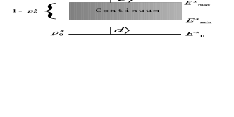
Figure 1: An illustration of the level structure of the working medium. The occupation probability $p_{0}^{x},x=l,h$ of the discrete level $|d\rangle$ (with eigenenergy $E_{0}^{x}$) was kept fixed in adiabatic processes. The continuum broadening was denoted by $E_{max}^{x}-E_{min}^{x}$ .

Non-interacting Ba atoms, for example, may serve as the quantum systemnoordam92 , in which the bound coherent Rydberg state $6s(n+2)d$ might be taken as the discrete level. The heat-engine cycle consists of four branches labelled by 1,2,3 and 4, this was schematically illustrated in figure 2.

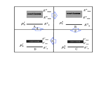
Figure 2: Schematic illustration of the four-stroke quantum heat engine. From state A to B, the working medium absorbs heat from the high-temperature reservoir, leading to population transfer from the discrete level $|d\rangle$ to the continuum. From state B to C, works are done with the working medium undergoing an adiabatic process. The Branches 3 and 4(corresponding changes from C to D, and from D to A, respectively.) are reversed processes of 1 and 2, respectively. We will use $(E_{0}^{x},E_{min}^{x},E_{max}^{x})$ to characterize the level structure of the working medium in the text.

This four-stroke quantum heat engine is a quantum analogue of the classical Otto engine, which includes two quantum adiabatic processes (2 and 4) and two isothermal processes (1 and 3).

Denoting $p_{0}^{x},$ ${x=h,l}$ the occupation probability of the discrete level and $p(E)$ the occupation probability of the continuum, we can write the expectation value of the measured energy of a quantum system $U$ as,

$$U=\langle E\rangle=\sum_{i}p_{i}E_{i}+\int d[p(E)\cdot E].$$ (1)

The definition of infinitesimal work done in a process is then

$${\mathchar 22\relax\mkern-11.0mud}W=\sum_{i}p_{i}dE_{i}+\sum^{E_{max}}_{E_{min}}p(E)dE,$$ (2)

which is a straightforward extension of that for discrete level systemsfeldmann00 to the system under our consideration. The first term comes from the contribution of discrete levels, while the last term comes from the continuum. By the first law of thermodynamics $dU={\mathchar 22\relax\mkern-11.0mud}Q+{\mathchar 22\relax\mkern-11.0mud}W$, the infinitesimal heat absorbed is

$${\mathchar 22\relax\mkern-11.0mud}Q=\sum_{i}E_{i}dp_{i}+\sum^{E_{max}}_{E_{min}}Edp(E).$$ (3)

With these notations, we now calculate the work done on the four branches of the heat engine.

In the branch 1, namely, from A to B, the working medium is coupled to a hot reservoir of temperature $T_{h}$ and its energy structure is kept fixed. In this isothermal process, the population of the discrete level is changing from the initial population $p_{0}^{l}$ to the population $p_{0}^{h}$. Accordingly, the total population of the continuum is changing from $1-p_{0}^{l}$ to $1-p_{0}^{h}$. The work done in this branch clearly is zero by the definition Eq.(2). In the branch 2, B $\rightarrow$ C, the working medium is decoupled from the hot reservoir, and the energy structure is varied from $(E_{0}^{h},E_{min}^{h},E_{max}^{h})$ to $(E_{0}^{l},E_{min}^{l},E_{max}^{l}).$ In this process, the occupation probability $p_{0}^{h}$ is kept fixed. This is an adiabatic process in the sense that the total occupation probability of the working medium on the continuum remains unchanged, but population transfer among states in the continuum is allowed. Strictly speaking, the evolution of the working medium in this branch is not adiabatic. However, it may be seen as an adiabatic one provided the continuum is treated as an energy level. After the working medium reaches thermodynamical equilibrium, the total occupation probabilities of the working medium on the continuum satisfy (coming from equilibrium state B, C, D and A, respectively),

$$1-p_{0}^{h} = \int_{E_{min}^{h}}^{E_{max}^{h}}\frac{\rho_{h}}{Z_{hh}}e^{-\beta_{h}E^{h}}dE^{h},$$

$$1-p_{0}^{h} = \int_{E_{min}^{l}}^{E_{max}^{l}}\frac{\rho_{l}}{Z_{hl}}e^{-\beta_{h}E^{l}}dE^{l}$$

$$= \int_{E_{min}^{h}}^{E_{max}^{h}}\frac{\rho_{h}}{Z_{hl}}e^{-\beta_{h}(\frac{\rho_{h}}{\rho_{l}}(E^{h}-E^{h}_{min})+E^{l}_{min})}dE^{h},$$

$$1-p_{0}^{l} = \int_{E_{min}^{l}}^{E_{max}^{l}}\frac{\rho_{l}}{Z_{ll}}e^{-\beta_{l}E^{l}}dE^{l}$$

$$= \int_{E_{min}^{h}}^{E_{max}^{h}}\frac{\rho_{h}}{Z_{ll}}e^{-\beta_{l}(\frac{\rho_{h}}{\rho_{l}}(E^{h}-E^{h}_{min})+E^{l}_{min})}dE^{h},$$

$$1-p_{0}^{l} = \int_{E_{min}^{h}}^{E_{max}^{h}}\frac{\rho_{h}}{Z_{lh}}e^{-\beta_{l}E^{h}}dE^{h}.$$ (4)

Here $\rho_{h}$ ($\rho_{l}$) denotes the degeneracy of the continuum with level structure $(E_{0}^{h},E_{min}^{h},E_{max}^{h})$ ($(E_{0}^{l},E_{min}^{l},E_{max}^{l})$), and it is assumed to be constant. $E^{x},x=h,l$ stand for an eigenenergy in the continuum with level structure $(E_{0}^{x},E_{min}^{x},E_{max}^{x})$. $Z_{hh},Z_{hl},Z_{ll}$ and $Z_{lh}$ are the partition function of the working medium at equilibrium state B, C, D and A, respectively. $\beta_{h}=\frac{1}{KT_{h}},$ $\beta_{l}=\frac{1}{KT_{l}},$ and $K$ is the Boltzmann constant. Throughout this paper, we focus our attention on the following situation,

$$\rho_{h}(E_{max}^{h}-E_{min}^{h}) = \rho_{l}(E_{max}^{l}-E_{min}^{l}),$$

$$\rho_{h}(E^{h}-E_{min}^{h}) = \rho_{l}(E^{l}-E_{min}^{l}).$$ (5)

These relations mean that the adiabatic process does not change the distribution of microstates. In other words, the degeneracy of the continuum is supposed to be changed homogeneously in adiabatic processes. In fact, this relation was used in 3rd and 5th lines in Eq. (4).

Define,

$$E_{min}^{h}-E_{0}^{h}=\Delta^{h},E_{max}^{h}-E_{min}^{h}=\delta^{h}$$

$$E_{min}^{l}-E_{0}^{l}=\Delta^{l},E_{max}^{l}-E_{min}^{l}=\delta^{l}.$$

The energy change in the branch 2 reads,

$$\Delta U_{2} = p_{0}^{h}(E_{0}^{h}-E_{0}^{l})+\int_{E_{min}^{h}}^{E_{max}^{h}}\frac{\rho_{h}}{Z_{hh}}e^{-\beta_{h}E^{h}}E^{h}dE^{h}-\int_{E_{min}^{l}}^{E_{max}^{l}}\frac{\rho_{l}}{Z_{hl}}e^{-\beta_{h}E^{l}}E^{l}dE^{l}$$ (6)

$$= p_{0}^{h}(E_{0}^{h}-E_{0}^{l})+\rho_{h}\int_{E_{min}^{h}}^{E_{max}^{h}}\frac{1}{Z_{hh}}e^{-\beta_{h}E^{h}}(E^{h}-(\frac{\rho_{h}}{\rho_{l}}(E^{h}-E_{min}^{h})+E_{min}^{l}))dE^{h}$$

$$+ \rho_{h}\int_{E_{min}^{h}}^{E_{max}^{h}}(\frac{1}{Z_{hh}}e^{-\beta_{h}E^{h}}-\frac{1}{Z_{hl}}e^{-\beta_{h}(\frac{\rho_{h}}{\rho_{l}}(E^{h}-E_{min}^{h})+E_{min}^{l})})(\frac{\rho_{h}}{\rho{l}}(E^{h}-E_{min}^{h})+E_{min}^{l})dE^{h}.$$

According to Eq.(2), the work done in this branch reads,

$$\Delta W_{2} = p_{0}^{h}(E_{0}^{h}-E_{0}^{l})+\int_{E_{min}^{h}}^{E_{max}^{h}}\frac{\rho_{h}}{Z_{hh}}e^{-\beta_{h}E^{h}}(E^{h}-(\frac{\rho_{h}}{\rho_{l}}(E^{h}-E_{min}^{h})+E_{min}^{l}))dE^{h}$$ (7)

$$= p_{0}^{h}(E_{0}^{h}-E_{0}^{l})+(1-p_{0}^{h})\frac{\rho_{h}E_{min}^{h}-\rho_{l}E_{min}^{l}}{\rho_{l}}+(1-p_{0}^{h})(\frac{\rho_{l}-\rho_{h}}{\rho_{l}}(E_{max}^{h}+\frac{\delta^{h}}{e^{-\beta_{h}\delta^{h}}-1})+\frac{\rho_{l}-\rho_{h}}{\beta_{h}\rho_{l}}),$$

which is exactly the second line in Eq.(6). The branch 3 is similar to the first. The working medium is now coupled to a cold reservoir at temperature $T_{l}$ and its energy structure is kept fixed. The occupation probability backs on this branch from $p_{0}^{h}$ to $p_{0}^{l}$. The branch 4 closes the cycle and is similar to the branch 2. The working medium is decoupled from the cold reservoir, and the level structure is changed back to its original value $(E_{0}^{h},E_{min}^{h},E_{max}^{h})$. Similar analysis shows that the work done in the branch 3 is zero, whereas the energy change and the work done in the branch 4 are

$$-\Delta U_{4} = p_{0}^{h}(E_{0}^{h}-E_{0}^{l})+\int_{E_{min}^{h}}^{E_{max}^{h}}\frac{\rho_{h}}{Z_{lh}}e^{-\beta_{l}E^{h}}E^{h}dE^{h}-\int_{E_{min}^{l}}^{E_{max}^{l}}\frac{\rho_{l}}{Z_{ll}}e^{-\beta_{l}E^{l}}E^{l}dE^{l}$$ (8)

$$= p_{0}^{l}(E_{0}^{h}-E_{0}^{l})+\rho_{h}\int_{E_{min}^{h}}^{E_{max}^{h}}(\frac{1}{Z_{lh}}e^{-\beta_{l}E^{h}}-\frac{1}{Z_{ll}}e^{-\beta_{l}(\frac{\rho_{h}}{\rho_{l}}(E^{h}-E_{min}^{h})+E_{min}^{l})})E^{h}dE^{h}$$

$$+ \rho_{h}\int_{E_{min}^{h}}^{E_{max}^{h}}\frac{1}{Z_{ll}}e^{-\beta_{l}(\frac{\rho_{h}}{\rho_{l}}(E^{h}-E_{min}^{h})+E_{min}^{l})}(E^{h}-(\frac{\rho_{h}}{\rho_{l}}(E^{h}-E_{min}^{h})+E_{min}^{l}))dE^{h},$$

$$-\Delta W_{4} = p_{0}^{l}(E_{0}^{h}-E_{0}^{l})+\rho_{h}\int^{E^{h}_{max}}_{E^{h}_{min}}\frac{1}{Z_{ll}}e^{-\beta_{l}(\frac{\rho_{h}}{\rho_{l}}(E^{h}-E^{h}_{min})+E^{l}_{min})}(E^{h}-(\frac{\rho_{h}}{\rho_{l}}(E^{h}-E^{h}_{min})+E^{l}_{min}))dE^{h}$$ (9)

$$= p_{0}^{l}(E_{0}^{h}-E_{0}^{l})+(1-p_{0}^{l})\frac{\rho_{h}E^{h}_{min}-\rho_{l}E^{l}_{min}}{\rho_{l}}+(1-p_{0}^{l})(\frac{\rho_{l}-\rho_{h}}{\rho_{l}}(E^{h}_{max}+\frac{\delta^{h}}{e^{-\beta_{l}\frac{\rho_{h}}{\rho_{l}}\delta^{h}}-1})+\frac{\rho_{l}-\rho_{h}}{\beta_{l}\rho_{h}}).$$

The net work done in the whole cycle is then

$$\Delta W = \Delta W_{2}+\Delta W_{4}=(p_{0}^{h}-p_{0}^{l})(E_{0}^{h}-E_{0}^{l})+(p_{0}^{l}-p_{0}^{h})\frac{\rho_{h}E^{h}_{min}-\rho_{l}E^{l}_{min}}{\rho_{l}}+(p_{0}^{l}-p_{0}^{h})\frac{\rho_{l}-\rho_{h}}{\rho_{l}}E^{h}_{max}$$ (10)

$$+ \frac{\rho_{l}-\rho_{h}}{\rho_{l}}\delta^{h}(\frac{1-p_{0}^{h}}{e^{-\beta_{h}\delta^{h}}-1}-\frac{1-p_{0}^{l}}{e^{-\beta_{l}\frac{\rho_{h}}{\rho_{l}}\delta^{h}}-1})+(\rho_{l}-\rho_{h})(\frac{1-p_{0}^{h}}{\beta_{h}\rho_{l}}-\frac{1-p^{l}_{0}}{\beta_{l}\rho_{h}}).$$

Noticing

$$\frac{\rho_{l}}{\rho_{h}}=\frac{\delta^{h}}{\delta^{l}},$$ (11)

one can reduce the net work $\Delta W$ to

$$\Delta W = (p^{l}_{0}-p^{h}_{0})((\Delta^{h}+\delta^{h})-(\Delta^{l}+\delta^{l}))$$

$$+ (\delta^{h}-\delta^{l})\cdot f(p_{0}^{x},T_{x},\delta^{x})|_{x=l,h}.$$

Here

$$f(p_{0}^{x},T_{x},\delta^{x})|_{x=l,h} = \frac{1-p_{0}^{h}}{e^{-\frac{\delta^{h}}{KT_{h}}}-1}-\frac{1-p^{l}_{0}}{e^{-\frac{\delta^{l}}{KT_{l}}}-1}+$$

$$\frac{1-p^{h}_{0}}{\frac{\delta^{h}}{KT_{h}}}-\frac{1-p^{l}_{0}}{\frac{\delta^{l}}{KT_{l}}}.$$ (13)

This is the central result of this paper, showing that the net work done by the heat engine depends on the occupation probabilities $p_{0}^{h}$ and $p_{0}^{l}$, the continuum broadenings $\delta^{h}$ and $\delta^{l}$, the energy gaps $\Delta^{h}$ and $\Delta^{l}$ as well as the low and high temperature of the reservoir. To get more insight in this result, we consider the following limiting situations. (a) The continuum broadening remains unchanged in the cycle, namely, $\delta^{h}=\delta^{l}$. The net work in this case reads,

$$\Delta W_{\delta}=(p^{l}_{0}-p^{h}_{0})(\Delta^{h}-\Delta^{l}).$$ (14)

This backs to the net work done by the quantum heat engine with two-level systems as its working medium. (b)High temperature limit, $\frac{\delta^{h}}{KT_{h}}\ll 1,\frac{\delta^{l}}{KT_{l}}\ll 1.$ The net work done in this situation follows

$$\Delta W_{T} = (p^{l}_{0}-p^{h}_{0})((\Delta^{h}+\delta^{h})-(\Delta^{l}+\delta^{l})).$$ (15)

Interestingly, the net work in this case takes the same form as in Eq.(14), but the energy difference of the two-level working medium is $(\Delta^{h}+\delta^{h})$ at high temperature and $(\Delta^{l}+\delta^{l})$ at low temperature. The same results are found in low temperature limit. (c) No population transfer between the discrete level and the continuum in the cycle, i.e., $p_{0}^{h}=p_{0}^{l}=p$. The net work $\Delta W$ in this case follows from Eq.(LABEL:cr1),

$$\Delta W_{p}=(\delta^{h}-\delta^{l})(1-p)\cdot f(p_{0}^{x}=0,T_{x},\delta^{x})|_{x=l,h}.$$ (16)

As shown, $\Delta W_{p}$ totally comes from the contribution of the continuum. It is zero if $\delta^{h}=\delta^{l}$, and it increases linearly with $p$ decreases. $\Delta W_{p}>0$ requires that $T_{h}>\frac{\delta^{h}}{\delta^{l}}T_{l}$ and $\delta^{h}>\delta^{l}.$ This is similar to the requirement upon the two-level quantum heat enginegeva92 ; scully03 for positive work extraction. In order to compare our heat engine with the two-level one, we plot a work difference $(\Delta W-\Delta W_{\delta})$ versus $\delta^{h}$ and $\delta^{l}$ in figure 3. Note that this work difference is different from $\Delta W_{p}$, where $p_{0}^{l}=p_{0}^{h}=p$ is considered. As we mentioned above, the contribution from the continuum was excluded in $\Delta W_{\delta}$. So, $(\Delta W-\Delta W_{\delta})$ mostly characterize the effect of the continuum on the work extraction in the quantum heat engine. From the other aspect, this work difference can be understood as the net work with the energy gap unchanged in the cycle, i.e., $\Delta^{l}=\Delta^{h}.$ Figure 3 shows that the work difference decreases with $\delta^{l}$ increases for small $\delta^{h}$, but the result goes in the opposite direction for large $\delta^{h}$. We also find from figure 3 that $(\Delta W-\Delta W_{\delta})>0$ in the region $\delta^{l}\simeq\delta^{h}$ and around.

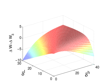
Figure 3: The work difference ($\Delta W-\Delta W_{\delta}$) as a function of $\delta^{h}$ and $\delta^{l}$. The parameters chosen are $p_{0}^{l}=0.5$, $p_{0}^{h}=0.3$, and $KT_{h}=5$. The work difference, $\delta^{x},(x=l,h)$ and $KT_{h}$ were rescaled in units of $KT_{l}=1$ in this plot.

Now, we turn to study the efficiency of this quantum heat engine. It is defined as the ratio of the work done to the heat absorbed in the cycle,

$$\eta=\frac{\Delta W}{\Delta Q}.$$ (17)

By the first law of thermodynamics, we have

$$\eta=1-\frac{\Delta Q_{2}+\Delta Q_{3}}{\Delta Q_{1}+\Delta Q_{4}},$$ (18)

where $\Delta Q_{i}(i=1,2,3,4)$ denote the heat exchange between the working medium and reservoirs on the branch $i$. By the same procedure presented above, one obtains

$$\Delta Q_{1}+\Delta Q_{4} = (p_{0}^{l}-p_{0}^{h})(\Delta^{h}+\delta^{h})$$

$$+ \delta^{h}\cdot f(p_{0}^{x},T_{x},\delta^{x})|_{x=l,h},$$

$$\Delta Q_{2}+\Delta Q_{3} = (p^{l}_{0}-p^{h}_{0})(\Delta^{l}+\delta^{l})$$ (19)

$$+ \delta^{l}\cdot f(p_{0}^{x},T_{x},\delta^{x})|_{x=l,h}.$$

Then the efficiency of the quantum heat engine reads,

$$\eta=1-\frac{(p^{l}_{0}-p^{h}_{0})(\Delta^{l}+\delta^{l})+\delta^{l}\cdot f(p_{0}^{x},T_{x},\delta^{x})|_{x=l,h}}{(p^{l}_{0}-p^{h}_{0})(\Delta^{h}+\delta^{h})+\delta^{h}\cdot f(p_{0}^{x},T_{x},\delta^{x})|_{x=l,h}}.$$

In the high-temperature limit $\frac{\delta^{h}}{KT_{h}}\ll 1,\frac{\delta^{l}}{KT_{l}}\ll 1,$ $\eta$ reduces to

$$\eta=1-\frac{\Delta^{l}+\delta^{l}}{\Delta^{h}+\delta^{h}},$$ (21)

returning back to the efficiency of the two-level quantum heat engine. This observation holds in the low-temperature, as the net work does. Similarly, for $p_{0}^{l}=p_{0}^{h}$, the efficiency becomes $\eta=1-\delta^{l}/\delta^{h}.$ Note that in the limit $\delta^{l}=\delta^{h}$, the net work $\Delta W$ returns back to the result of the two-level quantum heat engine, but the efficiency does not. This is due to the difference in heat exchange of the two engines.

In conclusion, a new quantum heat engine has been introduced in this paper. As its working medium, the quantum system has a discrete level and a continuum. This makes the engine different from the two-level quantum heat engine. The quantum heat engine consists of two adiabatic processes and two isothermal processes. It can extract work like a two-level quantum heat engine in the high-temperature and low-temperature limits, whereas it works in a different way at temperatures between the two. Since the previous studies on quantum heat engine were focused on various working mediums only with discrete energy levels, the study presented here can better the understanding of quantum heat engine, and might provides us a new way to study the unsolved problems of emergence of classicality.

This work was supported by EYTP of M.O.E, NSF of China (10305002 and 60578014).

References

• (1) M. O. Scully, M. S. Zubairy, G. S. Agarwal, H. Walther, Science 299, 862(2003).
• (2) T. D. Kieu, Eur. Phys. J. D 39, 115(2006).
• (3) T. D. Kieu, Phys. Rev. Lett. 93, 140403(2004).
• (4) H. T. Quan, P. Zhang, and C. P. Sun, Phys. Rev. E 72, 056110(2005).
• (5) H. T. Quan, P. Zhang, and C. P. Sun, e-print: quant-ph/0508008.
• (6) H. Scovil and E. Schulz-Dubois, Phys. Rev. Lett. 2, 262(1959).
• (7) S. Lloyd, Phys. Rev. A 56, 3374(1997).
• (8) R. Kosloff, E. Geva, and J. Gordon, J. Appl. Phys. 87, 8093(2000).
• (9) M. O. Scully, Phys. Rev. Lett. 87, 220601(2001).
• (10) M. O. Scully, Phys. Rev. Lett. 88, 050602(2002).
• (11) T. Opatrny, M. O. Scully, Fortschr. Phys. 50, 657(2002).
• (12) Y. V. Rostovtsev, A. B. Matsko, N. Nayako, M. S. Zubairy, and M. O. Scully, Phys. Rev. A 67, 053811(2003).
• (13) T. Feldmann and R. Kosloft, Phys. Rev. E 61, 4774(2000).
• (14) T. Feldmann, E. Geva, R. Kosloff, and P. Salamon, Am. J. Phys. 64, 485(1996).
• (15) C. M. Bender, D. C. Brody, and B. K. Meister, e-print: quant-ph/0101015v2.
• (16) L. D. Noordam, H. Stapelfeldt, D. I. Duncan, and T. F Gallagher, Phys. Rev. Lett. 68, 1496(1992).
• (17) E. Geva and R. Kossloff, J. Chem. Phys. 96, 3054(1992).