Can Bohmian trajectories account for quantum recurrences having classical periodicities?

Abstract

Quantum systems in specific regimes display recurrences at the period of the periodic orbits of the corresponding classical system. We investigate the excited hydrogen atom in a magnetic field – a prototypical system of ’quantum chaos’ – from the point of view of the de Broglie Bohm (BB) interpretation of quantum mechanics. The trajectories predicted by BB theory are computed and contrasted with the time evolution of the wavefunction, which shows pronounced features at times matching the period of closed orbits of the classical hydrogen in a magnetic field problem. Individual BB trajectories do not possess these periodicities and cannot account for the quantum recurrences. These recurrences can however be explained by BB theory by considering the ensemble of trajectories compatible with an initial statistical distribution, although none of the trajectories of the ensemble are periodic, rendering unclear the dynamical origin of the classical periodicities.

I Introduction

The manifestation of classical orbits has been found in a host of quantum systems, displaying features such as scars of wavefunctions along periodic orbits of the corresponding classical system or time recurrences appearing at the periods of classical closed orbits brack badhuri . These features have been observed experimentally in systems such as mesoscopic devices or atoms in external fields. From within a pure Schrödinger based approach, these phenomena may appear as coming out of the blue. They are however well understood by performing asymptotic $\hbar$ expansions. In particular it is straightforward to show (eg, grosche ) that the evolution operator obtained from the path integral expression becomes to first order in $\hbar$

$$\left\langle x_{2},t_{2}\right|e^{-iH(t_{2}-t_{1})/\hbar}\left|x_{1},t_{1}\right\rangle=\left(2i\pi\hbar\right)^{-D/2}\sum_{k}\left|\det\frac{\partial^{2}R_{k}}{\partial x_{2}\partial x_{1}}\right|^{1/2}\exp\frac{i}{\hbar}\left[R_{k}(x_{2},x_{1};t_{2}-t_{1})-\phi_{k}\right]+O(\hbar).$$ (1)

We have assumed for simplicity a time-independent Hamiltonian $H$ in $D$ dimensional configuration space. The sum runs on the classical paths $k$ connecting $x_{1}$ and $x_{2}$ and $R_{k}$ is the classical action along the trajectory $k;$ it satisfies the Hamilton-Jacobi equation of classical mechanics goldstein

$$\frac{\partial R(x,t)}{\partial t}+\frac{(\triangledown R(x,t))^{2}}{2m}+V(x)=0.$$ (2)

The determinant is linked to the classical density and $\phi_{k}$ is an additional phase that keeps track of the points where the classical amplitude is singular. The physical meaning of Eq. (1) is simple: when $\hbar/R$ is small (a situation to be termed here ’semiclassical regime’) propagation in configuration space takes place only along the classical paths, the sum reminding us that the wave takes all the paths simultaneously with a given weight – the classical amplitude.

An alternative interpretation of quantum phenomena hinges on the existence of point-like particles following a well-defined space-time trajectory – a quantum trajectory. The de Broglie Bohm (BB) theory is by far the best-known and most developed of hidden-variables theories, and BB trajectories have been computed for a wide range of quantum systems (see holland93 and Refs therein as well as more recent work e.g. alcantara98 ; nogami00 ; wisniacki03 ; matz05 . One of the main motivations behind the BB theory is to bridge the gap between classical and quantum mechanics. Indeed the interpretation of quantum phenomena by way of a statistical distribution of particles moving along well-defined quantum trajectories appears as an attractive manner of understanding how classical mechanics can emerge from quantum phenomena.

The main concern of this work is to analyze the role of quantum trajectories as predicted by the de Broglie-Bohm interpretation in quantum systems displaying the fingerprints of classical trajectories. In such systems, the wavefunction is carried by classical trajectories, and it is therefore of interest to compare and contrast classical and quantum trajectories. This will be done for a well known prototypical system, an excited hydrogen atom in a magnetic field friedrich wintgen . This system has been heavily investigated, both theoretically and experimentally, in the past 20 years and the success of its semiclassical analysis has converted this sytem into a paradigm of ”quantum chaos” . We will briefly present the main characteristics of this system in Sec. 2. We will then summarize the main properties of BB trajectories and their expected behaviour in the semiclassical regime. Specific quantum trajectories for the hydrogen atom in a magnetic field will be computed in Sec 4. We will see that observable quantum recurrences are ruled by the periodicity of the periodic orbits of the corresponding classical system; the role of the quantum trajectories in accounting for the recurrences will be discussed in Sec 5.

II The hydrogen atom in a magnetic field

The Hamiltonian describing the hydrogen atom in a magnetic field is given by (eg the review paper friedrich wintgen )

$$H=\frac{p^{2}}{2m}+\left(\frac{qBL_{z}}{2mc}-\frac{q^{2}}{r}+\frac{(x^{2}+y^{2})q^{2}B^{2}}{8mc^{2}}\right),$$ (3)

where $B$ is the strength of the magnetic field oriented in the $z$ direction, $\ m$ the mass of the electron, and $r$ the distance of the electron relative to the nucleus. The spherical symmetry of the Coulomb field is broken by the magnetic field, leaving an axial symmetry (invariance around the $z$ axis). We will take $L_{z}=0$ in what follows and we will assume $B$ is sufficiently strong so that perturbation theory is not necessarily valid. It can be shown that $H$ possesses a scaling property, from which it follows that the classical dynamics does not depend independently on the values of the energy $E$ and of the intensity $B$ of the field but on the ratio $\epsilon=EB^{-2/3}$ known as the scaled energy. For $\epsilon\rightarrow-\infty$ the dynamics is near-integrable whereas phase space is fully chaotic for $\epsilon\gtrsim-0.1$ and of mixed nature for $-0.8\gtrsim\epsilon\gtrsim-0.1$.

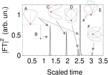
Figure 1: Recurrence spectrum of the hydrogen atom in a magnetic field obtained from quantum computations (Fourier transform of the computed photoabsoption spectrum excited from the ground state with the laser polarized along the field axis). The excitation energy spans the interval $77<n<155$ and the magnetic field varies accordingly so that the scaled energy stays fixed at $\epsilon=-0.3$, thereby obtaining a scaled spectrum. The diagrams show the shape of the orbits closed at the nucleus of the corresponding (scaled) classical problem in the $(\varrho,z)$ plane ($B$ is along the vertical $z$ axis). The arrows indicate the orbit whose period matches the time of a given peak in the recurrence spectrum. Note that more than one orbit can contribute to a given peak, and that the repetitions of an orbit contribute to peaks appearing at multiple integer times of the fundamental period (eg, dotted arrow for the orbit A).

The Schrödinger equation, obtained from the standard quantization of $H$, is simplified by eliminating the trivial azimuthal angle. We are left with a nonseparable 2 dimensional ($\varrho,z$) problem which does not admit analytical solutions; $\varrho,z$ are the rectangular (cylindrical) coordinates in the axial plane. Obtaining the bound energies $E_{n}$ and the eigenfunctions $\psi_{E_{n}}(\varrho,z)$ for highly excited states therefore involves numerical computations with large basis sizes. We will employ atomic units, the energies of the electron being labeled by $E_{n}=-1/2n^{2}$ (where $n$ is of course not an integer). For small $\epsilon$ the energy eigenvalues follow the well known pattern given by perturbation theory (Zeeman effect) but as $\epsilon$ increases the spectrum becomes very complex, as the spherical $n/L$ degeneracy of the free-field atom is totally broken and thousands of energy levels appear. The interpretation of individual levels becomes meaningless, but it was gradually realized that well-resolved peaks are visible by taking a Fourier transform of the photoabsorption spectrum (obtaining what is called a recurrence spectrum). These peaks, related to the large scale fluctuations of the spectrum, appear at times corresponding to periods of classical orbits closed at the nucleus.

A typical computed recurrence spectrum involving photoabsorption from the ground state of the hydrogen atom is given in Fig. 1. Sharp peaks are visible. Above each peak, we have drawn the shape of the classical orbit whose period matches the recurrence time of the peak. This plot arises from quantum calculations, but recurrence spectra have been experimentally observed in hydrogen mainprl as well as other species of one electron (’Rydberg’) atoms delande94 and molecules matz gauyacq in external fields . Purely semiclassical calculations have also been undertaken, reaching an excellent agreement with experimental observations and exact quantum calculations. The semiclassical formalism, known as ’Closed orbit theory’ delos88 , starts from the semiclassical propagator (1) and explains the recurrences observed with classical periodicity by the propagation of the laser excited electron waves along the classical trajectories that start and end at the nucleus: every such orbit produces a peak whose height depends on the classical amplitude of the orbit. If several orbits have the same or nearly the same period (as happens in Fig 1) the height of the peak depends on the interference between the orbits, and the phases $\phi_{k}$ of Eq. (1) play a crucial role.

III De Broglie-Bohm trajectories

The de Broglie-Bohm interpretation of quantum mechanics has become increasingly popular in the last decade and excellent accounts of the theory are available holland93 ; bohm hiley . The main dynamical equations arise from the polar decomposition of the wavefunction in configuration space. Put

$$\psi(\mathbf{r},t)=\rho(\mathbf{r},t)\exp(i\sigma(\mathbf{r},t)/\hbar)$$ (4)

where $\rho$ and $\sigma$ are real functions. The Schrödinger equation becomes equivalent to the coupled equations

$$\frac{\partial\sigma}{\partial t}+\frac{(\triangledown\sigma)^{2}}{2m}+V-\frac{\hbar^{2}}{2m}\frac{\triangledown^{2}\rho}{2\rho} =0$$ (5)

$$\frac{\partial\rho^{2}}{\partial t}+\triangledown(\rho^{2}\triangledown\sigma/m) =0.$$ (6)

$\rho^{2}$ gives the statistical distribution of the particle (here the electron) whereas the trajectory is obtained by integrating the equation of motion

$$\frac{d\mathbf{r}}{dt}=\frac{\mathbf{\triangledown}\sigma(\mathbf{r},t)}{m}$$ (7)

where the initial position of the electron $\mathbf{r}(t=0)$ lies within the initial distribution $\rho(t=0).$ $V$ is the external potential due to the Coulomb and magnetic fields (term between $(...)$ in Eq. (3)) whereas the last term in Eq. (5) acts as a state-dependent ’quantum’ potential.

Despite the formal similarity between Eq. (5) and the classical Hamilton-Jacobi Eq. (2), it is well established that generic quantum trajectories are highly nonclassical holland93 ; appleby . This is still true in the semiclassical regime: the reason is that the nonrelativistic BB theory is grounded on a hydrodynamic framework whereby the local probability density current

$$\mathbf{j}(\mathbf{r},t)=\frac{\hbar}{2mi}\psi^{\ast}(\mathbf{r},t)\overleftrightarrow{\nabla}\psi(\mathbf{r},t)$$ (8)

is linked to the velocity of the particle (7) by

$$\mathbf{j}(\mathbf{r},t)=\rho^{2}(\mathbf{r},t)\mathbf{v}(\mathbf{r},t).$$ (9)

Quantum trajectories are thus tangent to the local flow, as required since two space-time points must be linked by a single trajectory. In the semiclassical approximation however the classical trajectories do not in general follow the flow – rather the flow results from the interfering average of different bits of the wavefunction, each carried by a classical trajectory. Indeed if we assume a wavefunction initially ($t=0$) localized at $\mathbf{r}_{0}$, at later times we have in the semiclassical approximation

$$\psi(\mathbf{r},t)=\sum_{k}A_{k}(\mathbf{r},\mathbf{r}_{0},t)\exp i(R_{k}(\mathbf{r},\mathbf{r}_{0},t)-\phi_{k}),$$ (10)

where $A_{k}$ includes the prefactor given in Eq. (1) and quantities relative to the initial wavefunction. By plugging in Eq. (10) into the expression for the probability density amplitude (8) and comparing with Eq. (9), it is immediate to see that if only a single classical trajectory contributes to the sum (10), we have $\mathbf{j}=\left|A\right|^{2}\triangledown R/m$ and the quantum trajectory approaches the classical one. This is a very restrictive condition: even in conservative one dimensional systems a wavepacket will be carried by several classical trajectories, each having a slightly different energy. The resulting interferences will prevent the BB trajectories to follow the classical ones, as examined in a previous work for radial Rydberg wavepackets matz05 In the general multidimensional case several (quite often an infinity of) trajectories can be launched classically at a given energy from a given $\mathbf{r}_{0}$, and an initial wavepacket will contain a high number of energy eigenstates (depending on the form of the initial wavefunction). $\mathbf{j}$ then contains a double sum involving correlations (in the form of interference terms) between all these classical orbits (see Sec 6.4 of holland93 where an analogue simple example is worked out). Hence, quantum trajectories are not expected to converge toward classical trajectories even in the regime where $\hbar$ becomes negligibly small relative to the classical action (or analogue quantities having dimensions of an action). It is therefore interesting to examine how the de Broglie-Bohm theory accounts for quantum phenomena in which the manifestations of the classical dynamics is apparent, such as the phenomena portrayed in Fig. 1 for the hydrogen atom in a magnetic field.

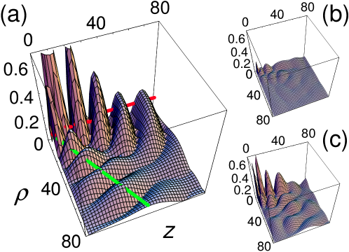
Figure 2: The wavefunction $|\psi(\varrho,z,t)|$ in the region near the nucleus (restricted to the fundamental quadrant, coordinates in atomic units). (a) The initial wavefunction (a radial Gaussian centered at $r_{0}=10$ and an angular distribution in the form of a double bump with maxima at $\theta_{B}$ and $\theta_{C}$) is shown shortly after $t=0$, when the wavepacket starts to propagate. $|\psi|$ is given in units of the highest value of this quantity appearing in the graph. We have also represented 2 trajectories having the same initial position $\mathbf{r}(t=0)=(10,\theta_{C})$: the classical trajectory (green line leaving the nucleus region with a straight angle $\theta_{C}$) and the BB quantum trajectory (red line, which drifted by the main probability flow immediately turns left toward the $z$ axis). (b) The wavefunction near the nucleus at $t=8.9$ ps, when most of the wavepacket has left this region. The vertical scale is the same as in (a). (c) Same as (b) at $t=16.4$ ps when part of the wavepacket returns to the nucleus region, giving rise to the first peak in the autocorrelation function (see Fig. 3).

We will examine some quantum trajectories obtained from the time evolution of an initially chosen wavefunction. In this work we will only be interested in the specific case of recurrences; a full account detailing the global properties of the quantum trajectories for the H atom in a magnetic field problem, in particular as a function of the classical dynamical regime, will be given elsewhere matz-prep . To compute quantum trajectories, we numerically integrate Eq. (7) in the axial $(\varrho,z)$ plane. This is computationally very demanding. First, an initial wavefuntion localized in configuration space results from an expansion of several hundred energy eigenstates $\psi_{E_{k}}(\mathbf{r})$. Second, each of these eigenstates contains several hundred thousand components on the numerical basis, obtained from the diagonalization of very large (but sparse) Hamiltonian matrices friedrich wintgen ; delande94 . Third the integration of Eq. (7), where $\mathbf{\triangledown}\sigma$ is obtained from the logarithmic derivatives of the wavefunction, calls for very small steps when approaching the nodes of the wavefunction. The complexity of the nodal pattern depends on different parameters matz-prep , but the number of nodes increases at least quadratically with the excitation energy. The compromise made was to work with moderately excited states and an initial state that is only approximately localized : in the expansion

$$\psi(\mathbf{r},t=0)=\sum_{k}\alpha_{k}(\mathbf{r}_{0})\psi_{E_{k}}(\mathbf{r})\simeq ce^{-(\mathbf{r}-\mathbf{r}_{0})^{2}/2\Delta r}$$ (11)

the sum over $k$ is restricted so that the Gaussian on the right handside is only approached. Note that besides the axial symmetry, the Hamiltonian (3) possesses a definite symmetry by reflection on both the $z$ and $\varrho$ axis: it is therefore sufficient to consider the upper right ’fundamental’ quadrant ($\varrho$ and $z$ both positive; in polar coordinates $\theta$ refers to the angle with the $z$ axis and varies from 0 to $\pi/2$).

Figure 3: Time variation of the autocorrelation function $|C(t)|^{2}$ (a), the local probability density $|\psi(r^{\prime},\theta_{C},t)|^{4}$ (b) $\left|\psi(r^{\prime},\theta_{B},t)\right|^{4}$ (c), for the initial wavefunction described in the text ($r^{\prime}=60$ au). The time is given in units of the cyclotron period $T_{c}=11.8$ ps and the vertical scale is normalized to the highest value appearing in the graph (for the autocorrrelation function (a), this means that the recurrences account for about $\sqrt{0.14}\simeq 37$% of the initial probability). The letter on a peak refers to the orbit whose period matches the time of the peak maximum (the shape of the relevant orbit is given in Fig. 1).

IV Results

We take an initial state of the form (11) localized near the nucleus with a radial Gaussian peaking at $r_{0}=10$ au and an angular distribution in the form of double bump with maxima at $\theta_{B}=0$ and $\theta_{C}=1.1$ (see Fig. 2). The initial angles are chosen (and therefore labeled) so that they correspond to the angles of the outgoing classical orbits B and C drawn in Fig. 1. The value of the magnetic field is fixed at $B=3$ T and the mean energy of the wavepacket corresponds to $n=55$ (yielding a mean scaled energy of $\epsilon=-0.3$). About 60 states are included in the sum (11), with $n$ in the range 53 to 58 (therefore $\epsilon$ is not strictly fixed like in the case portrayed in Fig. 1). As $t$ increases the wavepacket propagates according to

$$\psi(\mathbf{r},t)=\sum_{k}e^{-iE_{k}t}\psi_{E_{k}}(\mathbf{r})\left\langle\psi_{E_{k}}\right|\left.\psi(t=0)\right\rangle$$ (12)

and reaches regions several thousand of atomic units away from the nucleus. However part of the wavepacket returns to the nucleus: this is readily visible on the autocorrelation function

$$C(t)=\left\langle\psi(t=0)\right|\left.\psi(t)\right\rangle=\sum_{k}\left|\alpha_{k}\right|^{2}e^{-iE_{k}t}$$ (13)

or by simply monitoring the probability density $\left|\psi(r_{0},\theta,t)\right|^{2}.$ Such quantities are plotted on Fig. 3. (a) shows $\left|C(t)\right|$, (b) gives $\left|\psi(r^{\prime},\theta_{C},t)\right|$ and (c) $\left|\psi(r^{\prime},\theta_{B},t)\right|$ where $r^{\prime}\simeq 60$ au is chosen sufficiently far from the nucleus so that the wavepackets converging toward the nucleus from different directions are sufficiently well spatially separated.

The important feature seen in Fig. 3 concerns the presence of isolated peaks. These peaks correspond to recurrences of the wavepacket. These recurrences appear at times correlating with the periods of the closed classical orbits B and C shown in Fig. 1 (the periods are found by numerically integrating the classical equations of motion along the chosen orbit, from which it is found that C has a classical period of 16.3 ps, and B a period of 25.4 ps) .

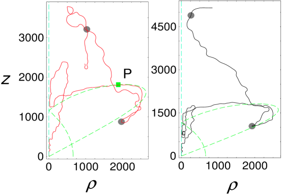
Figure 4: Quantum trajectories (solid lines) in the $(\varrho,z)$ plane, as determined by BB theory when the initial wavefunction is localized near the nucleus ($r_{0}=10$, two bumps at $\theta_{C}$ and $\theta_{B}$). Left panel: initial position of the trajectory at $\mathbf{r}(t=0)=(10,\theta_{C})$, right panel initial position at $\mathbf{r}(t=0)=(10,\theta_{B})$. The dotted lines show the classical trajectories B and C of Fig. 1, leaving the nucleus region with respective angles $\theta_{B}$ and $\theta_{C}$, in the fundamental quadrant (B ([blue dashed] turns back at $z=6000$ a.u., outside the range of the plots; in the fundamental quadrant, C [green-dashed] bounces on the $z$ axis changing branches and is reflected backward by the $\varrho$ axis [compare with the overall shape of the orbit shown in Fig. 1]). The grey dots correspond to the position of the electron along the BB trajectory at times corresponding to the high peaks in the autocorrelation function (Fig. 3a), i.e. the period and twice the period of the classical trajectory C. The square on the left panel locates the point P (see Fig. 6)

The quantum trajectories with initial positions at the maxima of the bumps $\mathbf{r}(t=0)=(10,\theta_{C})$ and $\mathbf{r}(t=0)=(10,\theta_{B})$ (BB_C and BB_B) are shown in Fig. 4 (see also Fig. 2 for a closeup of BB_C near the nucleus). The shape of both trajectories is at first similar, although BB_B spends more time near the $z$ axis. It is readily apparent that neither BB_C nor BB_B come back to the region near the nucleus at times compatible to account for the recurrence peaks seen in Fig. 3 (the positions of the Bohmian particle at the time of the first two peaks seen in the autocorrelation function is shown in Fig 4).

Fig. 5 shows other typical examples of quantum trajectories. The left panel shows quantum trajectories for the same initial distribution as in Fig. 4 but different initial positions. The right panel shows the quantum trajectories with the same initial conditions as in Fig. 4 but for a slightly different initial wavefunction: in the sum defining the initial wavefunction in Eq. (11), we have left out the first and the last terms. If we would have plotted the new initial wavefunction as in Fig. 2, the difference would not be visible to the eye; neither would the time dependent functions shown in Fig. 3(a) and (b) be different on the scale of the plots (Fig. 3(c) would be barely different). However the BB trajectories plotted in Fig. 5 (right) are markedly different from their counterpart of Fig. 4.

V Discussion and conclusion

We have seen for a specific initial wavefunction the presence of quantum recurrences appearing at times matching the period of classical orbits closed at the nucleus. As mentioned above, this behaviour has been experimentally observed in the recurrence spectra of hydrogen and other Rydberg atoms in a magnetic field friedrich wintgen ; mainprl ; delande94 . The dynamical interpretation of such experiments and of the results shown in Fig. 3 relies on semiclassical arguments: most of the initial wavefunction was chosen to sit near the nucleus in regions overlapping with the classical trajectories B and C. Since according to Eq. (10) the wavefunction is carried by the classical trajectories, a recurrence seen at time $T$ corresponds to the part of the wavepacket that returns to the nucleus along the classical trajectory with period $T$. According to these semiclassical arguments, the wave simultaneously travels along the available paths – this is an instance of a sum over paths, not an application of the Erhenfest theorem. If this sum over paths picture makes sense, then by monitoring the probability amplitude at some space point along a chosen orbit, one should detect the passage of the wavepacket at times compatible with classical motion. This is indeed the case, as shown in the example given in Fig. 6 for the point P chosen on the closed orbit C. Classically, the travel time from the initial position $\mathbf{r}(t=0)=(10,\theta_{C})$ to P is about $0.43$ $T_{c}$; the classical particle continues to travel along C, reflects on the $\varrho$ axis and travels backward, reaching P about $0.48$ $T_{c}$ later. The first 2 recurrence peaks seen in Fig. 6 agree with these classical times. The two last peaks on the right appear at times reflecting the shift of the first 2 peaks by one classical period of the orbit C, about $1.4$ $T_{c}$.

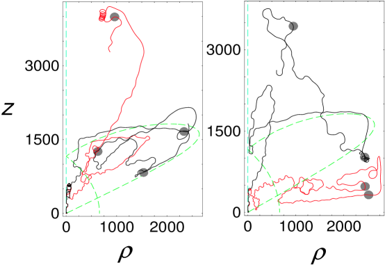
Figure 5: Quantum trajectories. Left panel: same as Fig. 4 but with the following initial conditions: $\mathbf{r}(t=0)=(5,\theta_{C})$ (red line) and $\mathbf{r}(t=0)=(9,0.25)$ (black line). Right panel: same as Fig. 4 [$\mathbf{r}(t=0)=(10,\theta_{C})$ (red) and $\mathbf{r}(t=0)=(10,\theta_{B})$ (black)] but when the initial wavefunction is slightly different (see text); although the wavefunction dynamics is globally almost identical in both cases, the BB trajectories are different.

As mentioned in Sec. 3, the de Broglie-Bohm trajectories are directly related to the density current. As can partially be inferred from Fig. 2, the density current is at first higher near the $z$ axis: this is why BB_C quickly turns left and escapes along this axis. Now we have remarked that only a fraction of the initial wavefunction actually returns to the nucleus to produce the observed recurrences. It is therefore quite improbable that a particle with initial position at a probability maximum leaving the nucleus region by following the main current will return to the nucleus to account for the observed recurrences. From this perspective the fact that the BB trajectories initially near the maximum of the probability distribution are very far from the nucleus when the recurrences are produced, as testified by the dots in Fig. 4, is not surprising. This appears to be a generic property of BB trajectories for systems in the semiclassical regime, as discussed in Sec. 3. Of course, needless to mention that this point has nothing to do regarding the capacity of BB theory to account for these recurrences. This simply entails that the partial revival of the wavefunction seen e.g. in Fig 2(c), that translates as a peak in the autocorrelation function, should be attributed to a Bohmian particle that occupied at $t=0$ a point in configuration space away from the probability maximum of the distribution. The precise initial position of such a particle will depend on the system specifics (current density and initial state). In the present case, although the highest values of the initial probability distribution are found by far near the nucleus, the probability outside this zone is not zero (although it is several orders of magnitude below the value near the nucleus). Hence the initial positions of the Bohmian particle accounting for the recurrences can be found inside or outside the nucleus region (for instance the BB trajectory arriving exactly at $(r_{0},\theta_{C})$ at the period of trajectory C was at $t=0$ near $\varrho=700$, $z=128$ au, where the initial probability is 4 orders of magnitude less than near the nucleus). We therefore see that on the statistical level the recurrences can be explained by taking into account the ensemble of different initial positions, scattered throughout all of configuration space, that lead the particle to the nucleus region at times corresponding to the observed recurrences. As another illustration take the recurrences at P seen in Fig. 6: the BB trajectory BB_C (having its initial position on the bump corresponding to the initial position of the orbit C) also goes through P (Fig. 3), reaching P at $t=0.97$ $T_{c}$. Therefore this quantum trajectory can account for the second peak seen in Fig. 6, but not for the first nor the last two peaks. BB trajectories going through P to account for these other peaks do exist (they all have different initial conditions). However although according to the propagator (1) these classical-time recurrences are due to the propagation of a part of the wavefunction on a classical periodic orbit, there is no such dynamical explanation in terms of the motion of a Bohmian particle on a given trajectory.

It is also worth noticing that is not unusual for the BB trajectories to follow some segments of classical trajectories. For example in Fig. 4 BB_C and BB_B follow at short times the B orbit parallel to the $z$ axis, and then tend to organize around C for some time (both BB orbits go from the $z$ axis, through P, and turn with C). Indeed when a classical trajectory travels along the current density gradient, a nearby BB trajectory will present the same motion. But as a general rule classical trajectories cross and the net current ruling the BB motion arises from the resulting interference (the simplest example being the one-dimensional infinite well, where the classical to and from motion results in an interference leading to a static net current and hence no BB motion, e.g. Sec. 6.5 of holland93 ).

The detailed motion of the Bohmian particle also depends on the dynamics of the nodes, which may either trap the particle for a long time or violently separate two nearby BB trajectories (examples will be given elsewhere matz-prep ). The result is that BB trajectories are in general considerably more complex than the classical ones, as recently put in evidence in the case of stadium billiards wisniacki03 . This is why as seen in Fig. 5 a slight change in the initial wavefunction which barely affects the subsequent time-evolution of observable (and statistical) quantum quantities may give rise to very different BB trajectories. Indeed the quantum potential is very sensitive to locally fine details of the evolving wavefunction. Therefore two slightly different wavefunctions may give rise, in terms of the Bohmian particle, to different dynamics (compare the red curves in the left panel of Fig. 4 and the right panel of Fig. 5, which have the same initial position). On the other hand, the semiclassical arguments are the same for both initial wavefunctions whose large-scale structures depend on the underlying classical dynamics identical in both cases, the relative weight of the interfering trajectories being different.

Figure 6: $\left|\psi(\varrho_{P},z_{P},t)\right|^{4}$ is given as a function of the cyclotron period $T_{c}$; P is a point chosen on the closed classical trajectory C (the position of P is shown in Fig. 4).

To summarize, we have investigated wavepacket dynamics of the hydrogen atom in a magnetic field when the wavepacket is initially localized near the nucleus. This quantum system displays the fingerprints of classical trajectories in the form of recurrences appearing at times matching the periods of the closed orbits of the classical system. These features are well understood within the semiclassical approximation to the path integral propagator, grounded on the properties of the classical trajectories. Quantum trajectories computed according to the de Broglie Bohm theory do not display such periodicities: individual trajectories are highly nonclassical and cannot explain the observed recurrences. Their dynamics is governed by the local current density which for highly excited systems is extremely complex. The recurrences are nevertheless accounted for statistically by the arrival at the recurrence times of particles whose initial positions were preferentially away from the maximum of the initial distribution. This statistical explanation may seem to lack a dynamical determination concerning the particle: the manifestation of the classical motion apparent in the large scale structures of the wave propagation, inducing the partial periodicity of the quantum system, has no counterpart in the motion of the Bohmian particle, guided by the local details of de Broglie’s ’pilot-wave’ (along the probability current density). Possible consequences regarding the emergence of classical trajectories from quantum mechanics in a de Broglie-Bohm framework will be examined in a future work.

References

- (1) M Brack and R. K. Bhaduri, Semiclassical Physics, Addison-Wesley, Reading (USA), 1997.
- (2) C. Grosche and F. Steiner, Handbook of Feynman Path Integrals, Springer Tracts in Modern Physics 145 (1998), in particular Ch. 5.
- (3) H. Goldstein, Classical Mechanics, Addison-Wesley, Reading (USA), 1980.
- (4) P.R. Holland, The Quantum Theory of Motion, Cambridge Univ. Press, Cambridge (1993).
- (5) O. F. de Alcantara Bonfim, J. Florencio and F. C. S Barreto, Phys. Rev. E 58, R2693 (1998).
- (6) Y. Nogami, F. M. Toyama and W. van Dijk, Phys. Lett. A 270, 279 (2000).
- (7) D. A. Wisniacki, F. Borondo and R. M. Benito, Europhys. Lett. 64, 441 (2003).
- (8) A. Matzkin, Phys. Lett. A 345, 31 (2005).
- (9) H. Friedrich and D. Wintgen, Phys. Rep. 183, 37 (1989).
- (10) A. Holle, J. Main, G. Wiebusch, H. Rottke, and K. H. Welge, Phys. Rev. Lett. 61, 161 (1988).
- (11) D. Delande, K.T. Taylor, M.H. Halley, T. Van der Veldt, W. Vassen and W. Hogervorst, J. Phys. B 27, 2771 (1994).
- (12) A. Matkin, M. Raoult and D. Gauyacq, Phys. Rev. A 68, 061401(R) (2003).
- (13) M. L. Du and J. B. Delos, Phys. Rev. A 38, 1896 (1988).
- (14) D. Bohm and B. J. Hiley, The Undivided Universe, Routledge, London, 1993.
- (15) D. M. Appleby, Found. Phys. 29, 1863 (1999).
- (16) A. Matzkin, in preparation.