Quantum simulations under translational symmetry

Abstract

We investigate the power of quantum systems for the simulation of Hamiltonian time evolutions on a cubic lattice under the constraint of translational invariance. Given a set of translationally invariant local Hamiltonians and short range interactions we determine time evolutions which can and those that can not be simulated. Whereas for general spin systems no finite universal set of generating interactions is shown to exist, universality turns out to be generic for quadratic bosonic and fermionic nearest-neighbor interactions when supplemented by all translationally invariant on-site Hamiltonians.

I Introduction

One of the most promising applications of quantum computers is that of being a working horse for physicists who want to determine the time evolution of a theoretically modeled quantum system. On a classical computer this is a daunting task burdened by the notorious exponential growth of the underlying Hilbert space. As pointed out by Feynman Feynman ; Lloyd , quantum systems can, however, be used to efficiently simulate quantum mechanical time evolutions—provided that we have sufficient coherent control on the system. In this direction enormous progress has been made during the last years, in particular in systems of optical lattices opticallattices and ion traps iontraps ; Diego . Moreover, it was realized that quantum simulators Jane are much less demanding than quantum computers and, in fact, pioneering experiments simulating quantum phase transitions in systems of cold atomic gases opticallattices have already turned some of the visions QPTheorie into reality.

One of the fundamental questions in the field of quantum simulations is the following: Given a set of interactions we can engineer with a particular system, which are the Hamiltonians that can be simulated? Concerning gates, i.e., discrete time unitary evolutions, it has been shown in the early days of quantum information theory that almost any two-qubit gate is universal 2universality . Similarly, any fixed entangling two-body interaction was shown to be capable of simulating any other two-body Hamiltonian when supplemented by the set of all local unitaries 2body . The many-body analogue of this problem was solved in manybody and the efficiency of quantum simulations was studied in various contexts (cf. eff ).

All these schemes are based on the addressing of sites, i.e., local control. Imagine now that we have a chain in which we cannot address each particle individually but only apply global single-particle and nearest-neighbor interactions. Can we simulate the evolution of a next-to-nearest neighbor interaction Hamiltonian, or obtain some long-range (e.g., dipole) coupling, or even a three-particle interaction Hamiltonian?

In this article we will concentrate on the case in which the interactions at hand are short range and translationally invariant as it is (approximately) the case in different experimental set-ups, like in the case of atoms in optical lattices or in many other systems that naturally appear in the context of condensed matter and statistical physics. In order to make the problem mathematically tractable and to exploit its symmetries we will consider periodic boundary conditions, even though typically physical systems have open ones. In this sense, our results may not be directly applicable to certain physical situations. In any case, we expect that our work will be a step forward to the establishment of what can and cannot be simulated with certain quantum systems. We will consider three different systems: spins, fermions and bosons. A summary of the results of this work is given in the following section.

II statement of the problem and summary of results

Consider a cubic lattice of $N$ sites with periodic boundary conditions in arbitrary spatial dimension. Assume that we can implement every Hamiltonian from a given set $\mathcal{S}=\{\mathcal{H}_{1},\mathcal{H}_{2},\ldots\}$ of translationally invariant Hamiltonians and in this way achieve every unitary time evolution of the form $e^{i\mathcal{H}_{j}t}$ for arbitrary $t\in\mathbb{R}$. Note that this assumes that both $\pm\mathcal{H}_{j}$ are available. The question we are going to address is, which evolutions can be simulated by concatenating evolutions generated by the elements of $\mathcal{S}$. Our main interest lies in sets which contain all on-site Hamiltonians and specific nearest-neighbor interactions.

The natural language for tackling this problem is the one of Lie algebras FultonHarris ; Cornwell since the set of reachable interactions is given by the Lie algebra $\mathcal{L}$ generated by the set $i\mathcal{S}$. This follows from the Lie -Trotter formulae LieTrotter

$$e^{\alpha L_{k}+\beta L_{l}} = \lim_{n\rightarrow\infty}\left(e^{\alpha L_{k}/n}e^{\beta L_{l}/n}\right)^{n},\quad\alpha,\beta\in\mathbb{R},$$

$$e^{[L_{k},L_{l}]} = \lim_{n\rightarrow\infty}\left(e^{L_{k}/\sqrt{n}}e^{L_{l}/\sqrt{n}}e^{-L_{k}/\sqrt{n}}e^{-L_{l}/\sqrt{n}}\right)^{n},$$

where $L_{k}$ is a representation of the generator $i\mathcal{H}_{k}$. When applying the Lie-Trotter formulae to the elements of $i\mathcal{S}$ we can obtain all commutators and real linear combinations of its elements, i.e., we end up with the Lie algebra generated by $\mathcal{S}$. Conversely, it follows from the Baker-Campbell-Haussdorff formula BCH that all simulatable interactions can be written in this way. We will study the cases of $D$-dimensional ‘spin’ systems ($\mathcal{L}\subset su_{D^{N}}$) as well as quadratic Hamiltonians in fermionic ($\mathcal{L}\subset so_{2N}$) and bosonic ($\mathcal{L}\subset sp_{2N}$) operators. The following gives a simplified summary of the main results. Hamiltonians and interactions are meant to be translationally invariant throughout and it is assumed that interactions along different directions can be implemented independently.

• Fermions: All simulated evolutions have real tunneling/hopping amplitudes. Within this set generic nearest-neighbor interactions are universal for the simulation of any translationally invariant interaction when supplemented with all on-site Hamiltonians. Whereas for cubes with odd edge length the proof of universality requires interactions along all axes and diagonals, the diagonals are not required for even edge length.

• Bosons: All simulated evolutions are point symmetric. Within this set every nearest-neighbor interaction (available along axes and diagonals) is universal for the simulation of any translationally invariant interaction when supplemented with all on-site Hamiltonians.

• Spins: There is no universal set of nearest-neighbor interactions. Moreover, if $f$ is a factor of the edge length $m$ of the cubic lattice then there is no universal set of interactions with interaction range smaller than $f$. In particular, if $m$ is even, not all next-to-nearest neighbor interactions can be simulated from nearest neighbor ones. Sets of Hamiltonians that can be simulated are constructed.

Whereas in the case of quadratic bosonic and fermionic Hamiltonians a rather exhaustive characterization of simulatable time evolutions is possible, a full characterization of simulatable spins systems still remains an open problem.

We will start with introducing some preliminaries on quadratic Hamiltonians in Sec.III. Sec.IV will then treat fermionic and Sec.V bosonic systems. Both start with the one-dimensional case which is then generalized to arbitrary dimensional cubic lattices. Finally spin systems are addressed in Sec.VI.

III Quadratic Hamiltonians

This section will introduce the basic notions and the notation used in Secs. IV,V. The presentation is a collection of tools widely used in the literature on translationally invariant quasi-free fermionic LSM ; Araki ; Bravyi ; Wolf and bosonic Audenaert-Eisert-Werner ; Schuch systems. We consider a system of $N$ fermionic or bosonic modes characterized by a quadratic Hamiltonian

$$\mathcal{H}=\sum_{k,l=1}^{N}A_{kl}a_{k}a_{l}+B_{kl}a_{k}a_{l}^{\dagger}+C_{kl}a_{k}^{\dagger}a_{l}+D_{kl}a_{k}^{\dagger}a_{l}^{\dagger}.$$ (1)

Here, $a_{k}^{\dagger}$ and $a_{k}$ are creation and annihilation operators satisfying the canonical (anti)-commutation relations

$$\mbox{CAR: }\{a_{k},a_{l}\} = 0,\;\;\{a_{k},a_{l}^{\dagger}\}=\delta_{kl}\;\;\mbox{(fermions)},$$ (2)

$$\mbox{CCR: }\left[a_{k},a_{l}\right] = 0,\;\;[a_{k},a_{l}^{\dagger}]=\delta_{kl}\;\;\mbox{(bosons)}.$$ (3)

By defining a vector $\alpha=(a_{1},\ldots,a_{N},a_{1}^{\dagger},\ldots a_{N}^{\dagger})$ and a Hamiltonian matrix

$$\tilde{H}=\left(\begin{array}[]{cc}A&B\\ C&D\\ \end{array}\right)$$ (4)

Eq.(1) can be written in the compact form $\mathcal{H}=\alpha\tilde{H}\alpha^{T}$. The Hermiticity of $\mathcal{H}$ implies the relations

$$B=B^{\dagger},\;C=C^{\dagger}\;,A=D^{\dagger}.$$ (5)

We will identify Hamiltonians which differ by multiples of the identity as they give rise to undistinguishable time evolutions. The commutation relations can then be exploited to symmetrize the Hamiltonian matrix $\tilde{H}$ such that

$$A=\tau A^{T},D=\tau D^{T},B=\tau C^{T},$$ (6)

where $\tau=1$ for bosons and $\tau=-1$ in the case of fermions. Instead of working with $2N$ creation and annihilation operators it is often convenient to introduce $2N$ hermitian operators $c_{k}$ via

$$c_{k}=(a_{k}^{\dagger}+a_{k})/\sqrt{2},\;\;c_{k+N}=i(a_{k}^{\dagger}-a_{k})/\sqrt{2}.$$ (7)

In the case of fermions these are the Majorana operators obeying the anti-commutation relation

$$\{c_{k},c_{l}\}=\delta_{kl}.$$ (8)

For bosons the $c_{k}$ are the position and $c_{k+N}$ momentum operators, and the commutation relations can be expressed in terms of the symplectic matrix $\sigma$ via

$$[c_{k},c_{l}]=i\sigma_{kl},\;\;\sigma=\left(\begin{array}[]{cc}0&\mbox{$1{\bf l}$}\\ -\mbox{$1{\bf l}$}&0\\ \end{array}\right),\;\;\mbox{$1{\bf l}$}\in\mathbb{R}^{N\times N}.$$ (9)

Eq. (1) can now be written in the form

$$\mathcal{H}=\frac{\sqrt{\tau}}{2}\sum_{k,l}H_{kl}c_{k}c_{l},\ \ \ H=\left(\begin{array}[]{cc}X&W\\ \tau W^{T}&Y\\ \end{array}\right).$$ (10)

Exploiting again the commutation relations we can choose the Hamiltonian matrix $H$ real and (anti-) symmetric with $H=\tau H^{T}$. The Hamiltonian matrices of the two representations are related via

$$\tilde{H}=\frac{\sqrt{\tau}}{4}{\small\left(\begin{array}[]{cc}X-Y-i(W+\tau W^{T})&X+Y+i(W-\tau W^{T})\\ X+Y-i(W-\tau W^{T})&X-Y+i(W+\tau W^{T})\\ \end{array}\right)}.\vspace*{3pt}$$

Time-evolution: We are interested in time-evolutions generated by quadratic Hamiltonians of the form in Eq. (1). These are canonical transformations which preserve the (anti-) commutation relations and act (in the Heisenberg picture) linearly on the $c_{k}$’s:

$$e^{i\mathcal{H}t}c_{k}e^{-i\mathcal{H}t}=\sum_{l=1}^{N}T_{lk}c_{l}\;.$$ (11)

In the fermionic case the CAR are preserved iff $T\in O(2N)$ is an element of the orthogonal group in $2N$ dimensions. This group has two components corresponding to elements with determinant $\pm 1$. As time evolution has to be in the part connected to the identity (for $t=0$) we have that $T\in SO(2N)$ is an element of the special orthogonal group. For bosons the preservation of the commutation relations implies that $T$ is a symplectic matrix, i.e. $T\sigma T^{T}=\sigma$. Both groups $SO(2N)$ and $Sp(2N)$ are Lie groups and we can express $T$ in terms of the exponential map acting on the respective Lie algebra, i.e., $T=e^{tL}$. From the infinitesimal version of Eq.(11) we obtain a simple relation between the generator $L$ and the Hamiltonian matrix $H$:

$$L = -H\;\;\,\,\,\mbox{for fermions}$$ (12)

$$L = H\sigma^{T}\;\;\mbox{for bosons}.\vspace*{3pt}$$ (13)

Translational invariant systems: We will throughout consider translationally invariant systems on cubic lattices in $d$ spatial dimensions with periodic boundary conditions. Hence, the indices of the Hamiltonian matrix $H_{kl}$ which correspond to two points on the lattice are $d$-component vectors $k,l\in\mathbb{Z}^{d}_{m}$ where $m$ is the edge length of the cube, i.e., $N=m^{d}$. The translational invariance is expressed by the fact that the matrix elements $G_{kl}$, of the blocks $G\in\{X,Y,W\}$ of $H$ depend only on the relative distance $k-l$. Taking into account the periodic boundary conditions, $k-l$ is understood modulo $m$ in each component. Such matrices are called circulant, and we will denote by $\mathcal{C}_{A}$ and $\mathcal{C}_{S}$ the set of circulant symmetric and antisymmetric matrices, respectively. All circulant matrices can be diagonalized simultaneously by Fourier transformation

$$\hat{G}\equiv\mathcal{F}^{\otimes d}G\mathcal{F}^{\dagger\otimes d} = \mbox{diag}\left[\sum_{k\in\mathbb{Z}^{d}_{m}}G_{k}e^{-\frac{2\pi i}{m}kl}\right]_{l},$$ (14)

$$\mathcal{F}_{pq} = \frac{1}{\sqrt{m}}e^{\frac{2\pi i}{m}pq},\;\;p,q\in\mathbb{Z}_{m},$$ (15)

where $G_{k}\equiv G_{k,0}$ is the entry of the $k$-th off-diagonal of the matrix $G$. It follows from (14) that all circulant matrices mutually commute.

IV Simulations in fermionic systems

In this section we study the set of interactions that can be simulated in a translationally invariant fermionic system starting with quadratic local transformations and nearest neighbor-interactions. Making use of the fact that the blocks $X,Y$ and $W$ in Eq.(10) mutually commute we calculate the commutator $L^{\prime\prime}=[L,L^{\prime}]$ of two generators $L$ and $L^{\prime}$ given by

$$L^{(\prime)}=\left(\begin{array}[]{cc}X^{(\prime)}&W^{(\prime)}\\ -W^{(\prime)T}&Y^{(\prime)}\\ \end{array}\right)$$ (16)

and obtain

$$L^{\prime\prime}={\small\left(\begin{array}[]{cc}X^{\prime\prime}&W^{\prime\prime}\\ -W^{\prime\prime T}&-X^{\prime\prime}\\ \end{array}\right)},\;\begin{array}[]{lcl}X^{\prime\prime}&=&W^{\prime}W^{T}-WW^{\prime T}\\ W^{\prime\prime}&=&W(Y^{\prime}-X^{\prime})\\ &&-W^{\prime}(Y-X)\end{array}$$ (17)

Note that by Eq.(17) every commutator has the symmetry $Y^{\prime\prime}=-X^{\prime\prime}$. Hence, if we start with a set $\mathcal{S}$ of Hamiltonians with corresponding generators $\mathcal{S_{L}}=\{L_{1},L_{2},\ldots\}$, then every element of the generated Lie algebra $\mathcal{L}$ has this form up to linear combinations of elements in $\mathcal{S_{L}}$. On the level of Hamiltonians this symmetry corresponds to real tunneling/hopping coefficients $B_{kl}=-C_{lk}\in\mathbb{R}$ in Eq.(1). We will denote by $\mathcal{R}$ the vector space of all matrices of the form (16) for which $Y=-X$.

Let us now introduce the elements of the set $\mathcal{S_{L}}$ corresponding to all local Hamiltonians and specific nearest-neighbor interactions. Every generator $L$ of a local Hamiltonian is proportional to

$$E=\left(\begin{array}[]{cc}0&\mbox{$1{\bf l}$}\\ -\mbox{$1{\bf l}$}&0\\ \end{array}\right).$$ (18)

For giving an explicit form to the nearest-neighbor interaction, we define a matrix $M^{(v)}$ via

$$M^{(v)}_{kl}=\delta_{l,k+v},$$ (19)

where $v,k,l\in\mathbb{Z}_{m}^{d}$ and the addition is modulo $m$ in each of the components. This leads to the properties

$$M^{(v_{1})}M^{(v_{2})}=M^{(v_{1}+v_{2})},\ \ M^{(0)}=\mbox{$1{\bf l}$}.$$ (20)

Moreover, we define the matrices

$$M^{(v)}_{+} = M^{(v)}+M^{(-v)},\ \ M^{(v)}_{-}=M^{(v)}-M^{(-v)},\ \ \ \$$ (21)

$$H_{X}^{(v)} = {\small\left(\begin{array}[]{cc}M^{(v)}_{-}&0\\ 0&-M^{(v)}_{-}\\ \end{array}\right)},$$ (24)

$$H^{(v)}_{W(\pm)} = {\small\left(\begin{array}[]{cc}0&M^{(v)}_{(\pm)}\\ M^{(v)T}_{(\pm)}&0\\ \end{array}\right)},$$ (27)

where the indices $X$ and $W$ refer to a non-vanishing $X$- and $W$-block respectively. Denoting by $e_{i}\in\mathbb{Z}_{m}^{d}$ the basis vectors $(e_{i})_{j}=\delta_{ij}$, every Hamiltonian matrix corresponding to a nearest-neighbor interaction along $e_{i}$ is of the form

$$H_{0}\equiv\left(\begin{array}[]{cc}X_{0}&W_{0}\\ -W_{0}^{T}&Y_{0}\\ \end{array}\right)=$$ (30)

$$\left(\begin{array}[]{cc}xM^{(e_{i})}_{-}&wM^{(e_{i})}+\tilde{w}M^{(-e_{i})}\\ -(\tilde{w}M^{(e_{i})}+wM^{(-e_{i})})&yM^{(e_{i})}_{-}\\ \end{array}\right),$$ (33)

where $x,y,w,\tilde{w}\in\mathbb{R}$. We will now start studying one-dimensional systems and then generalize to the $d$-dimensional case.

IV.1 Simulations in one-dimensional fermionic systems

In this section we consider quadratic fermionic Hamiltonians with translational symmetry on a ring of $m$ sites. We will give an exhaustive characterization of nearest-neighbor Hamiltonians which are universal for the simulation of all interactions obeying the symmetry $Y=-X$, when supplemented by all on-site Hamiltonians. The results depend on whether $m$ is even or odd.

Theorem 1

Consider a translationally invariant fermionic systems of $m$ sites on a ring with periodic boundary conditions. Starting with all one-particle transformations which are proportional to the matrix $E$ defined in (18) and one nearest-neighbor interaction $H_{0}$ of the form (30) we can simulate the following set of interactions depending on the symmetry properties of $X_{0},Y_{0}$ and $W_{0}$:

1. $m=2n+1$ odd:

   1. $X_{0}=Y_{0},W_{0}\in\mathcal{C}_{S}$: No further interaction can be simulated.

   2. $X_{0}\neq Y_{0}$ or $W_{0}\notin\mathcal{C}_{S}$: The space $\mathcal{R}$ (i.e. $X=-Y$) can be simulated.

2. $m=2n$ even:

   1. $X_{0}=Y_{0},W_{0}\in\mathcal{C}_{S}$: No further interaction can be simulated.

   2. $W_{0}\in\mathcal{C}_{A}$ or $W_{0}=0$: The space spanned by

      $$\mathcal{I}\equiv\{H^{((2k-1)e_{1})}_{X},H^{(2ke_{1})}_{W+},H^{((2k-1)e_{1})}_{W-}\}_{k\in\mathbb{N}}$$

      can be simulated. (For the definition of $H_{X}$ and $H_{W}$ see Eqs. (24), (27) ).

   3. $W_{0}\notin\mathcal{C}_{A},H_{0}\in\mathcal{R}$: The space $\mathcal{R}$ can be simulated.

   4. $W_{0}\notin\mathcal{C}_{A},H_{0}\notin\mathcal{R}$: The space spanned by

      $$\mathcal{J}\equiv\{H^{(ke_{1})}_{X},H^{(2ke_{1})}_{W},H^{((2k-1)e_{1})}_{W}-H^{((2(k-1)-1)e_{1})}_{W}\}_{k\in\mathbb{N}}$$

      can be simulated.

Proof For the proof we will need the relations

$$[H_{X}^{(ke_{1})},E] = 2H_{W-}^{(ke_{1})},$$ (34)

$$\,[E,H_{W}^{(ke_{1})}] = H_{X}^{(ke_{1})},$$ (35)

$$\,[H_{X}^{(ke_{1})},H_{X}^{(le_{1})}] = 0,\ \ \ \ \$$ (36)

$$\,[H_{X}^{(ke_{1})},H_{W}^{(le_{1})}] = 2(H_{W}^{((l+k)e_{1})}-H_{W}^{((l-k)e_{1})}),\quad$$ (37)

$$\,[H_{W}^{(ke_{1})},H_{W}^{(le_{1})}] = H_{X}^{((l-k)e_{1})}.$$ (38)

For $X_{0}=Y_{0},W_{0}\in\mathcal{C}_{S}$, $[H_{0},E]=0$ according to (17) so that we cannot simulate any further interaction (up to multiples of $E$). This proves (1a) and (2a).
If $W_{0}\notin\mathcal{C}_{S}$ or $X_{0}\neq Y_{0}$, we will show in the first step by induction over $k$ that the set $\mathcal{I}$ defined in (2b) can be simulated. For $k=1$, we can get $H_{X}^{(e_{1})}$ and $H_{W-}^{(e_{1})}$ by taking the commutator of $H_{0}$ with the one-particle transformation $E$: If $W_{0}\in\mathcal{C}_{S}$, then $[H_{0},E]\sim H_{W-}^{(e_{1})}$ and $H_{X}^{(e_{1})}$ can be obtained using (35). If $X_{0}=Y_{0}$, then $[H_{0},E]\sim H_{X}^{(e_{1})}$ and we get $H_{W-}^{(e_{1})}$ by (34). If $W_{0}\notin\mathcal{C}_{S}$ and $X_{0}\neq Y_{0}$, then

$$[H_{0},E]/(\tilde{w}_{0}-w)+[[H_{0},E],E]/2(x_{0}-y_{0})\sim H_{W-}^{(e_{1})}$$

and according to (35) we also get $H_{X}^{(e_{1})}$. From (37) we see that we get

$$H_{W+}^{(2e_{1})}=[H_{X}^{(e_{1})},H_{W-}^{(e_{1})}]/2+2E.$$

Now let $k\geq 1$. Using (37) and (35) we get

$$[H_{X}^{(e_{1})},H_{W+}^{(2ke_{1})}]+H_{W-}^{((2k-1)e_{1})}=H_{W-}^{((2(k+1)-1)e_{1})}$$

which implies that we also get $H_{X}^{((2(k+1)-1)e_{1})}$. As

$$[H_{X}^{(e_{1})},H_{W-}^{((2(k+1)-1)e_{1})}]+H_{W+}^{(2e_{1})}=H_{W+}^{(2(k+1)e_{1})},$$

we have shown that we can simulate $\mathcal{I}$. Using the relations (34) - (38), we see that $\mathcal{I}$ is closed under the commutator bracket.
If $m=2n+1$, $\mathcal{I}$ is a basis of all possible interactions of the space $\mathcal{R}$ because of the periodic boundary conditions. To see this, define for an arbitrary $k$ the number $k^{\prime}=k+n+1$. As $2k^{\prime}\mbox{mod}\,m=2k+1$, we see that $H_{X}^{((2k^{\prime}-1)e_{1})}=H_{X}^{(2ke_{1})},H_{W-}^{((2k^{\prime}-1)e_{1})}=H_{W-}^{(2ke_{1})}$ and $H_{W+}^{(2k^{\prime}e_{1})}=H_{W+}^{(2(k+1)e_{1})}$, which proves (1b).
Now let $m=2n$. If $W_{0}\in\mathcal{C}_{A}$ or $W_{0}=0$, then

$$H_{0}=\tilde{H}+w_{0}H_{W}^{(e_{1})},\;\;\;\tilde{H}={\footnotesize\left(\begin{array}[]{cc}x_{0}M_{-}^{(e_{1})}&0\\ 0&y_{0}M_{-}^{(e_{1})}\\ \end{array}\right)}\notin\mathcal{I}.$$

The elements of $\mathcal{I}$ are the only ones that can be simulated as

$$[\tilde{H},H_{W\pm}^{(le_{1})}]=(x_{0}-y_{0})[H_{X}^{(e_{1})},H_{W\pm}^{(le_{1})}]\in\mathcal{I}$$

where $l=2k,2k-1$ respectively and $\tilde{H}$ commutes with $H_{X}^{((2k-1)e_{1})}$. This proves (2b).
If $W_{0}\notin\mathcal{C}_{A}$ and $H_{0}\in\mathcal{R}$, then

$$H_{0}=x_{0}H_{X}^{(e_{1})}-\tilde{w}_{0}H_{W-}^{(e_{1})}+(w_{0}+\tilde{w}_{0})H_{W}^{(e_{1})}$$

so that we can extract $H_{W}^{(e_{1})}$. According to (37)

$$[H_{X}^{((2k-1)e_{1})},H_{W}^{(e_{1})}]=2(H_{W}^{(2ke_{1})}-H_{W}^{(-2(k-1)e_{1})}),$$

so that we can get $H_{W}^{(2ke_{1})}$ as $H_{W}^{(0)}=E$, and we can simulate $H_{X}^{(2ke_{1})}$ using (35). It remains to show that we can simulate $H_{W}^{((2k-1)e_{1})}$. Note that the possibility of simulating $H_{W}^{(ke_{1})}$ implies that we can get $H_{W}^{(-ke_{1})}$, as

$$H_{W}^{(ke_{1})}+[[H_{W}^{(ke_{1})},E],E]/2=H_{W}^{(-ke_{1})}.$$

According to (38)

$$[H_{W}^{(e_{1})},H_{W+}^{(2ke_{1})}]=H_{W}^{((2k+1)e_{1})}+H_{W}^{(-(2k-1)e_{1})}$$

so that we can get $H_{W}^{((2k-1)e_{1})}$ as $H_{W}^{(-e_{1})}$ is available. This proves (2c).
Finally we consider the case where $W_{0}\notin\mathcal{C}_{A}$ and $H_{0}\notin\mathcal{R}$. Then

$$H_{0} = \tilde{H}+\tilde{w_{0}}H_{W-}^{(e_{1})},$$

$$\tilde{H} = {\footnotesize\left(\begin{array}[]{cc}X_{0}&(w_{0}+\tilde{w}_{0})M^{(e_{1})})\\ -(w_{0}+\tilde{w}_{0})M^{(-e_{1})}&Y_{0}\\ \end{array}\right)}\notin\mathcal{I}.$$

We will now calculate the commutator of $\tilde{H}$ with all elements of $\mathcal{I}$ in order to see if we get additional interactions. From

$$[\tilde{H},H_{X}^{((2k-1)e_{1})}]=-2(w_{0}+\tilde{w}_{0})H_{W-}^{(2ke_{1})}$$

we see that we can get $H_{W}^{(2ke_{1})}$, as $H_{W+}^{(2ke_{1})}\in\mathcal{I}$ and using (35) we get $H_{X}^{(2ke_{1})}$. As

$$[H_{X}^{(ke_{1})},H_{W}^{(2le_{1})}]=2(H_{W}^{((2l+k)e_{1})}-H_{W}^{((2l-k)e_{1})}),$$

we have shown that the set $\mathcal{J}$ can be simulated. Using (34)-(38), we see that $\{\mathcal{J},\tilde{H}\}$ is closed under the commutator bracket, which proves (2d). $\Box$

IV.2 Simulations in $d$-dimensional fermionic systems

This section will generalize the previous results to systems in $d$ spatial dimensions. The following theorem shows that certain nearest-neighbor interactions are universal for simulating the space $\mathcal{R}$ (i.e. $Y=-X$) on a $d$-dimensional cube.

Theorem 2

Consider a fermionic systems on a $d$-dimensional translationally invariant cubic lattice with $m^{d}$ sites and periodic boundary conditions. Then the following sets of nearest-neighbor interactions together with all on-site transformations are complete for simulating the space $\mathcal{R}$:

1. $m=2n+1$ odd:

   $$H_{0}^{(e_{i})}={\small\left(\begin{array}[]{cc}x_{i}M_{-}^{(e_{i})}&w_{i}M^{(e_{i})}+\tilde{w}_{i}M^{(-e_{i})}\\ \tilde{w}_{i}M^{(e_{i})}+w_{i}M^{(-e_{i})}&y_{i}M_{-}^{(e_{i})}\\ \end{array}\right)},$$

   where $i=1,\ldots,d$, $x_{i}\neq y_{i}$ or $w_{i}\neq\tilde{w}_{i}$ for all $i$.

2. $m=2n$ even: $d$ interactions $H_{0}^{(e_{i})}$ of the above form where $x_{i}=-y_{i},w_{i}\neq-\tilde{w}_{i}$ for all $i$ and $2^{d}$ interactions of the form $H_{W}^{(\sum_{i=1}^{d}c_{i}e_{i})}$, $c_{i}\in\{0,\pm 1\}$.

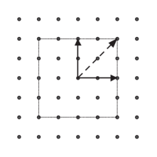
Figure 1: Two-dimensional fermionic lattice with box $B_{2}$ (see proof of Thm. 2). The interactions along $e_{1}$ and $e_{2}$ (solid arrows) are used to simulate the interactions in the direction $2(e_{1}+e_{2})$ (dashed arrow).

Proof We start with an odd number of fermions, $m=2n+1$. For the proof we will consider interactions with a maximal interaction range in each direction $e_{i}$ of the lattice. To do so, we define for every integer $z\in\mathbb{N}$ the $d$-dimensional cube of edge length $2z$, $B_{z}=\{v\in\mathbb{Z}_{m}^{d}|\,\|v\|_{\infty}\leq z\}$. Then a Hamiltonian $H^{(v^{(z)})}$ where $v^{(z)}=(v^{(z)}_{1},\ldots,v^{(z)}_{d})\in B_{z}$ couples a given lattice site $s$ only with sites which lie in a cube of edge size $2z$ with $s$ in its center. We will show by induction over $z$ that $H_{X}^{(v)}$ and $H_{W}^{(v)}$ can be simulated. We start with a minimal edge length of 2, i.e. $z=1$ and define $\mathcal{N}_{v}=\{i\,|\,|v_{i}|=1\}$ with cardinality $|\mathcal{N}_{v}|$. We will show that $H_{X}^{(v^{(1)})},H_{W}^{(v^{(1)})}$ can be simulated for $|\mathcal{N}_{v^{(1)}}|=1,\ldots,d$, i.e., for an arbitrary number of non-vanishing components of the vector $v^{(1)}$. For $|\mathcal{N}_{v^{(1)}}|=1$, the vector $v^{(1)}$ has only one non-vanishing component $v^{(1)}=\pm e_{i}$, and the situation is as the one of theorem 1. Hence $H_{X}^{(\pm e_{i})}$ and $H_{W}^{(\pm e_{i})}$ can be simulated for arbitrary $i$. Now let $|\mathcal{N}_{v^{(1)}}|=r>1$, $j\in\mathcal{N}_{v^{(1)}}$, i.e. we want to simulate an interaction in the direction of the diagonals as depicted in figure 1. As $|\mathcal{N}_{v^{(1)}-v^{(1)}_{j}e_{j}}|=r-1$ we know by induction over the cardinality of $\mathcal{N}_{v^{(1)}}$ that $H_{W}^{(v^{(1)}-v^{(1)}_{j}e_{j})}$ can be simulated. Then we get $H_{X}^{(v^{(1)})}$ as

$$[H_{W}^{(-v^{(1)}_{j}e_{j})},H_{W}^{(v^{(1)}-v^{(1)}_{j}e_{j})}]=H_{X}^{(v^{(1)})},$$

and $H_{W}^{(v^{(1)})}$ can be obtained according to theorem 1. Now we consider boxes with edge length bigger than 2 assuming that $H_{X}^{(v^{(z)})}$ and $H_{W}^{(v^{(z)})}$ can be constructed for all $v^{(z)}\in B_{z}$, and let $v^{(z+1)}=(v_{1}^{(z+1)},\ldots,v_{1}^{(z+1)})\in B_{z+1}$. First we show that there exist $p^{(z)},q^{(z)}\in B_{z}$ such that $p^{(z)}+q^{(z)}=v^{(z+1)},p^{(z)}-q^{(z)}\in B_{z}$ (see figure 2). Therefore we define the set $\mathcal{Z}_{v}=\{i||v_{i}^{(z+1)}|=z+1\}$. If we take $q^{(z)}=\sum_{i\in\mathcal{Z}_{v}}\frac{v_{i}}{|v_{i}|}e_{i}$ and $p^{(z)}=v^{(z+1)}-q^{(z)}$ then by definition $p^{(z)},q^{(z)}\in B_{z}$ and $p^{(z)}+q^{(z)}=v^{(z+1)}$. As for all $i\in\mathcal{Z}_{v}$ we have $|(p^{(z)}-q^{(z)})_{i}|=(|v_{i}|-2)\leqq z-1$ and for all $i\notin\mathcal{Z}_{v}$ we have $|(p^{(z)}-q^{(z)})_{i}|=(|v_{i}|)\leqq z$, it follows that $p^{(z)}-q^{(z)}\in B_{z}$. Using now the commutator relation

$$[H_{X}^{(q^{(z)})},H_{W}^{(p^{(z)})}]=2(H_{W}^{(v^{(z+1)})}-H_{W}^{(p^{(z)}-q^{(z)})}),$$

(see Eq.(37)) we obtain that $H_{W}^{(v^{(z+1)})}$ can be simulated, and from (35) we know that we also get $H_{X}^{(v^{(z+1)})}$.
Now consider the case where $m=2n$. If $x_{i}=-y_{i},w_{0}\neq-\tilde{w}_{i}\;\forall i$, we can simulate $H_{X}^{(ke_{i})}$ and $H_{X}^{(ke_{i})}$ for all $i$ and $k$ according to theorem 1 (2c). Like in the case $m=2n+1$ we can simulate $H_{X}^{(kv^{(1)})}$ for all $v^{(1)}\in B_{1}$, but according to theorem 1 (2b) simulating $H_{W}^{(kv^{(1)})}$ seems not to be possible. So we include these nearest-neighbor interactions in our initial set. The rest of the proof is then like in the case $m=2n+1$, and we see that the space $\mathcal{R}$ can be simulated. $\Box$

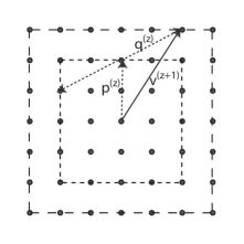
Figure 2: Boxes $B_{z}$ and $B_{z+1}$. Any vector $v^{(z+1)}\in B_{z+1}$ can be decomposed into a sum of vectors from $B_{z}$, i.e., $v^{(z+1)}=p^{(z)}+q^{(z)}$ where $p^{(z)},q^{(z)}\in B_{z}$, such that $q^{(z)}-p^{(z)}\in B_{z}$ (see proofs of Thms. 2 and 4).

V Simulations in bosonic systems

In the following section we will study simulations in translationally invariant bosonic systems using quadratic on-site Hamiltonians and nearest-neighbor interactions. According to Eq. (13) the generators are of the form

$$L=\sigma^{T}\left(\begin{array}[]{cc}-W&Y\\ -X&W\\ \end{array}\right),$$

and their commutator $L^{\prime\prime}=[L,L^{\prime}]$ is given by

$$L^{\prime\prime} = {\small\left(\begin{array}[]{cc}-W^{\prime\prime}&Y^{\prime\prime}\\ -X^{\prime\prime}&W^{\prime\prime T}\\ \end{array}\right)},$$ (42)

$$X^{\prime\prime} = -X^{\prime}(W+W^{T})+X(W^{\prime}+W^{\prime T}),$$ (43)

$$Y^{\prime\prime} = Y(W^{\prime}+W^{\prime T})-Y^{\prime}(W+W^{T}),$$ (44)

$$W^{\prime\prime} = W^{\prime\prime T}=X^{\prime}Y-XY^{\prime}.$$ (45)

As in the fermionic case all commutators obey a symmetry which is in this case $W^{\prime\prime}=W^{\prime\prime T}$ corresponding to reflection symmetry (point symmetry) of the Hamiltonian and we will denote the vector space of all point symmetric Hamiltonians by $\mathcal{P}$. This means that all simulated interactions are point symmetric up to linear combinations of the initial Hamiltonians.

Every generator $L$ of an arbitrary on-site Hamiltonian is of the form

$$E_{(x_{E},y_{E},w_{E})}=\left(\begin{array}[]{cc}-w_{E}\mbox{$1{\bf l}$}&y_{E}\mbox{$1{\bf l}$}\\ -x_{E}\mbox{$1{\bf l}$}&w_{E}\mbox{$1{\bf l}$}\\ \end{array}\right),\;x_{E},y_{E},w_{E}\in\mathbb{R}.$$ (46)

Generators corresponding to a nearest-neighbor interaction along an axis $e_{i}$ are of the form

$$L^{(e_{i})}=\left(\begin{array}[]{cc}-W&Y\\ -X&W^{T}\\ \end{array}\right)=$$ (49)

$$\left(\begin{array}[]{cc}-wM^{(e_{i})}+\tilde{w}M^{(-e_{i})}&yM^{(e_{i})}_{+}\\ xM^{(e_{i})}_{+}&\tilde{w}M^{(e_{i})}+wM^{(-e_{i})}\\ \end{array}\right),$$ (52)

where $x,y,w,\tilde{w}\in\mathbb{R}$ and $M^{(v)}$ has been defined in (19).
We define $L_{W}^{(v)}=\big{(}-M_{+}^{(v)}\big{)}\oplus M_{+}^{(v)}$ and

$$L_{X}^{(v)}=\left(\begin{array}[]{cc}0&0\\ -M_{+}^{(v)}&0\\ \end{array}\right),\;L_{Y}^{(v)}=\left(\begin{array}[]{cc}0&M_{+}^{(v)}\\ 0&0\\ \end{array}\right),$$ (53)

where the indices $X,Y$ and $W$ correspond to a non-zero $X$-, $Y$- and W-block respectively.

V.1 Simulations in one-dimensional bosonic systems

In this section we show that for one-dimensional bosonic systems an arbitrary nearest-neighbor interaction is complete for simulating the vector space $\mathcal{P}$ (i.e. $W=W^{T}$) when supplemented by all on-site Hamiltonians.

Theorem 3

Consider bosonic systems with quadratic Hamiltonians on a one-dimensional translationally invariant lattice with periodic boundary conditions. The set of all possible one-mode transformations $E_{(x_{E},y_{E},w_{E})}$ in (46) together with one arbitrary nearest-neighbor interaction given by $L$ in Eq.(49) is universal for simulating the space $\mathcal{P}$ of all point symmetric interactions.

Proof First we will show that an arbitrary interaction with $X=Y=0,W=W^{T}$ can be brought from the $W$-block in the $X$ and $Y$-block:

$$\left[\left(\begin{array}[]{cc}-W&0\\ 0&W\\ \end{array}\right),\left(\begin{array}[]{cc}0&-\frac{1}{2}\\ 0&0\\ \end{array}\right)\right] = \left(\begin{array}[]{cc}0&W\\ 0&0\\ \end{array}\right),$$ (60)

$$\left[\left(\begin{array}[]{cc}-W&0\\ 0&W\\ \end{array}\right),\left(\begin{array}[]{cc}0&0\\ -\frac{1}{2}&0\\ \end{array}\right)\right] = \left(\begin{array}[]{cc}0&0\\ -W&0\\ \end{array}\right).$$ (67)

Thus it is sufficient to show that an arbitrary $W$-block can be obtained. Let us start with a nearest-neighbor interaction of the form $L_{Y}^{(e_{1})}$. As

$$[L_{Y}^{(e_{1})},E_{(1,0,0)}]=L_{W}^{(e_{1})}$$

we also get $L_{X}^{(e_{1})}$ according to (60). Now $[L_{Y}^{(e_{1})},L_{X}^{(e_{1})}]-2E_{(0,0,1)}=L_{W}^{(2e_{1})},$ so that we also get $L_{X}^{(2e_{1})}$ and $L_{Y}^{(2e_{1})}$. As $[L_{Y}^{(ke_{1})},L_{X}^{(e_{1})}]=L_{W}^{((k+1)e_{1})}+L_{W}^{((k-1)e_{1})}$ we can simulate $\mathcal{P}$.
Finally it remains to show that we can get $L_{Y}^{(e_{1})}$ from an arbitrary nearest-neighbor interaction. If $y\neq 0$ in (49), then $[[L^{(e_{1})},E_{(0,0,1/2)}],E_{(-1,0,0)}]=yL_{W}^{(e_{1})}$ so that we get $L_{Y}^{(e_{1})}$ according to (60). If $y=0,x\neq 0$, then $[[L^{(e_{1})},E_{(0,0,1/2)}],E_{0,1,0}]=xL_{W}^{(e_{1})}$ and we get $L_{Y}^{(e_{1})}$ as before. If $x=y=0,w\neq 0$, then $[L^{(e_{1})},E_{(0,-1,0)}]=(w+\tilde{w})L_{Y}^{(e_{1})}.$ $\Box$

V.2 Simulations in $d$-dimensional bosonic systems

The following generalizes the previous result to cubic lattices in arbitrary spatial dimensions in cases where nearest neighbor interactions along all axes and diagonals are available.

Theorem 4

Consider a system of bosonic modes on a $d$-dimensional translationally invariant lattice with periodic boundary conditions. The set of all on-site transformations together with all nearest-neighbor interactions corresponding to $L^{(\sum_{i}c_{i}e_{i})},c_{i}\in\{0,\pm 1\},i=1\ldots,d$ with $L$ as in Eq.(49) is complete for simulating the space $\mathcal{P}$ of all possible point symmetric interactions.

Proof Like in the $d$-dimensional fermionic case let $B_{z}=\{v|\|v\|_{\infty}\leq z\},z\in\mathbb{N},v^{(z)}\in B_{z}$. ¿From Thm. 3 we know that it is sufficient to show that $L_{W}^{(v)}$ can be simulated for arbitrary $v$. By induction over $z$ we will show that $L_{W}^{(v^{(z)})}$ can be simulated for all $v^{(z)}\in B_{z}$. For $z=1$ we know from Thm. 3 that all interactions described by $v^{(1)}\in B_{1}$ can be simulated as we have chosen our initial Hamiltonians appropriately. Now assume that $L_{W}^{(v^{(z)})}$ can be simulated for all $v^{(z)}\in B_{z}$, and let $v^{(z+1)}\in B_{z+1}$. Then there exist $p^{(z)},q^{(z)}\in B_{z}$ such that $p^{(z)}+q^{(z)}=v^{(z+1)},p^{(z)}-q^{(z)}\in B_{z}$ (see figure 2). As

$$[L_{X}^{(p^{(z)})},L_{Y}^{(q^{(z)})}]=L_{W}^{(v^{(z+1)})}-L_{W}^{(p^{(z)}-q^{(z)})},$$

we can simulate $L_{W}^{(v^{(z+1)})}$. $\Box$

VI Simulations in spin systems

In this section we will consider translationally invariant quantum lattice systems where a $D$-dimensional Hilbert space is assigned to each of the sites. We refer to these systems as spins although, of course, the described degrees of freedom do not have to be spin-like. The main result of this section is that within the translationally invariant setting universal sets of interactions cannot exist. These results are based on the following Lemma involving Casimir operators, i.e., operators which commute with every element of the Lie algebra FultonHarris ; Cornwell :

Lemma 5

Consider a Lie-Algebra $\mathcal{L}$ and subalgebra $\mathcal{L}^{\prime}=[\mathcal{L,L}]$. Let $\mathcal{S_{L}}$ be a set of generators for $\mathcal{L}$ and $C$ a Casimir operator of $\mathcal{L}$ fulfilling

$$\mbox{tr}[CG]=0\;\forall G\in\mathcal{S_{L}}\setminus\mathcal{L}^{\prime}.$$ (68)

Then for every $K\in\mathcal{L}$ we have that $\mbox{tr}[CK]=0$.

Proof Every $K\in\mathcal{L}$ can be written as

$$K=\sum_{L\in\mathcal{L}^{\prime}}\alpha_{L}L+\sum_{G\in\mathcal{S_{L}}\setminus\mathcal{L}^{\prime}}\beta_{G}G\;,\ \ \alpha_{L},\beta_{G}\in\mathbb{C}.$$ (69)

Since we can write any $L\in\mathcal{L}^{\prime}$ as $L=[L_{1},L_{2}]$, $L_{i}\in\mathcal{L}$ we have that

$$\mbox{tr}[CL]=\mbox{tr}[C[L_{1},L_{2}]]=\mbox{tr}[[CL_{1},L_{2}]]=0$$

where we have used that $C$ is a Casimir operator, i.e., $\forall L\in\mathcal{L}:[C,L]=0$. Hence if we take the trace of Eq.(69) with $C$ we get

$$\mbox{tr}[CK]=\sum_{G\in\mathcal{S_{L}}\setminus\mathcal{L}^{\prime}}\beta_{G}\mbox{tr}[CG]$$

which vanishes according to the assumption in Eq.(68). $\Box$

Let us now exploit Lemma 5 in the translationally invariant setting in order to rule out the universality of interactions corresponding to certain sets of generators $\mathcal{S_{L}}$. The following results are stated for one-dimensional systems but they can be applied to $d$-dimensional lattices by grouping sites in $d-1$ spatial dimensions.

We use Casimir operators of the form

$$C=\sum_{k=1}^{m}\gamma_{k}T^{k}\;,\quad\gamma_{k}\in\mathbb{C}\;,$$ (70)

where $T|i_{1},i_{2},\ldots,i_{m}\rangle=|i_{2},i_{3},\ldots,i_{m},i_{1}\rangle$ is the translation operator which shifts the lattice by one site. To simplify notation we define an operator

$$\tau(X)=\sum_{j=1}^{m}T^{j}XT^{\dagger j}\;,$$ (71)

which symmetrizes any operator $X$ with respect to the translation group. If $X$ does not act on the entire lattice we will slightly abuse notation and write $X$ instead of $X\otimes\mbox{$1{\bf l}$}\otimes\cdots\otimes\mbox{$1{\bf l}$}$.

Theorem 6

Consider a translationally invariant spin system on a ring of length $m$. If $f$ is a non-trivial factor of $m$ then there is no universal set of Hamiltonians with interaction range smaller than $f$ which generates all translationally invariant interactions. In particular if $m$ is even, nearest-neighbor interactions cannot generate all next-to-nearest neighbor Hamiltonians.

Proof Let us introduce a basis of the Lie algebra $su_{D^{m}}$ of the form $i\sigma_{j_{1}}\otimes\cdots\otimes\sigma_{j_{m}}$, $j_{k}\in\mathbb{Z}_{D^{2}}$ where $\sigma_{k}$ is traceless except for $\sigma_{0}=\mbox{$1{\bf l}$}$ and $\mbox{tr}[\sigma_{k}^{2}]=2$ for all $k>0$. For $D=2$ these are the Pauli matrices

$$\sigma_{1}=\left(\begin{array}[]{cc}0&1\\ 1&0\\ \end{array}\right),\;\sigma_{2}=\left(\begin{array}[]{cc}0&-i\\ i&0\\ \end{array}\right),\;\sigma_{3}=\left(\begin{array}[]{cc}1&0\\ 0&-1\\ \end{array}\right),$$ (72)

and for $D>2$ we can simply choose all possible embeddings thereof. Let $m=f\cdot f^{\prime}$ and consider a Casimir operator of the form in Eq.(70) with $\gamma_{k}=\delta_{k,f}$, i.e., $C=T^{f}$.

We first show that for every Hamiltonian $H\in su_{D^{m}}$ with interaction range smaller than $f$ we have $\mbox{tr}[CH]=0$. To see this note that the shift operator $T^{f}$ contracts the trace of a tensor product as

$$\mbox{tr}\big{[}T^{f}\sigma_{j_{1}}\otimes\cdots\otimes\sigma_{j_{m}}\big{]}=\prod_{\beta=1}^{f}\mbox{tr}\left[\prod_{\alpha=0}^{f^{\prime}-1}\sigma_{j_{(\beta+\alpha f)}}\right].$$ (73)

In order to arrive at formula (73) expand the translation operator $T^{f}$ in the computational basis

$$T^{f}=\sum_{i_{1},\ldots,i_{m}}|i_{1}\ldots i_{m}\rangle\langle i_{m-(f-1)}i_{m-(f-2)}\ldots i_{1}\ldots i_{m-f}|$$

in order to get

$$\mbox{tr}\big{[}T^{f}\sigma_{j_{1}}\otimes\cdots\otimes\sigma_{j_{m}}\big{]}=\hskip 142.26378pt$$

$$\sum_{i_{1},\ldots,i_{m}}\langle i_{m-(f-1)}|\sigma_{j_{1}}|i_{1}\rangle\langle i_{m-(f-2)}|\sigma_{j_{2}}|i_{2}\rangle\ldots\langle i_{m-f}|\sigma_{j_{m}}|i_{m}\rangle.$$

Rearranging the order of the factors and using $(f^{\prime}-1)f=m-f$ leads to

$$\prod_{\beta=1}^{f}\sum_{i_{\beta},i_{f+\beta},\ldots}\langle i_{m-(f-\beta)}|\sigma_{j_{\beta}}|i_{\beta}\rangle\langle i_{\beta}|\sigma_{j_{(f+\beta)}}|i_{f+\beta}\rangle\cdot\ldots\cdot$$

$$\langle i_{(f^{\prime}-2)f+\beta}|\sigma_{j_{((f^{\prime}-1)f+\beta)}}|i_{(f^{\prime}-1)f+\beta}\rangle=$$

$$\prod_{\beta=1}^{f}\mbox{tr}\left[\prod_{\alpha=0}^{f^{\prime}-1}\sigma_{j_{(\beta+\alpha f)}}\right]\hskip 128.0374pt$$

If the interaction range of $H$ is smaller than $f$ then it can be decomposed into elements of the form $\tau(\sigma_{i_{1}}\otimes\cdots\otimes\sigma_{i_{f}})$. Since $\sigma_{k}$ is traceless for all $k>0$, all these terms amount to a vanishing trace in Eq.(73) so that we have indeed $\mbox{tr}[CH]=0$. This means we can apply Lemma 5 to the set $\mathcal{S_{L}}$ corresponding to all interactions with range smaller than $f$.

Now consider a two-body interaction between site one and site $f+1$ of the form $\tilde{H}=\tau\big{(}\sigma_{j}^{(1)}\sigma_{j}^{(1+f)}\big{)}$. From Eq.(73) we get

$$\mbox{tr}[C\tilde{H}]=m\mbox{tr}[\sigma_{j}^{(1)}\sigma_{j}^{(1+f)}]\prod_{\beta=2}^{f}\mbox{tr}[\mbox{$1{\bf l}$}]=2mD^{f}$$

such that by Lemma 5 we conclude that $\tilde{H}$ cannot be simulated. $\Box$

The following shows that a universal set of nearest-neighbor interactions cannot exist irrespective of the factors of $m$:

Theorem 7

Consider a ring of length $m$. Then the set $\mathcal{S_{L}}$ corresponding to all on-site Hamiltonians and nearest-neighbor interactions is not universal for simulating all translationally invariant Hamiltonians. In particular for $D=2$ a product Hamiltonian

$$H=\tau\Big{(}\sigma_{j_{1}}\otimes\cdots\otimes\sigma_{j_{m}}\Big{)}$$ (74)

cannot be simulated if $\sigma_{1},\sigma_{2}$ and $\sigma_{3}$ all occur an odd number of times.

Proof We use the Casimir operator $C=T-T^{\dagger}$ and the set of generators $\mathcal{S_{L}}=i\{\tau(\sigma_{k}\otimes\sigma_{l})\}\subset su_{2^{m}}$. As $\mbox{tr}[CG]=0$ for all $G\in\mathcal{S_{L}}$ we can again apply Lemma 5. Consider now the above product Hamiltonian $H$ or if $D>2$ its embedding respectively. Using Eq.(73) with $f=1,f^{\prime}=m$ we obtain

$$\mbox{tr}[CH]=m\mbox{tr}\left[\prod_{k=1}^{m}\sigma_{i_{k}}-\prod_{l=1}^{m}\sigma_{i_{l}}^{T}\right].$$ (75)

Since $\sigma_{i}^{T}=(-1)^{\delta_{i,2}}\sigma_{i}$ and by assumption $\sigma_{2}$ appears an odd number of times we get $\mbox{tr}[CH]=2m\mbox{tr}\big{[}\prod_{k=1}^{m}\sigma_{i_{k}}\big{]}$ which is non-zero iff $\sigma_{1}$ and $\sigma_{3}$ appear and odd number of times as well. $\Box$

Clearly, one can derive other no-go theorems in a similar manner from Lemma 5. However, we end this section by providing some examples of interactions which can be simulated. For this we define $g_{kl}=\tau(\sigma_{k}\otimes\sigma_{l})$.

Theorem 8

Consider a translationally invariant system of $m$ qubits ($D=2$) on a ring. By using on-site Hamiltonians and nearest-neighbor interactions the following interactions can be simulated:

$$\tau(\sigma_{i}\otimes\sigma_{i}\otimes\sigma_{i}),$$ (76)

$$J_{ij}^{(r_{j})} = \tau(\sigma_{i}\otimes\sigma_{j}\otimes\ldots\sigma_{j}\otimes\sigma_{i}),$$ (77)

where $i,j\in\{1,2,3\}$ and $r_{j}$ denotes the number of $\sigma_{j}$ matrices. Moreover, for $m=5$ one can simulate next-to-nearest neighbor interactions of the form $N_{i}=\tau(\sigma_{i}\otimes\mbox{$1{\bf l}$}\otimes\sigma_{i}\otimes\mbox{$1{\bf l}$}\otimes\mbox{$1{\bf l}$}).$

Proof We will restrict our proof to the pairs $i=1,j=2$ as the other interactions can be obtained in an analogous way. We start proving (76). The Hamiltonian (76) can be simulated due to $[g_{21},g_{13}]/(2i)=\tau(\sigma_{1}\otimes\sigma_{1}\otimes\sigma_{1})$. For proving (77), we start with $[g_{13},g_{11}]/(2i)=J_{12}^{(1)}$. As $[J_{12}^{(r_{2})},g_{31}]/(2i)=J_{12}^{(r_{2}-1)}-J_{12}^{(r_{2}+1)}$, $J_{12}^{(0)}=g_{11}$, we have shown (77).
Now we will prove that the next-to-nearest neighbor interaction can be achieved for $m=5$, $i=1$ ($i=2,3$ follow similarly). Using (77), we see that $\tau(\sigma_{1}\otimes\sigma_{1}\otimes\sigma_{1}\otimes\sigma_{1}\otimes\mbox{$1{\bf l}$})$ can be simulated, as $[g_{23},J_{21}^{(3)}]/(2i)+J_{(21)}^{(2)}=\tau(\sigma_{1}\otimes\sigma_{1}\otimes\sigma_{1}\otimes\sigma_{1}\otimes\mbox{$1{\bf l}$})$, and similarly we get $\tau(\sigma_{3}\otimes\sigma_{3}\otimes\sigma_{3}\otimes\sigma_{3}\otimes\mbox{$1{\bf l}$})$. As $[[g_{11},g_{23}],g_{32}]/4=2N_{1}-\tau(\sigma_{1}\otimes\sigma_{1}\otimes\sigma_{1}\otimes\sigma_{1}\otimes\mbox{$1{\bf l}$})-\tau(\sigma_{3}\otimes\sigma_{3}\otimes\sigma_{3}\otimes\sigma_{3}\otimes\mbox{$1{\bf l}$})$ we can extract $N_{1}$. $\Box$

VII Conclusions

We have presented a characterization of universal sets of translationally invariant Hamiltonians for the simulation of interactions in quadratic fermionic and bosonic systems given the ability of engineering local and nearest neighbor interactions. Thereby the Lie algebraic techniques of quantum simulation restrict the space of reachable interactions to Hamiltonians with real hopping amplitudes in the case of fermions and to point symmetric interactions in the case of bosons.

For spins the situation appears to be more difficult and a complete characterization of interactions that can be simulated remains to be found. As a first step, we have identified Hamiltonians that cannot be simulated using short range interactions only. Furthermore, we have introduced a technique based on the Casimir operator of the corresponding Lie algebra which allows one to find Hamiltonians that cannot be simulated with a given set of interactions.

In this work we have considered the question of what can be simulated leaving aside the question of the efficiency. In this context it is important to remark the fact that the number of applications of the original Hamiltonians in order to obtain a result bounded by some given error scales polynomially in the Trotter expansion. The scaling with the total number of particles depends on the number of commutators that are required to obtain the Hamiltonian.

Finally, whereas we have shown that it is not possible to perform certain simulations for spin systems it is still possible to perform those simulations by encoding the qubits in a different way.

We thank the Elite Network of Bavaria QCCC, DFG-Forschungsgruppe 635, SFB 631, SCALA and CONQUEST.

References

- (1) R.P. Feynman, Int. J. Theor. Phys. 21, 467 (1982).
- (2) S. Lloyd, Science 273, 1073 (1996); C. Zalka, Proc. Roy. Soc. Lond. A 454, 313 (1998).
- (3) M. Greiner, O. Mandel, T. Esslinger, T.W. Hänsch, I. Bloch, Nature(London) 415, 39 (2002).
- (4) D. Leibfried, R. Blatt, C. Monroe, D. Wineland, Rev.Mod. Phys. 75, 281 (2003).
- (5) D. Porras, J.I. Cirac, quant-ph/0401102; quant-ph/0409015; quant-ph/0601148.
- (6) E. Jane, G. Vidal, W. Dür, P. Zoller, J.I. Cirac, Quant. Inf. Comp. 3(1), 15 (2003).
- (7) D. Jaksch, C. Bruder, J.I. Cirac, C.W. Gardiner, P. Zoller, Phys. Rev. Lett. 81, 3108 (1998).
- (8) D. Deutsch, A. Barenco, A. Ekert, Proc. R. Soc. Lond. A 449, 669 (1995); S. Lloyd, Phys. Rev. Lett., 75, 346 (1995).
- (9) J.L. Dodd, M.A. Nielsen, M.J. Bremner, R.T. Thew, Phys. Rev. A 65, 040301(R) (2002); M.A. Nielsen, M.J. Bremner, J.L. Dodd, A.M. Childs, C.M. Dawson, Phys. Rev. A 66, 022317 (2002).
- (10) M. J. Bremner, J. L. Dodd, M. A. Nielsen, and D. Bacon, Phys. Rev. A 69, 012313 (2004); M. J. Bremner, D. Bacon, M. A. Nielsen, Phys. Rev. A 71, 052312 (2005).
- (11) C.H. Bennett, J.I. Cirac, M.S. Leifer, D.W. Leung, N. Linden, S. Popescu, G. Vidal, Phys. Rev. A 66, 012305 (2002); P.Wocjan, M. Rötteler, D. Janzing, T. Beth, Phys. Rev. A 65, 042309 (2002); P. Wocjan, M. Rötteler, D. Janzing, T. Beth, Quantum Inf. Comput. 2 133 (2002); G. Vidal, J.I. Cirac, Phys. Rev A 66, 022315 (2002).
- (12) W. Fulton, J. Harris, Representation Theory, Graduate Texts in Mathematics 129, Springer (1991).
- (13) J.F. Cornwell, Group Theory in Physics Vol. 1 and 2, Academic Press.
- (14) H.F. Trotter, Proc. Am. Math. soc. 10, 545 (1959); P.R. Chernoff, J. Functional Analysis 2, 238 (1968).
- (15) F. Haussdorff, Ber. Ver. Saechs. Akad. Wiss. Leipzig, Math.-Phys.Kl. 58, 19 (1906); E.B. Dynkin Math. Rev. 11, 80 (1949); E.B. Dynkin, Am. Math. Soc. Transl. 9, 470 (1950).
- (16) E. Lieb, T. Schulz, D. Mattis, Ann. Phys. (N.Y.) 16, 407 (1961).
- (17) H. Araki, ”Bogoliubov tranformation and Fock representation of canonical anticommutator relations” in Operator Algebras and Mathematical Physics, Contemporary Mathematics 62, Iowa City (1987).
- (18) S. Bravyi, Quantum Inf. and Comp. 5, 216 (2005).
- (19) M.M. Wolf, Phys. Rev. Lett. 96, 010404 (2006).
- (20) N. Schuch, J.I. Cirac, M. Wolf, Commun. Math. Phys. 267, 65 (2006).
- (21) K. Audenaert, J. Eisert, M.B. Plenio, R.F. Werner, Phys. Rev. A 66, 042327 (2002).