The mother of all protocols:
Restructuring quantum information’s family tree

Abstract

We give a simple, direct proof of the “mother” protocol of quantum information theory. In this new formulation, it is easy to see that the mother, or rather her generalization to the fully quantum Slepian-Wolf protocol, simultaneously accomplishes two goals: quantum communication-assisted entanglement distillation, and state transfer from the sender to the receiver. As a result, in addition to her other “children,” the mother protocol generates the state merging primitive of Horodecki, Oppenheim and Winter, a fully quantum reverse Shannon theorem, and a new class of distributed compression protocols for correlated quantum sources which are optimal for sources described by separable density operators. Moreover, the mother protocol described here is easily transformed into the so-called “father” protocol whose children provide the quantum capacity and the entanglement-assisted capacity of a quantum channel, demonstrating that the division of single-sender/single-receiver protocols into two families was unnecessary: all protocols in the family are children of the mother.

I Introduction

One of the major goals of quantum information theory is to find the optimal ways to make use of noisy quantum states or channels for communication or establishing entanglement. Quantum Shannon theory attacks the problem in the limit of many copies of the state or channel in question, in which situation the answers often simplify to the point where they can be expressed by relatively compact formulae. The last ten years have seen major advances in the area, including, among many other discoveries, the determination of the classical capacity of a quantum channel H98 ; SW97 , the capacities of entanglement-assisted channels BSST99 ; BSST02 , the quantum capacity of a quantum channel L96 ; S02 ; D05 , and the best ways to use noisy entanglement to extract pure entanglement DW05 or to help send classical information HHHLT01 . Until recently, however, each new problem was solved essentially from scratch and no higher-level structure was known connecting the different results. Harrow’s introduction of the cobit H04 and its subsequent application to the construction of the so-called “mother” and “father” protocols provided that missing structure. Almost all the problems listed above were shown to fall into two families, first the mother and her descendants, and second the father and his DHW04 . Appending or prepending simple transformations like teleportation and superdense coding sufficed to transform the parents into their children.

In this paper, we provide a direct proof of the mother protocol or, more precisely, of the existence of a protocol performing the same task as the mother. In contrast to most proofs in information theory, instead of showing how to establish perfect correlation of some kind between the sender (Alice) and the receiver (Bob), our proof proceeds by showing that the protocol destroys all correlation between the sender and a reference system. Since destruction is a relatively indiscriminate goal, the resulting proof is correspondingly simple. This approach also makes it clear that the mother actually accomplishes more than originally thought. In particular, in addition to distilling entanglement between Alice and Bob, the protocol transfers all of Alice’s entanglement with a reference system to Bob. This side effect is very important in its own right, and a major focus of our paper. To start, it places the state merging protocol of Horodecki, Oppenheim and Winter HOW05 ; HOW05b squarely within the mother’s brood. In addition, it makes it possible to use the mother as a building block for distributed compression. We analyze the resulting protocols, finding they are optimal for sources described by separable density operators, as well as inner and outer bounds on the achievable rate region in general.

We also emphasize a further connection, first identified in D05b , that requires both the state transfer and entanglement distillation capabilities of the mother: the entire protocol allows for a time-reversed interpretation as a quantum reverse Shannon theorem, that is, an efficient simulation of a noisy quantum channel using a noiseless quantum channel along with entanglement.

Finally, the new approach to the mother solves a major problem left unanswered in the original family paper. There, no operational relationship between the mother and father protocols could be identified, but the two were nonetheless connected by a formal symmetry called source-channel duality D05b . This new mother protocol can be directly transformed into the father, resolving the mystery of the two parents’ formal similarity and collapsing the two families into one.

The structure of the paper is as follows. After reviewing the family of quantum protocols in section II and providing, in section III a high-level description of the improved mother, henceforth the fully quantum Slepian-Wolf (FQSW) protocol, we go straight to the statement and proof of the central result of this paper in section IV: a one-shot version of FQSW. The middle section of the paper is devoted to a number of applications of one-shot FQSW. Sections V and VI describe one-shot versions of the “father” and the fully quantum “quantum reverse Shannon” (FQRS) protocol, respectively. The one-shot theorems quickly yield memoryless forms for all three: FQSW in section VII, the father in section VIII and FQRS in section IX. Then we turn to the other highlight of this paper, a treatment of the fully quantum version of the distributed compression problem, which we can solve completely for a large class of sources by providing general inner and outer bounds on the rate region, in section X. In section XI we point out that the FQSW protocol allows for efficient encoding via Clifford operations, after which we conclude. An appendix collects useful facts on typical subspaces.

Notation: For a quantum system $A$, let $d_{A}=\dim A$. For two quantum systems $A$ and $A^{\prime}$, let $F^{A}$ be the operator that swaps the two systems. An operator acting on a subsystem is freely identified with its extension (via tensor product with the identity) to larger systems. $\Pi^{A}_{+}$ denotes the projector onto the symmetric subspace of $A\otimes A^{\prime}$ and $\Pi^{A}_{-}$ the projector onto the antisymmetric subspace of $A\otimes A^{\prime}$. Let ${{\mathbb{U}}}(A)$ be the unitary group on $A$. $H(A)_{\varphi}$ is the von Neumann entropy of $\varphi^{A}$, $I(A;B)_{\varphi}=H(A)_{\varphi}+H(B)_{\varphi}-H(AB)_{\varphi}$ is the mutual information between the $A$ and $B$ parts of $\varphi$ and $H(A|B)_{\varphi}=H(AB)_{\varphi}-H(B)_{\varphi}$ the conditional entropy. The symbol $|\Phi\rangle^{AB}$ will be used to represent a maximally entangled state between $A$ and $B$. Logarithms are taken base 2 throughout.

II The family of quantum protocols

The mother protocol is a transformation of a tensor power quantum state $(|\varphi\rangle^{ABR})^{\otimes n}$. At the start, Alice holds the $A$ shares and Bob the $B$ shares. $R$ is a reference system purifying the $AB$ systems and does not participate actively in the protocol. In the original formulation, the mother protocol accomplished a type of entanglement distillation between Alice and Bob in which the only communication permitted was the ability to send qubits from Alice to Bob. The transformation can be expressed concisely in the resource inequality formalism as

$$\langle\varphi^{AB}\rangle+\frac{1}{2}I(A;R)_{\varphi}\,[q\rightarrow q]\geq\frac{1}{2}I(A;B)_{\varphi}\,[qq].$$ (1)

We will informally explain the resource inequalities used here, but the reader is directed to DHW05 for a rigorous treatment. $[q\rightarrow q]$ represents one qubit of communication from Alice to Bob and $[qq]$ represents an ebit shared between them. In words, $n$ copies of the state $\varphi$ shared between Alice and Bob can be converted into $I(A;B)_{\varphi}$ EPR pairs per copy provided Alice is allowed to communicate with Bob by sending him qubits at rate $I(A;R)_{\varphi}$ per copy. Small imperfections in the final state are permitted provided they vanish as $n$ goes to infinity.

In this paper, we prove a stronger resource inequality which we call the fully quantum Slepian-Wolf (FQSW) inequality. The justification for this name will become apparent in Section X, where we study its applicability to distributed compression, solved classically by Slepian and Wolf SW71 . The inequality states that starting from state $(|\varphi\rangle^{ABR})^{\otimes n}$ and using only quantum communication at the rate $\mbox{$\frac{1}{2}$}I(A;R)_{\varphi}$ from Alice to Bob, they can distill EPR pairs at the rate $\mbox{$\frac{1}{2}$}I(A;B)_{\varphi}$ and produce a state approximating $(|\psi\rangle^{R\widehat{B}})^{\otimes n}$, where $\widehat{B}$ is held by Bob and $\varphi^{R}=\psi^{R}$. That is, Alice can transfer her entanglement with the reference system $R$ to Bob while simultaneously distilling ebits with him. A graphical depiction of this transformation is given in Figure 1. The process can also be expressed as a resource inequality in the following way:

$$\langle W^{S\rightarrow AB}\mathrel{\mathop{\mathchar 58\relax}}\varphi^{S}\rangle+\frac{1}{2}I(A;R)_{\varphi}\,[q\rightarrow q]\geq\frac{1}{2}I(A;B)_{\varphi}\,[qq]+\langle{\operatorname{id}}^{S\rightarrow\widehat{B}}\mathrel{\mathop{\mathchar 58\relax}}\varphi^{S}\rangle$$ (2)

This inequality makes use of the concept of a relative resource. A resource of the form $\langle\mathcal{N}\mathrel{\mathop{\mathchar 58\relax}}\rho^{S}\rangle$ is a channel with input system $S$ that is guaranteed to behave like the channel $\mathcal{N}$ provided the reduced density operator of the input state on $S$ is $\rho^{S}$. In the inequality, $W^{S\rightarrow AB}$ is an isometry taking the $S$ system to $AB$. Thus, on the left hand side of the inequality, a state is distributed to Alice and Bob while on the right hand side, that same state is given to Bob alone. Transforming the first situation into the second means that Alice transfers her portion of the state to Bob.

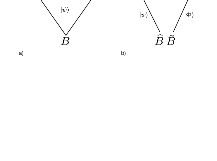
Figure 1: a) The starting point for the FQSW protocol, a pure tripartite entangled state $|\psi\rangle=(|\varphi\rangle^{ABR})^{\otimes n}$. b) After execution of the protocol, Alice’s portion of the original tripartite state has been transferred to Bob, so that Bob holds a purification of the unchanged reference system in his register $\widehat{B}$. He also shares pure state entanglement with Alice in the form of the state $|\Phi\rangle$.

Since the relationship of the mother to entanglement distillation and communication supplemented using noisy entanglement is explained at length in the original family paper, we will not describe the connections here. The FQSW inequality is stronger than the mother, however, and leads to more children. In particular, if the entanglement produced at the end of the protocol is then re-used to perform teleportation, we get the following resource inequality:

$$\langle W^{S\rightarrow AB}\mathrel{\mathop{\mathchar 58\relax}}\varphi^{S}\rangle+H(A|B)_{\varphi}\,[q\rightarrow q]+I(A;B)_{\varphi}\,[c\rightarrow c]\geq\langle{\operatorname{id}}^{S\rightarrow\widehat{B}}\mathrel{\mathop{\mathchar 58\relax}}\varphi^{S}\rangle,$$ (3)

which is known as the state merging primitive HOW05 . It is of note both because it is a useful building block for multiparty protocols HOW05 ; HOW05b ; YHD06 and because it provides an operational interpretation of the conditional entropy $H(A|B)_{\varphi}$ as the number of qubits Alice must send Bob in order to transfer her state to him, ignoring the classical communication cost.

On the other side of the family there is the father protocol. In contrast to the mother, in which Alice and Bob share a mixed state $(\varphi^{AB})^{\otimes n}$, for the father protocol they are connected by a noisy channel ${\cal N}^{A^{\prime}\rightarrow B}$. Let $U^{A^{\prime}\rightarrow BE}$ be a Stinespring dilation of ${\cal N}$ with environment system $E$, such that ${\cal N}(\rho)=\operatorname{Tr}_{E}U\rho U^{\dagger}$, and define $|\varphi\rangle^{ABE}=U^{A^{\prime}\rightarrow BE}|\varphi\rangle^{AA^{\prime}}$ for a pure state $|\varphi\rangle^{AA^{\prime}}$. The resource inequality is

$$\langle{\cal N}^{A^{\prime}\rightarrow B}\rangle+\frac{1}{2}I(A;E)_{\varphi}\,[qq]\geq\frac{1}{2}I(A;B)_{\varphi}\,[q\rightarrow q].$$ (4)

Thus, Alice and Bob use pre-existing shared entanglement and the noisy channel to produce noiseless quantum communication. Comparing Eq. (4) to the mother, Eq. (1), reveals the two to be strikingly similar: to go from one to the other it suffices to replace channels by states and vice-versa, as well as replace the reference $R$ by the environment $E$. This formal symmetry is known as source-channel duality D05b . Just as the mother can be strengthened to the fully quantum Slepian-Wolf protocol, there is a fully coherent version of the father known as the feedback father D05b .

The relationships between different protocols are sketched as a family tree in Figure 2.

Figure 2: Partial quantum information theory family tree. The symbols ß  and æ  represent the “old” mother and father protocols from DHW04 and arrows indicate that a protocol accomplishing the task at the start of the arrow can be transformed into a protocol accomplishing the task at the end. The relationships between ß  , æ  and their children are discussed in detail in DHW04 ; DHW05 . “QMAC” refers to the task of sending quantum data through a quantum multiple access channel HOW05 ; YDH05 , “broadcast” the task of sending quantum data through a quantum broadcast channel YHD06 and the environment-assisted quantum capacity is discussed in SVW05 .

III The fully quantum Slepian-Wolf protocol

The input to the fully quantum Slepian-Wolf protocol is a quantum state, $(|\varphi\rangle^{RAB})^{\otimes n}$, and the output is also a quantum state, $|\Phi\rangle^{A_{2}\tilde{B}}(|\varphi\rangle^{R\widehat{B}})^{\otimes n}$. $A_{2}$ is a quantum system held by Alice while both $\tilde{B}$ and $\widehat{B}$ are held by Bob. $|\Phi\rangle^{A_{2}\tilde{B}}$ therefore represents a maximally entangled state shared between Alice and Bob. The size of the $A_{2}$ system is $nI(A;B)_{\varphi}-o(n)$ qubits. The steps in the protocol that transform the input state to the output state are as follows:

1. Alice performs Schumacher compression on her system $A^{n}$. The output space $A_{S}$ factors into two subsystems $A_{1}$ and $A_{2}$ with $\log d_{A_{1}}=nI(A;R)+o(n)$.

2. Alice applies a unitary transformation $U_{A}$ to $A_{S}$ and then sends $A_{1}$ to Bob.

3. Bob applies an isometry $V_{B}$ taking $A_{1}B^{n}$ to $\widehat{B}\tilde{B}$.

It remains to specify which transformations $U_{A}$ and $V_{B}$ Alice and Bob should apply, as well as a more precise bound on $d_{A_{1}}$. Observe that each step in the protocol is essentially non-dissipative. Since essentially no information is leaked to the environment at any step, Bob will hold a purification of the $A_{2}R^{n}$ system after step $2$, regardless of the choice of $U_{A}$. Because all purifications are equivalent up to local isometric transformations of the purifying space, it therefore suffices to ensure that the reduced state on $A_{2}R^{n}$ approximates $\Phi^{A_{2}}\otimes(\varphi^{R})^{\otimes n}$ after step $2$. Bob’s isometry $V_{B}$ will be the one taking the purification he holds upon receiving $A_{2}$ to the one approximating $|\Phi\rangle^{A_{2}\tilde{B}}(|\varphi\rangle^{R\widehat{B}})^{\otimes n}$.

From this perspective, the operation $\rho\rightarrow\operatorname{Tr}_{A_{1}}(U_{A}\,\rho\,U_{A}^{\dagger})$ should be designed to destroy the correlation between $A_{2}$ and $R^{n}$: the mother will succeed provided the state on $A_{2}\otimes R^{n}$ is a product state and $A_{2}$ is maximally mixed. The operation $U_{A}$ does not itself destroy the correlation; the partial trace over $A_{1}$ does that. $U_{A}$ should therefore be chosen in order to ensure that tracing over $A_{1}$ should be maximally effective. Because one qubit can carry at most two bits of information, tracing over a qubit can reduce mutual information by at most two bits. The starting state $(\varphi^{AR})^{\otimes n}$ has $nI(A;R)_{\varphi}$ bits of mutual information, which means that $A_{1}$ must consist of at least $\mbox{$\frac{n}{2}$}I(A;R)_{\varphi}$ qubits. We will see that by choosing $U_{A}$ randomly according to the Haar measure we will come close to achieving this rate.

The result is similar in spirit to a recent result of Groisman et al. that demonstrated that in order to destroy correlation in the state $\varphi$ by discarding classical information instead of quantum, Alice must discard twice as large a system as she does here: $I(A;R)_{\varphi}$ cbits per copy GPW05 . In fact, it is clear that we can derive that result from ours: after Alice’s unitary, the state remaining between $A_{2}$ and $R$ is almost a product since Alice’s entanglement with the reference gets transferred to Bob, so Alice only needs to discard the system $A_{1}$ of roughly $\frac{n}{2}I(A;R)$ qubits, which she can do by erasing it entirely via random Pauli operations, at randomness cost amounting to $I(A;R)$ cbits per copy.

IV Fully quantum Slepian-Wolf: one-shot version

While the tensor power structure of $(|\varphi\rangle^{ABR})^{\otimes n}$ allows the fully quantum Slepian-Wolf inequality (2) to be expressed conveniently in terms of mutual information quantities, our approach allows us to treat arbitrary input states without such structure as well. In this section, we will prove a general “one-shot” version of the fully quantum Slepian-Wolf result that leads quickly to inequality (2) in the special case where the input state is a tensor power.

For this section, we will therefore dispense with $|\varphi\rangle^{\otimes n}$ and instead study a general state $|\psi\rangle^{ABR}$ shared between Alice, Bob and the reference system. We also eliminate the Schumacher compression step: assume that $A$ has been decomposed into subsystems $A_{1}$ and $A_{2}$ satisfying $d_{A}=d_{A_{1}}d_{A_{2}}$.

The following inequality is the one-shot version of fully quantum Slepian-Wolf:

Theorem IV.1 (One-shot, fully quantum Slepian-Wolf bound)

There exist isometries $U^{A\rightarrow A_{1}A_{2}}$ and $V^{A_{1}B\rightarrow\widehat{B}\tilde{B}}$ such that

$$\Big{\|}(V\circ U)\psi^{RAB}(V\circ U)^{\dagger}-\psi^{R\widehat{B}}\otimes\Phi^{A_{2}\tilde{B}}\Big{\|}_{1}\leq 2\left[\frac{2d_{A}d_{R}}{d^{2}_{A_{1}}}\Big{\{}\operatorname{Tr}[(\psi^{AR})^{2}]+2\operatorname{Tr}[(\psi^{A})^{2}]\operatorname{Tr}[(\psi^{R})^{2}]\Big{\}}\right]^{1/4},$$

where $W^{\widehat{B}\rightarrow AB}|\psi\rangle^{R\widehat{B}}=|\psi\rangle^{RAB}$ for some isometry $W$.

The protocol corresponding to the above theorem consists of Alice performing $U$, sending the $A_{1}$ system to Bob, and Bob performing $V$. The number of qubit channels used up is $\log d_{A_{1}}$ whereas the number of ebits distilled is $\log d_{A_{2}}=\log d_{A}-\log d_{A_{1}}$.

The main ingredient is the following decoupling theorem.

Theorem IV.2 (Decoupling)

Let $\sigma^{A_{2}R}(U)=\operatorname{Tr}_{A_{1}}[(U\otimes I^{R})\psi^{AR}(U^{\dagger}\otimes I^{R})]$ be the state remaining on $A_{2}R$ after the unitary transformation $U$ has been applied to $A=A_{1}A_{2}$. Then

$$\int_{{{\mathbb{U}}}(A)}\Big{\|}\sigma^{A_{2}R}(U)-\sigma^{A_{2}}(U)\otimes\sigma^{R}(U)\Big{\|}_{1}^{2}\,dU\leq\frac{d_{A}d_{R}}{d_{A_{1}}^{2}}\Big{\{}\operatorname{Tr}[(\psi^{AR})^{2}]+\operatorname{Tr}[(\psi^{A})^{2}]\operatorname{Tr}[(\psi^{R})^{2}]\Big{\}}.$$ (5)

The theorem quantifies how distinguishable $\sigma^{A_{2}R}(U)$ will be from its completely decoupled counterpart $\sigma^{A_{2}}(U)\otimes\sigma^{R}(U)$ if $U$ is chosen at random according to the Haar measure. As a first observation, note that as $d_{A_{1}}$ grows, the two states become progressively more indistinguishable. Also, the upper bound on the right hand side is expressed entirely in terms of the dimensions of the spaces involved and the purities $\operatorname{Tr}[(\psi^{AR})^{2}]$, $\operatorname{Tr}[(\psi^{A})^{2}]$ and $\operatorname{Tr}[(\psi^{R})^{2}]$. In the tensor power source setting, both dimensions and purities can be tightly bounded by functions of the corresponding entropies, but in the one-shot setting they must be distinguished.

In many situations of interest, the first term in the upper bound dominates. In such cases, in order to assure a good approximation, it suffices that

$$\log d_{A_{1}}\gg\frac{1}{2}\Big{[}\log d_{A}+\log d_{R}+\log\operatorname{Tr}[(\psi^{AR})^{2}]\Big{]}.$$ (6)

This expression plays the role of the $\mbox{$\frac{1}{2}$}I(A;R)=\mbox{$\frac{1}{2}$}[H(A)+H(R)-H(AR)]$ from the FQSW resource inequality (2) in the one-shot setting.

According to the proof strategy outlined in the previous section, if $\sigma^{A_{2}R}(U)$ is close to $\sigma^{A_{2}}(U)\otimes\sigma^{R}(U)$, then $\sigma^{A_{2}R}(U)$ has a purification which is itself close to a product state. This argument will be made quantitative in the proof of Theorem IV.1.

The proof of the Theorem IV.2 is quite straightforward. We will evaluate the corresponding average over the unitary group exactly for the Hilbert-Schmidt norm and then use simple inequalities to extract inequality (5). The evaluations of the relevant averages are mechanical but slightly lengthy calculations. The reader is advised that the proofs of lemmas IV.3, IV.4 and IV.5 are devoted entirely to the calculation of such averages and can be skipped on a first reading without impairing understanding of the rest of the paper.

Before starting in earnest, we perform a calculation whose result will be re-used several times. Recall from the notation summary in the introduction that $F^{A_{2}R}$ is the operator that swaps the composite system $A_{2}R$ with a duplicate composite system $A_{2}^{\prime}R^{\prime}$, and that $\Pi^{A}_{+(-)}$ is the projector onto the (anti-)symmetric subspace of $A$.

Lemma IV.3

$$\int_{{{\mathbb{U}}}(A)}(U^{\dagger}\otimes U^{\dagger}\otimes I^{RR^{\prime}})F^{A_{2}R}(U\otimes U\otimes I^{RR^{\prime}})\,dU=[p\Pi^{A}_{+}+q\Pi^{A}_{-}]\otimes F^{R},$$ (7)

where

$$p=\frac{d_{A_{1}}+d_{A_{2}}}{d_{A}+1}\quad\mbox{and}\quad q=\frac{d_{A_{1}}-d_{A_{2}}}{d_{A}-1}.$$ (8)

Proof.

Let $X$ be Hermitian. By Schur’s Lemma,

$$\int_{{{\mathbb{U}}}(A)}(U^{\dagger}\otimes U^{\dagger})X(U\otimes U)\,dU=\alpha_{+}(X)\Pi^{A}_{+}+\alpha_{-}(X)\Pi^{A}_{-},$$ (9)

with the coefficients $\alpha_{\pm}(X)=\operatorname{Tr}(X\Pi^{A}_{\pm})/\operatorname{rank}(\Pi^{A}_{\pm})$. Recall that $\Pi^{A}_{\pm}=\mbox{$\frac{1}{2}$}(I^{AA^{\prime}}\pm F^{A})$.

$$\operatorname{rank}(\Pi^{A}_{\pm})\,\alpha_{\pm}(F^{A_{2}}) = \operatorname{Tr}(\Pi^{A}_{\pm}F^{A_{2}})$$ (10)

$$= \frac{1}{2}\operatorname{Tr}\big{[}\big{(}I^{AA^{\prime}}\pm F^{A_{1}}\otimes F^{A_{2}}\big{)}F^{A_{2}}\big{]}$$ (11)

$$= \frac{1}{2}\big{[}\operatorname{Tr}(I^{A_{1}A_{1}^{\prime}}\otimes F^{A_{2}})\pm\operatorname{Tr}(F^{A_{1}}\otimes I^{A_{2}A_{2}^{\prime}})\big{]}$$ (12)

$$= \frac{1}{2}[d_{A_{1}}^{2}d_{A_{2}}\pm d_{A_{1}}d_{A_{2}}^{2}].$$ (13)

The second line uses the identity $F^{A}=F^{A_{1}}\otimes F^{A_{2}}$. The third follows from $F^{2}=I$ and the explicit inclusion of previously implicit identity operators to help in the evaluation of the trace in line four. The formula then follows after a little algebra, using that $F^{A_{2}R}=F^{A_{2}}\otimes F^{R}$ and $\operatorname{rank}(\Pi^{A}_{\pm})=d_{A}(d_{A}\pm 1)/2$.     $\sqcap$$\sqcup$

The next step is an exact evaluation of the Hilbert-Schmidt analogue of the decoupling theorem.

Lemma IV.4

$$\int_{{{\mathbb{U}}}(A)}\Big{\|}\sigma^{A_{2}R}(U)-\sigma^{A_{2}}(U)\otimes\sigma^{R}(U)\Big{\|}_{2}^{2}\,dU=\\ \frac{d_{A_{1}}d_{A_{2}}^{2}-d_{A_{1}}}{d_{A}^{2}-1}\Big{\{}\operatorname{Tr}[(\psi^{AR})^{2}]-2\operatorname{Tr}[\psi^{AR}(\psi^{A}\otimes\psi^{R})]+\operatorname{Tr}[(\psi^{A})^{2}]\operatorname{Tr}[(\psi^{R})^{2}]\Big{\}}.\quad\quad$$ (14)

Proof.

Note that

$$\big{\|}\sigma^{A_{2}R}-\sigma^{A_{2}}\otimes\sigma^{R}\big{\|}_{2}^{2}=\operatorname{Tr}[(\sigma^{A_{2}R})^{2}]-2\operatorname{Tr}[\sigma^{A_{2}R}(\sigma^{A_{2}}\otimes\sigma^{R})]+\operatorname{Tr}[(\sigma^{A_{2}})^{2}]\operatorname{Tr}[(\sigma^{R})^{2}].$$ (15)

Starting with the first term,

$$\int_{{{\mathbb{U}}}(A)}\operatorname{Tr}[(\sigma^{A_{2}R}(U))^{2}]\,dU = \int\operatorname{Tr}\big{[}\big{(}\sigma^{A_{2}R}(U)\otimes\sigma^{A_{2}^{\prime}R^{\prime}}(U)\big{)}F^{A_{2}R}\big{]}\,dU$$ (16)

$$= \int\operatorname{Tr}\big{[}\big{(}\operatorname{Tr}_{A_{1}}(U\psi^{AR}U^{\dagger})\otimes\operatorname{Tr}_{A_{1}^{\prime}}(U\psi^{A^{\prime}R^{\prime}}U^{\dagger})\big{)}F^{A_{2}R}\big{]}\,dU$$ (17)

$$= \operatorname{Tr}\big{[}(\psi^{AR}\otimes\psi^{A^{\prime}R^{\prime}})\cdot\int(U^{\dagger}\otimes U^{\dagger})(I^{A_{1}A_{1}^{\prime}}\otimes F^{A_{2}R})(U\otimes U)\,dU\big{]}$$ (18)

$$= \operatorname{Tr}\big{[}(\psi^{AR}\otimes\psi^{A^{\prime}R^{\prime}})\cdot(p\Pi^{A}_{+}+q\Pi^{A}_{-})\otimes F^{R}\big{]}$$ (19)

$$= \frac{p+q}{2}\operatorname{Tr}[(\psi^{R})^{2}]+\frac{p-q}{2}\operatorname{Tr}[(\psi^{AR})^{2}],$$ (20)

where $p$ and $q$ are defined as in Eq. (8). In the fourth line we’ve used the result of Lemma IV.3, and in the fifth the identity $\Pi^{A}_{\pm}=\mbox{$\frac{1}{2}$}(I^{AA^{\prime}}\pm F^{A})$. The third term in Eq. (15) can also be evaluated using this formula and the observation that $\sigma^{R}(U)=\psi^{R}$, giving

$$\int_{{{\mathbb{U}}}(A)}\operatorname{Tr}[(\sigma^{A_{2}})^{2}]\operatorname{Tr}[(\sigma^{R})^{2}]\,dU=\Big{\{}\frac{p+q}{2}+\frac{p-q}{2}\operatorname{Tr}[(\psi^{A})^{2}]\Big{\}}\operatorname{Tr}[(\psi^{R})^{2}].$$ (21)

That leaves the second term of Eq. (15), which can be calculated in the same way as Eq. (16), with the result that

$$\int_{{{\mathbb{U}}}(A)}\operatorname{Tr}[\sigma^{A_{2}R}(\sigma^{A_{2}}\otimes\sigma^{R})]\,dU=\frac{p+q}{2}\operatorname{Tr}[(\psi^{R})^{2}]+\frac{p-q}{2}\operatorname{Tr}[\psi^{AR}(\psi^{A}\otimes\psi^{R})].$$ (22)

Substituting back into Eq. (15) shows that $\int_{{{\mathbb{U}}}(A)}\|\sigma^{A_{2}R}(U)-\sigma^{A_{2}}(U)\otimes\sigma^{R}(U)\|_{2}^{2}\,dU$ is equal to

$$\frac{p-q}{2}\Big{\{}\operatorname{Tr}[(\psi^{AR})^{2}]-2\operatorname{Tr}[\psi^{AR}(\psi^{A}\otimes\psi^{R})]+\operatorname{Tr}[(\psi^{A})^{2}]\operatorname{Tr}[(\psi^{R})^{2}]\Big{\}},$$ (23)

which, after substitution for $p$ and $q$, yields (14).     $\sqcap$$\sqcup$

The decoupling theorem is now an easy corollary:

Proof.

of Theorem IV.2: The Cauchy-Schwarz inequality can be used to relate the two norms: $\|\cdot\|_{1}^{2}\leq d_{A_{2}}d_{R}\|\cdot\|_{2}^{2}$. Also, $\operatorname{Tr}[\psi^{AR}(\psi^{A}\otimes\psi^{R})]$ is nonnegative. Finally,

$$\frac{d_{A_{1}}d_{A_{2}}^{2}-d_{A_{1}}}{d_{A}^{2}-1}\leq\frac{1}{d_{A_{1}}}$$ (24)

holds for all $d_{A_{1}}\geq 1$.     $\sqcap$$\sqcup$

To make contact with the Theorem IV.1, we must verify that the state Bob shares with Alice is close to maximally entangled. This is true only if $\sigma^{A_{2}}(U)$ is almost maximally mixed.

Lemma IV.5

$$\int_{{{\mathbb{U}}}(A)}\Big{\|}\sigma^{A_{2}}(U)-\frac{I^{A_{2}}}{d_{A_{2}}}\Big{\|}_{1}^{2}\,dU\leq\frac{d_{A}}{d_{A_{1}}^{2}}\operatorname{Tr}[(\psi^{A})^{2}].$$

Proof.

$$\int_{{{\mathbb{U}}}(A)}\Big{\|}\sigma^{A_{2}}(U)-\frac{I^{A_{2}}}{d_{A_{2}}}\Big{\|}_{1}^{2}\,dU \leq d_{A_{2}}\int_{{{\mathbb{U}}}(A)}\Big{\|}\sigma^{A_{2}}(U)-\frac{I^{A_{2}}}{d_{A_{2}}}\Big{\|}_{2}^{2}\,dU$$ (25)

$$= d_{A_{2}}\int_{{{\mathbb{U}}}(A)}\operatorname{Tr}[(\sigma^{A_{2}}(U))^{2}]dU-1$$ (26)

$$= d_{A_{2}}\Big{\{}\frac{p+q}{2}+\frac{p-q}{2}\operatorname{Tr}[(\psi^{A})^{2}]\Big{\}}-1$$ (27)

$$\leq d_{A_{2}}\frac{p-q}{2}\operatorname{Tr}[(\psi^{A})^{2}]$$ (28)

$$\leq \frac{d_{A}}{d_{A_{1}}^{2}}\operatorname{Tr}[(\psi^{A})^{2}].$$ (29)

The first line is Cauchy-Schwarz, the third is an integral that we already performed in proving Lemma IV.4, the fourth is by $\frac{p+q}{2}\leq\frac{1}{d_{A_{2}}}$, and the last is an application of Eq. (24).     $\sqcap$$\sqcup$

We are now ready to prove Theorem IV.1.

Proof.

of Theorem IV.1:

$$\begin{split}&\int_{{{\mathbb{U}}}(A)}\Big{\|}\sigma^{A_{2}R}(U)-\frac{I^{A_{2}}}{d_{A_{2}}}\otimes\sigma^{R}(U)\Big{\|}_{1}^{2}\,dU\\ &\leq\int_{{{\mathbb{U}}}(A)}\Big{(}\Big{\|}\sigma^{A_{2}R}(U)-\sigma^{A_{2}}(U)\otimes\sigma^{R}(U)\Big{\|}_{1}+\Big{\|}\sigma^{A_{2}}(U)-\frac{I^{A_{2}}}{d_{A_{2}}}\Big{\|}_{1}\Big{)}^{2}\,dU\\ &\leq 2\int_{{{\mathbb{U}}}(A)}\Big{\|}\sigma^{A_{2}R}(U)-\sigma^{A_{2}}(U)\otimes\sigma^{R}(U)\Big{\|}_{1}^{2}+\Big{\|}\sigma^{A_{2}}(U)-\frac{I^{A_{2}}}{d_{A_{2}}}\Big{\|}_{1}^{2}\,dU\\ &\leq\frac{2d_{A}d_{R}}{d^{2}_{A_{1}}}\Big{\{}\operatorname{Tr}[(\psi^{AR})^{2}]+2\operatorname{Tr}[(\psi^{A})^{2}]\operatorname{Tr}[(\psi^{R})^{2}]\Big{\}}.\end{split}$$ (30)

The first line is the triangle inequality, the second is the Cauchy-Schwartz inequality, and the third follows from Theorem IV.2, Lemma IV.5 and $d_{R}\operatorname{Tr}[(\psi^{R})^{2}]\geq 1$. Observe that there exists a particular $U$ such that $\Big{\|}\sigma^{A_{2}R}-\frac{I^{A_{2}}}{d_{A_{2}}}\otimes\sigma^{R}\Big{\|}_{1}^{2}$ is bounded as in (30).

The final ingredient is Uhlmann’s theorem U76 , in the version of Lemma 2.2 of DHW05 : If $\|\rho^{C}-\sigma^{C}\|_{1}\leq\epsilon$, $\rho^{BC}$ is a purification of $\rho^{C}$, and $\sigma^{DC}$ is a purification of $\sigma^{C}$ then there exists an isometry $V^{B\rightarrow D}$ such that $\|(V^{B}\otimes I^{C})\rho^{BC}(V^{B}\otimes I^{C})^{\dagger}-\sigma^{BC}\|_{1}\leq 2\sqrt{\epsilon}$. Since $\Phi^{A_{2}\tilde{B}}\otimes\psi^{R\widehat{B}}$ is a purification of $\frac{I^{A_{2}}}{d_{A_{2}}}\otimes\sigma^{R}$ and $U\psi^{RAB}U^{\dagger}$ is a purification of $\sigma^{A_{2}R}$, there is an isometry $V^{A_{1}B\rightarrow\tilde{B}\widehat{B}}$ such that the statement of the theorem holds.

$\sqcap$$\sqcup$

V Father from FQSW: one-shot version

A few simple observations will allow us to transform the one-shot FQSW protocol into a one-shot father protocol. The father implements entanglement-assisted noiseless quantum communication over a noisy channel ${\cal N}^{A\rightarrow B}$. The protocol consumes entanglement initally shared between Alice and Bob in registers we will call $A_{3}$ and $B_{3}$. Mathematically, we verify that the protocol implements noiseless quantum communication by applying it to one half of a maximally entangled state, the other half of which is held by a reference system $R$. This is equivalent to verifying that after the application of ${\cal N}^{A\rightarrow B}$, the reference system $R$ is decoupled from the channel’s environment $E$. In the one-shot FQSW protocol, the objective was to decouple $R$ and $A_{2}$.

We make the corresponding replacements in Theorem IV.1:

Father	FQSW
$B_{3}$	$A_{1}$
$R$	$A_{2}$
$B_{3}R$	$A$
$E$	$R$

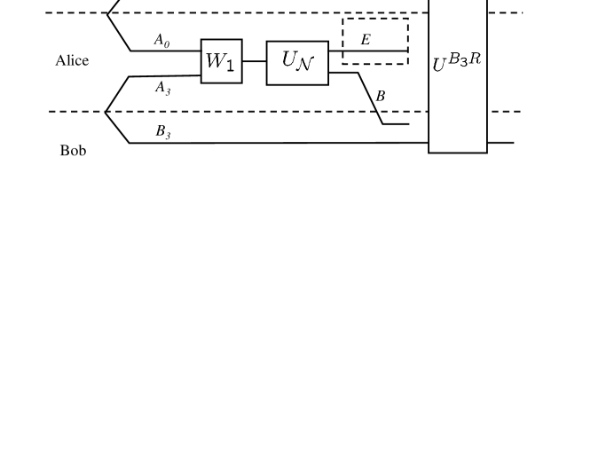
Figure 3: Partial reduction from the father to the mother. Dotted lines are used to demarcate domains controlled by the different partipicants and solid lines represent quantum information. Note that Alice starts the protocol sharing one maximally entangled state with the reference, $|\Phi_{0}\rangle^{A_{0}R}$, and another with Bob, $|\Phi_{3}\rangle^{A_{3}B_{3}}$. The unitary transformation $U^{B_{3}R}$ comes from an application of the FQSW theorem with $B_{3}R$ replacing $A_{1}A_{2}$. After the application of the unitary, the registers $R$ and $E$ are nearly decoupled, as desired, but unfortunately, because it requires acting on the reference system $R$, $U^{B_{3}R}$ cannot be used in this way.

Thus, there exist isometries $U^{B_{3}R\rightarrow B_{3}R}$ and $V^{B_{3}B\rightarrow\widehat{B}\tilde{B}}$ such that

$$\|(V\circ U)\psi^{B_{3}RBE}(V\circ U)^{\dagger}-\psi^{\widehat{B}E}\otimes\Phi_{0}^{R\tilde{B}}\|_{1}\leq 2\!\left[\frac{2d_{B_{3}R}d_{E}}{d^{2}_{B_{3}}}\Big{\{}\!\!\operatorname{Tr}[(\psi^{B_{3}RE})^{2}]+2\operatorname{Tr}[(\psi^{B_{3}R})^{2}]\operatorname{Tr}[(\psi^{E})^{2}]\Big{\}}\right]^{1/4}\!\!\!\!,$$

where $W^{\widehat{B}\rightarrow B_{3}RB}|\psi\rangle^{\widehat{B}E}=|\psi\rangle^{B_{3}RBE}$ for some isometry $W$. In particular, let

$$|\psi\rangle^{B_{3}RBE}=U_{\cal N}^{A\rightarrow BE}\circ W_{1}^{A_{0}A_{3}\rightarrow A}(|\Phi_{0}\rangle^{RA_{0}}|\Phi_{3}\rangle^{B_{3}A_{3}})$$ (31)

for some Stinespring dilation $U_{\cal N}^{A\rightarrow BE}$ of a noisy channel ${\cal N}^{A\rightarrow BE}$, and isometry $W_{1}^{A_{0}A_{3}\rightarrow A}$. Since $V^{B_{3}B\rightarrow\widehat{B}\tilde{B}}$ acts entirely on systems held by Bob, it could be performed by him as a decoding operation. The isometry $U^{B_{3}R\rightarrow B_{3}R}$, on the other hand, acts on the reference system, which is not allowed to participate actively in the protocol. The situation up to this point is depicted in Figure 3. However, because $\Phi_{0}^{RA_{0}}\otimes\Phi_{3}^{B_{3}A_{3}}$ is maximally entangled between $A_{3}A_{0}$ and $B_{3}R$,

$$U^{B_{3}R\rightarrow B_{3}R}(|\Phi_{0}\rangle^{RA_{0}}|\Phi_{3}\rangle^{B_{3}A_{3}})=(U^{T})^{A_{3}A_{0}\rightarrow A_{3}A_{0}}(|\Phi_{0}\rangle^{RA_{0}}|\Phi_{3}\rangle^{B_{3}A_{3}}),$$

where $T$ denotes transposition. Thus, the effect of $U$ can be achieved by acting instead with $U^{T}$ on $A_{3}A_{0}$, systems held by Alice. Defining $W_{2}^{A_{0}A_{3}\rightarrow A}=W_{1}\circ U^{T}$, we get

$$\begin{split}&\|(V\circ U_{\cal N}\circ W_{2})(\Phi_{0}^{RA_{0}}\otimes\Phi_{3}^{B_{3}A_{3}})(V\circ U_{\cal N}\circ W_{2})^{\dagger}-\psi^{\widehat{B}E}\otimes\Phi_{0}^{R\tilde{B}}\|_{1}\\ &\phantom{=====}\leq 2\left[\frac{2d_{A_{0}A_{3}}d_{E}}{d^{2}_{A_{3}}}\Big{\{}\operatorname{Tr}[(\psi^{B})^{2}]+\frac{2}{d_{A_{0}A_{3}}}\operatorname{Tr}[(\psi^{E})^{2}]\Big{\}}\right]^{1/4}.\end{split}$$ (32)

This is precisely the setting of the father protocol, as illustrated in Figure 4.

Alice needs to transfer the purification of some maximally mixed state $\Phi_{0}^{R}$ to Bob. The resources at their disposal are the channel ${\cal N}^{A\rightarrow B}$ and a maximally entangled state $\Phi_{3}^{B_{3}A_{3}}$. Alice performs the encoding $W_{2}$, sends the resulting state through the channel ${\cal N}$ and Bob decodes with $V$. The number of ebits used up is $\log d_{A_{3}}$ whereas the number of qubits sent is $\log d_{A_{0}}$.

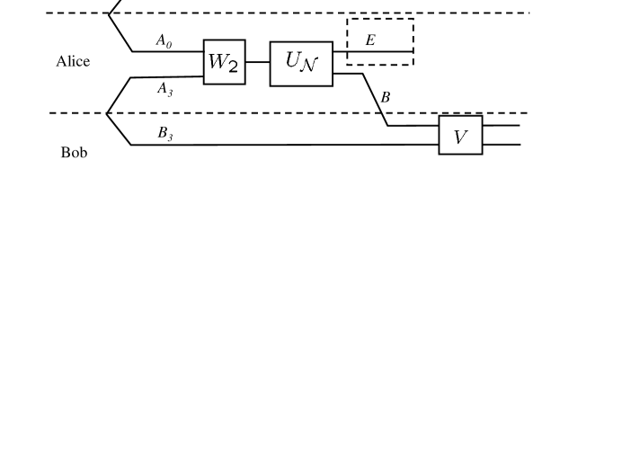
Figure 4: Final version of the father protocol generated from FQSW. As Figure 3 makes clear, $U^{B_{3}B}$ was required to act on one half of a maximally entangled state, the other half of which found in $A_{3}A_{0}$, register held by Alice. Thus, Alice can instead implement the encoding operation $W_{2}=W_{1}\circ U^{T}$. Bob performs the decoding operation $V$ mandated by FQSW, resulting in the one-shot father.

VI Fully quantum reverse Shannon theorem: one-shot version

The quantum reverse Shannon theorem was conceived of in BSST99 ; BSST02 , and is proved in full in BDHSW06 . It asserts that in the presence of entanglement, a noisy quantum channel ${\cal N}$ can be simulated by $C_{E}({\cal N})$ cbits of forward classical communication per copy of the channel, where $C_{E}$ is the entanglement-assisted capacity of the channel.

Here, following D05b , we demonstrate how, by running the mother protocol backwards, one obtains a simple proof of a fully quantum version of this result. The Stinespring dilation $U_{{\cal N}}\mathrel{\mathop{\mathchar 58\relax}}A^{\prime}\rightarrow BE$ of ${\cal N}^{A^{\prime}\rightarrow B}$ is simulated in such a way that $E$ ends up with Alice. For that reason, we say that the protocol simulates the feedback channel associated to ${\cal N}^{A^{\prime}\rightarrow B}$.

Ultimately, in section IX, we will show the fully quantum reverse Shannon (FQRS) resource inequality

$$\frac{1}{2}I(A;B)_{\varphi}[q\rightarrow q]+\frac{1}{2}I(B;E)_{\varphi}[qq]\geq\left\langle U_{{\cal N}}^{A^{\prime}\rightarrow BE}\mathrel{\mathop{\mathchar 58\relax}}\rho^{A^{\prime}}\right\rangle,$$ (33)

where $|\varphi\rangle^{ABE}=U_{{\cal N}}^{A^{\prime}\rightarrow BE}|\varphi\rangle^{AA^{\prime}}$ and $|\varphi\rangle^{AA^{\prime}}$ is a purification of $\rho^{A^{\prime}}$. In this section, we will actually prove a one-shot version of this resource inequality, by a simple re-interpretation of the systems of the mother, and running her backwards in time. The task is to simulate with high fidelity the feedback channel $U_{{\cal N}}\mathrel{\mathop{\mathchar 58\relax}}A^{\prime}\rightarrow BE$ on a source ${\psi}^{AA^{\prime}}$, using some maximal entanglement $\Phi^{\tilde{A}\tilde{B}}$ and quantum communication of a system $A_{1}$ of dimension $d_{A_{1}}$. From a mathematical point of view, the state $|\psi\rangle^{ABE}=U_{{\cal N}}^{A^{\prime}\rightarrow BE}|\psi\rangle^{AA^{\prime}}$ has to be created from $|\psi\rangle^{AA^{\prime}}\otimes|\Phi\rangle^{\tilde{A}\tilde{B}}$, as illustrated in Figure 5.

Recall that the one-shot FQSW protocol created a product state starting from an arbitrary pure tripartite entangled state, whereas here the goal is to do the reverse. Hence the need to run the protocol backwards in time. To help see the appropriate choice of relabellings, note that in the FQSW case, Bob holds purifications of the $R$ and $A_{2}$ systems, called $\widehat{B}$ and $\tilde{B}$ respectively. In the present setting, Alice starts holding purifications $A^{\prime}$ and $\tilde{A}$ of $A$ and $\tilde{B}$ respectively. Matching the corresponding systems suggests the following replacements in the one-shot mother:

FQRS	FQSW
$A^{\prime}$	$\widehat{B}$
$A$	$R$
$B$	$A$
$E$	$B$
$\tilde{A}$	$\tilde{B}$
$\tilde{B}$	$A_{2}$

Figure 5: a) The starting point for FQRS, a pair of pure entangled states. The system $A$ is a purification of Alice’s input system $A^{\prime}$ while $\tilde{A}\tilde{B}$ holds the entanglement that Alice-Bob will consume to execute the protocol. b) After execution of the protocol, the reference system $A$ is unchanged while Alice receives the environment feedback system $E$ and Bob receives his share $B$ of the state $|\psi\rangle^{ABE}=U_{{\cal N}}^{A^{\prime}\rightarrow BE}|\psi\rangle^{AA^{\prime}}$.

A comparison of Figure 5 with the FQRS analogue, Figure 1 is also very helpful for clarifying the role of the substitutions. We can interpret theorem IV.1 as saying that there exist isometries $U^{B\rightarrow A_{1}\tilde{B}}$ and $V^{A_{1}E\rightarrow A^{\prime}\tilde{A}}$ such that

$$\begin{split}\bigl{\|}\psi^{ABE}-(U^{\dagger}\circ V^{\dagger})(\psi^{AA^{\prime}}\otimes\Phi^{\tilde{A}\tilde{B}})(U^{\dagger}\circ V^{\dagger})^{\dagger}\bigr{\|}_{1}&=\|(V\circ U)\psi^{ABE}(V\circ U)^{\dagger}-\psi^{AA^{\prime}}\otimes\Phi^{\tilde{A}\tilde{B}}\|_{1}\\ &\!\!\!\!\!\!\!\!\!\leq 2\!\left[\frac{2d_{B}d_{A}}{d^{2}_{A_{1}}}\Big{\{}\operatorname{Tr}[(\psi^{AB})^{2}]+2\operatorname{Tr}[(\psi^{A})^{2}]\operatorname{Tr}[(\psi^{B})^{2}]\Big{\}}\right]^{1/4}\!\!.\end{split}$$

In other words, Alice performs $V^{\dagger}\mathrel{\mathop{\mathchar 58\relax}}A^{\prime}\tilde{A}\rightarrow A_{1}E$ on her part of the system, and sends $A_{1}$ to Bob; she keeps $E$ which will be the environment of the channel. (Note that because of the input state, $V^{\dagger}$ is actually a well-defined isometry!) Bob can perform the isometry $U^{\dagger}\mathrel{\mathop{\mathchar 58\relax}}A_{1}\tilde{B}\rightarrow B$ to obtain the channel output in $B$.

VII Fully quantum Slepian-Wolf: i.i.d. version

We return now to the setting where Alice, Bob and the reference system share the state $|\psi^{\prime}\rangle=(|\varphi\rangle^{ABR})^{\otimes n}$. This is often called the i.i.d. case because each copy of the state is identical and independently distributed. Combining the one-shot, fully quantum Slepian-Wolf result with Schumacher compression will lead to the FQSW resource inequality (2). In Appendix A we show the following: For any $\epsilon,\delta>0$ and sufficiently large $n$, we can define projectors $\Pi_{A},\Pi_{B},\Pi_{R}$ onto the $\delta$-typical subspaces of the systems indicated by the subscripts such that the following properties hold for any subsystem $F=A,B,R$:

1. $\|{\cal E}(\psi^{\prime})-\psi^{\prime}\|_{1}\leq\epsilon$,

2. $\|\psi-\psi^{\prime}\|_{1}\leq\epsilon$,

3. $2^{n[H(F)-\delta]}\leq\operatorname{rank}\Pi_{F}\leq 2^{n[H(F)+\delta]}$,

4. $\operatorname{Tr}[(\psi^{F})^{2}]\leq 2^{-n[H(F)-\delta]}$.

Here ${\cal E}^{A\rightarrow A^{typ}}$ is the Schumacher compression operation (one of whose Kraus elements is $\Pi_{A}$) and $|\psi\rangle$ the normalized version of the state

$$(\Pi_{A}\otimes\Pi_{B}\otimes\Pi_{R})|\psi^{\prime}\rangle.$$ (34)

While we are concerned with the output of the protocol when it is applied to the state $|\psi^{\prime}\rangle=(|\varphi\rangle^{ABR})^{\otimes n}$, by properties i) and ii) we can analyze its effect on the nearly indistinguishable $|\psi\rangle$ instead.

Thanks to the properties of the typical projectors, namely properties iii) and iv), the various quantities appearing in the upper bound of Theorem IV.2 get replaced by entropic formulas in the i.i.d. case. For an arbitrary subsystem $F$, let $F^{typ}$ denote the support of $\Pi_{F}$ and assume $A^{typ}=A_{1}\otimes A_{2}$. By Theorem IV.1, there exist isometries $U^{A^{typ}\rightarrow A_{1}A_{2}}$ and $V^{A_{1}B\rightarrow\widehat{B}\tilde{B}}$ such that

$$\begin{split}&\big{\|}(V\circ U)\psi^{R^{typ}A^{typ}B}(V\circ U)^{\dagger}-\psi^{R^{typ}\widehat{B}}\otimes\Phi^{A_{2}\tilde{B}}\big{\|}_{1}\\ &\phantom{====}\leq 2\left[\frac{2d_{A^{typ}}d_{R^{typ}}}{d^{2}_{A_{1}}}\Big{\{}\operatorname{Tr}[(\psi^{A^{typ}R^{typ}})^{2}]+2\operatorname{Tr}[(\psi^{A^{typ}})^{2}]\operatorname{Tr}[(\psi^{R^{typ}})^{2}]\Big{\}}\right]^{1/4}\\ &\phantom{====}\leq 2(4\cdot 2^{n[I(A;R)+3\delta]}/d^{2}_{A_{1}})^{1/4}.\end{split}$$ (35)

Choosing $\log d_{A_{1}}=n[I(A;R)/2+2\delta]$, the bound of Eq. (35) becomes less than or equal to $\sqrt{8}2^{-n\delta/4}$.

Since $\psi$, ${\cal E}(\psi^{\prime})$ and $\psi^{\prime}$ are close, performing the protocol on the Schumacher compressed state ${\cal E}(\psi^{\prime})$ will also do well. More precisely, a double application of the triangle inequality and properties i) and ii) give

$$\|(V\circ U){\cal E}({\psi^{\prime}}^{RAB})(V\circ U)^{\dagger}-{\psi^{\prime}}^{R\widehat{B}}\otimes\Phi^{A_{2}\tilde{B}}\|_{1}\leq 2\epsilon+\sqrt{8}2^{-n\delta/4}.$$

The number of qubit channels used up is thus $n[I(A;R)/2+2\delta]$, whereas the number of ebits distilled is $\log d_{A_{2}}=\log d_{A^{typ}}-\log d_{A_{1}}\geq n[I(A;B)/2-3\delta]$.

VIII Father: i.i.d. version

In the i.i.d. father setting described by the resource inequality (4), Alice and Bob are given a channel of the form $({\cal N}^{A^{\prime}\rightarrow B})^{\otimes n}$. Choose a Stinespring dilation ${U_{\cal N}}^{A^{\prime}\rightarrow BE}$ such that ${\cal N}(\rho)=\operatorname{Tr}_{E}U\rho U^{\dagger}$ and define $|\varphi\rangle^{ABE}={U_{\cal N}}|\varphi\rangle^{AA^{\prime}}$. Let $|\psi\rangle$ and $|\psi^{\prime}\rangle$ be as in the previous section, only with $R$ replaced by $E$. Now define $\Pi^{t}_{A}$ to be the projector onto a particular typical type $t$ and define $|\psi_{t}^{\prime}\rangle$ and $|\psi_{t}\rangle$ to be the normalized versions of the states ${\Pi^{t}_{A}|\psi^{\prime}\rangle}$ and $\Pi^{t}_{A}|\psi\rangle$, respectively. In Appendix A it is shown that there exists a particular $\Pi^{t}_{A}$ such that the following properties hold:

1. $\psi_{t}^{A}=I/(\operatorname{rank}\Pi^{t}_{A})$ ,

2. $\|\psi_{t}-\psi_{t}^{\prime}\|_{1}\leq\epsilon$,

3. $2^{n[H(F)-\delta]}\leq\operatorname{rank}\Pi_{F}\leq 2^{n[H(F)+\delta]}$,

4. $\operatorname{Tr}[(\psi_{t}^{F})^{2}]\leq 2^{-n[H(F)-\delta]}$.

5. $2^{n[H(A)-\delta]}\leq\operatorname{rank}\Pi^{t}_{A}\leq 2^{n[H(A)+\delta]}$

Let $A_{t}$ denote the support of $\Pi^{t}_{A}$. By property i), $|\psi^{\prime}_{t}\rangle^{A_{t}BE}$ is the result of sending a maximally entangled state proportional to $|\Phi\rangle^{A_{t}A^{\prime}_{t}}=(\Pi_{t}^{A}\otimes\Pi_{t}^{A^{\prime}})(|\varphi\rangle^{AA^{\prime}})^{\otimes n}$ through ${U_{\cal N}}^{\otimes n}$. Similarly, $|\psi_{t}\rangle^{A_{t}B^{typ}E^{typ}}$ arises from the modified channel $(\Pi_{B}\otimes\Pi_{E})\circ{U_{\cal N}}^{\otimes n}$. Thus $|\psi_{t}\rangle^{A_{t}BE}$ is of the form $(\ref{partic})$, and we can apply the results of section V. Proceeding as in the previous section and using the above properties we conclude that there exist isometries $W_{2}^{A_{0}A_{3}\rightarrow A}$ and $V^{B_{3}B\rightarrow\widehat{B}\tilde{B}}$ such that

$$\|(V\circ U_{\cal N}^{\otimes n}\circ W_{2})(\Phi_{0}^{RA_{0}}\otimes\Phi_{3}^{B_{3}A_{3}})(V\circ U_{\cal N}^{\otimes n}\circ W_{2})^{\dagger}-\psi_{t}^{\widehat{B}E}\otimes\Phi_{0}^{R\tilde{B}}\|_{1}\\ \leq 2\epsilon+\sqrt{8}2^{-n\delta/4}.$$

The number of ebits used up is $\log d_{A_{3}}=n[I(A;E)/2+2\delta]$ and the number of qubits transmitted is $\log d_{A_{0}}=\log d_{A_{t}}-\log d_{A_{3}}\geq n[I(A;B)/2-3\delta]$, leading to the asymptotic rates required by the father resource inequality.

IX Fully quantum reverse Shannon theorem: i.i.d. version

As in the previous two sections, we can consider the special case in which Alice and Bob want to simulate many realizations of the channel ${\cal N}\mathrel{\mathop{\mathchar 58\relax}}A\rightarrow B$, or rather its feedback isometry $U_{{\cal N}}\mathrel{\mathop{\mathchar 58\relax}}A\rightarrow BE$, relative to a source $\rho^{A}$. The FQRS resource inequality (33) was described in section VI. Just as in section VII, the resource inequality is achieved by mentally truncating the state $\bigl{(}|\varphi\rangle^{ABE}\bigr{)}^{\otimes n}$ to its typical part, introducing small disturbances, and then running the one-shot protocol on the truncated state. We omit the details.

X Correlated source coding: distributed compression

One of the major applications of the state merging inequality (3) is to the problem of distributed compression with free forward (or indeed completely unrestricted) classical communication. For this problem, Horodecki, Oppenheim and Winter demonstrated that the resulting region of achievable rates has the same form as the classical Slepian-Wolf problem SW71 ; HOW05 . In this section, we consider the application of the fully quantum Slepian-Wolf inequality to distributed compression without classical communication.

Because distributed compression studies multiple senders, it no longer fits into the resource inequality framework as laid out in DHW05 . We therefore begin with some definitions describing the task to be performed. A source provides Alice and Bob with the $A$ and $B$ parts of a quantum state $|\psi\rangle=(|\varphi\rangle^{ABR})^{\otimes n}$ purified by a reference system $R$. They must independently compress their shares and transmit them to a receiver Charlie. That is, they will perform encoding operations $E_{A}$ and $E_{B}$ described by completely positive, trace-preserving (CPTP) maps with outputs on systems $C_{A}$ and $C_{B}$ of dimensions $2^{nQ_{A}}$ and $2^{nQ_{B}}$, respectively. The receiver, Charlie, will then perform a decoding operation, again described by a CPTP map, this time with output systems $\widehat{A}$ and $\widehat{B}$ isomorphic to $A^{n}$ and $B^{n}$. A rate pair $(Q_{A},Q_{B})$ will be said to be achievable if for all $\epsilon>0$ there exists an $N(\epsilon)>0$, such that for all $n\geq N(\epsilon)$ there exists a corresponding $(E_{A},E_{B},D)$ such that

$$\langle\psi|^{R^{n}\widehat{A}\widehat{B}}(D\circ(E_{A}\otimes E_{B}))(\psi^{R^{n}A^{n}B^{n}})|\psi\rangle^{R^{n}\widehat{A}\widehat{B}}\geq 1-\epsilon.$$ (36)

The achievable rate region ${\cal S}{\cal W}(\varphi)$ for a given $|\varphi\rangle$ is the closure of the set of achievable rates. By time-sharing it is a convex set.

The fully quantum Slepian-Wolf inequality provides a natural class of protocols for this task. One party, say Bob, first Schumacher compresses his share and sends it to Charlie. This is possible provided $Q_{B}>H(B)_{\varphi}$. The other party, in this case Alice, then implements the fully quantum Slepian-Wolf protocol with Charlie playing the role of Bob. This is possible provided $Q_{A}>I(A;R)/2$. Looking at the total number of qubits required gives a curious symmetrical formula:

$$Q_{A}+Q_{B}>\frac{1}{2}I(A;R)_{\varphi}+H(B)_{\varphi}=\frac{H(A)_{\varphi}+H(B)_{\varphi}+H(AB)_{\varphi}}{2}=\mathrel{\mathop{\mathchar 58\relax}}\frac{1}{2}J(A;B)_{\varphi},$$ (37)

introducing a new symbol $J(A;B)=H(A)+H(B)+H(AB)$ for the characteristic rate sum above, a kind of quasi-mutual information with a plus sign instead of minus.

By switching the roles played by Alice and Bob and also time-sharing between the resulting two protocols, we find

Theorem X.1

The region defined by

$$Q_{A} \geq\frac{1}{2}I(A;R)_{\varphi}$$

$$Q_{B} \geq\frac{1}{2}I(B;R)_{\varphi}$$ (38)

$$Q_{A}+Q_{B} \geq\frac{1}{2}J(A;B)_{\varphi}$$

is contained in the achievable rate region ${\cal S}{\cal W}(\varphi)$.     $\sqcap$$\sqcup$

In fact, the region of Theorem X.1 is in some cases equal to ${\cal S}{\cal W}(\varphi)$, as we will see by proving a general outer bound on the achievable rate region. Assume that $(Q_{A},Q_{B})\in{\cal S}{\cal W}(\varphi)$. To begin, fix $n>N(\epsilon)$ and let $W_{A}$ and $W_{B}$ be the environments for the Stinespring dilations of the encoding operations $E_{A}$ and $E_{B}$. We may without loss of generality assume that their dimensions $d_{W_{A}}$, $d_{W_{B}}$ are bounded above by $d_{A}^{2n}$, $d_{B}^{2n}$, respectively, because every CPTP map from a space of dimension $d$ to a space of dimension at most $d$ can be written using at most $d^{2}$ Kraus operators.

To bound $Q_{A}$, assume that Charlie has received both $C_{B}$ and $W_{B}$, that is, all of $B^{n}$. Let $W_{C}$ be the environment for the dilation of Charlie’s $D$. Again, without loss of generality we can assume that the Stinespring dilations are implemented by preparing the environment systems in pure unentangled states and then applying unitary transformations. Because at the end of the protocol Charlie must have essentially $A^{n}B^{n}$, which purifies $R^{n}$, the registers $W_{A}W_{C}$ have to be in a pure state of their own, product with $R^{n}$ and Charlie’s output $\widehat{A}\widehat{B}$. Of course, this is not exactly true, only with high fidelity, so we proceed to make these statements rigorous.

Let $|\xi\rangle^{R^{n}\widehat{A}\widehat{B}W_{A}W_{C}}$ be the final state after the application of the Stinespring dilations of the encoding and decoding. By the fidelity condition,

$$\lambda_{\operatorname{max}}(\xi^{R^{n}\widehat{A}\widehat{B}})\geq\operatorname{Tr}\bigl{[}\xi^{R^{n}\widehat{A}\widehat{B}}|\psi\rangle\!\langle\psi|^{R^{n}\widehat{A}\widehat{B}}\bigr{]}\geq 1-\epsilon,$$

where $\lambda_{\operatorname{max}}(\xi^{R^{n}\widehat{A}\widehat{B}})$ denotes the maximum eigenvalue of $\xi^{R^{n}\widehat{A}\widehat{B}}$. Therefore, $|\xi\rangle^{R^{n}\widehat{A}\widehat{B}W_{A}W_{C}}$ has Schmidt decomposition

$$|\xi\rangle^{R^{n}\widehat{A}\widehat{B}W_{A}W_{C}}=\sum_{i}\sqrt{\lambda_{i}}|v_{i}\rangle^{R^{n}\widehat{A}\widehat{B}}|w_{i}\rangle^{W_{A}W_{C}},$$ (39)

where $\lambda_{1}=\lambda_{\operatorname{max}}\geq 1-\epsilon$, and consequently,

$$\operatorname{Tr}\bigl{[}|\xi\rangle\!\langle\xi|^{R_{n}\widehat{A}\widehat{B}W_{A}W_{C}}(\xi^{R^{n}\widehat{A}\widehat{B}}\otimes\xi^{W_{A}W_{C}})\bigr{]}\geq\sqrt{1-\epsilon}^{2}(1-\epsilon)^{2}\geq 1-3\epsilon.$$

So, since the above is the fidelity between states,

$$\left\||\xi\rangle^{R^{n}\widehat{A}\widehat{B}W_{A}W_{C}}-\xi^{R^{n}\widehat{A}\widehat{B}}\otimes\xi^{W_{A}W_{C}}\right\|_{1}\leq 2\sqrt{3\epsilon},$$

by FvG99 , and with the contractivity of the trace distance we now have

$$\left\|\xi^{R^{n}W_{A}}-\xi^{R^{n}}\otimes\xi^{W_{A}}\right\|_{1}\leq 2\sqrt{3\epsilon},$$ (40)

We can now apply the Fannes inequality F73 to yield:

$$\begin{split}\left|H(\xi^{R^{n}W_{A}})-H(\xi^{R^{n}}\otimes\xi^{W_{A}})\right|&\leq 2\sqrt{3\epsilon}\log(d_{A}^{n}d_{B}^{n}d_{W_{A}})+\eta(2\sqrt{3\epsilon})\\ &\leq 2\sqrt{3\epsilon}n\log(d_{A}^{3}d_{B})+\eta(2\sqrt{3\epsilon}),\end{split}$$ (41)

for $\epsilon\leq\frac{1}{12e^{2}}$, $\eta(x)=-x\log x$ and using $d_{W_{A}}\leq d_{A}^{2n}$.

Now, using the subadditivity of the von Neumann entropy and the fact that the overall state is pure we have

$$H(B^{n})+H(C_{A}) \geq H(B^{n}C_{A})=H(W_{C}\widehat{A}\widehat{B})=H(W_{A}R^{n})$$

$$\geq H(W_{A})+H(R^{n})-2\sqrt{3\epsilon}n\log(d_{A}^{3}d_{B})-\eta(2\sqrt{3\epsilon})$$

$$\geq H(A^{n})-H(C_{A})+H(R^{n})-2\sqrt{3\epsilon}n\log(d_{A}^{3}d_{B})-\eta(2\sqrt{3\epsilon}).$$

Therefore,

$$2nQ_{A} \geq 2H(C_{A})$$

$$\geq H(A^{n})-H(B^{n})+H(R^{n})-2\sqrt{3\epsilon}n\log(d_{A}^{3}d_{B})-\eta(2\sqrt{3\epsilon})$$

$$=nI(A;R)-2\sqrt{3\epsilon}n\log(d_{A}^{3}d_{B})-\eta(2\sqrt{3\epsilon})$$

Dividing by $n$ and letting $\epsilon\rightarrow 0$, we obtain

$$Q_{A}\geq\frac{1}{2}I(A;R).$$ (42)

Switching the roles of Alice and Bob gives the corresponding inequality,

$$Q_{B}\geq\frac{1}{2}I(B;R).$$ (43)

To bound $Q_{A}+Q_{B}$ let us return to the situation where Alive and Bob perform their original encoding. Then,

$$H(A^{n})=H(C_{A}W_{A})\leq H(W_{A})+H(C_{A})\leq H(W_{A})+nQ_{A}.$$ (44)

The first equality follows from the fact that the environment system is initiated as a pure unentangled state and from the unitary invariance of the von Neumann entropy.

Combining with the analogous inequality for $B$ leads to,

$$n(Q_{A}+Q_{B})\geq n[H(A)+H(B)]-H(W_{A})-H(W_{B}).$$ (45)

By similar arguments as before,

$$|H(W_{A}W_{B}R^{n})-H(W_{A}W_{B})-H(R^{n})|\leq 2\sqrt{3\epsilon}n\log(d_{A}^{2}d_{B}^{2}d_{R})+\eta(2\sqrt{3\epsilon}),$$ (46)

for $\epsilon$ small enough. So,

$$\begin{split}H(C_{A}C_{B})&=H(W_{A}W_{B}R^{n})\\ &\geq H(W_{A})+H(W_{B})-I(W_{A};W_{B})+H(R^{n})\\ &\phantom{==}-2\sqrt{3\epsilon}n\log(d_{A}^{2}d_{B}^{2}d_{R})-\eta(2\sqrt{3\epsilon}).\end{split}$$

Using the purity of the overall state, however, gives $H(R^{n})=nH(AB)$, which combined with the bound $H(C_{A}C_{B})\leq n(Q_{A}+Q_{B})$, leads to the inequality

$$\begin{split}H(W_{A})+H(W_{B})&\leq n(Q_{A}+Q_{B})-nH(AB)+I(W_{A};W_{B})\\ &+2\sqrt{3\epsilon}n\log(d_{A}^{2}d_{B}^{2}d_{R})+\eta(2\sqrt{3\epsilon})\end{split}$$ (47)

Adding equations (45) and (47),

$$\begin{split}2n(Q_{A}+Q_{B})&\geq n\bigl{(}H(A)+H(B)+H(AB)\bigr{)}-I(W_{A};W_{B})\\ &\phantom{==}-n\sqrt{3}\epsilon\log(d_{A}^{2}d_{B}^{2}d_{R})-\eta(\sqrt{3}\epsilon).\end{split}$$ (48)

Thus,

$$Q_{A}+Q_{B}\geq\frac{1}{2}J(A;B)-\frac{1}{n}I(W_{A};W_{B})-2\sqrt{3\epsilon}\log(d_{A}^{2}d_{B}^{2}d_{R})-\frac{\eta(2\sqrt{3\epsilon})}{n}$$ (49)

Now, let $T\mathrel{\mathop{\mathchar 58\relax}}R^{n}\to R^{\prime}$ be any CPTP map on $R^{n}$. Then we can bound the mutual information $I(W_{A};W_{B})$ as follows.

$$\begin{split}I(W_{A};W_{B})-I(W_{A};W_{B}|R^{\prime})&=\bigl{(}H(W_{A})-H(W_{A}R^{\prime})\bigr{)}+\bigl{(}H(W_{B})-H(W_{B}R^{\prime})\bigr{)}\\ &\phantom{==}-\bigl{(}H(W_{A}W_{B})-H(W_{A}W_{B}R^{\prime})\bigr{)}-H(R^{\prime})\\ &\leq 8\sqrt{3\epsilon}\bigl{(}\log d_{W_{A}}+\log d_{W_{B}}+\log d_{W_{A}}d_{W_{B}}\bigr{)}+6H_{2}(2\sqrt{3\epsilon})\\ &\leq 8\sqrt{3\epsilon}n\log(d_{A}^{4}d_{B}^{4})+6H_{2}(2\sqrt{3\epsilon}),\end{split}$$

where we have used that $W_{A}W_{B}$ is almost uncorrelated with $R^{\prime}$ (via the contractivity of the trace distance under CPTP maps):

$$\|\xi^{W_{A}W_{B}R^{\prime}}-\xi^{W_{A}W_{B}}\otimes\xi^{R^{\prime}}\|_{1}\leq 2\sqrt{3\epsilon},$$

followed by the Alicki-Fannes inequality AF04 . The function $H_{2}(x)$ is the binary entropy $H_{2}(x)=-x\log x-(1-x)\log(1-x)$. Note that in this way the dimension of $R^{\prime}$ doesn’t enter, which is desirable as we do not wish to constrain it in any way.

In particular, for small $\epsilon$,

$$\begin{split}I(W_{A};W_{B})&\leq I(W_{A};W_{B}|R^{\prime})+8\sqrt{3\epsilon}n\log(d_{A}^{4}d_{B}^{4})+6H_{2}(2\sqrt{3\epsilon})\\ &\leq I(A^{n};B^{n}|R^{\prime})+8\sqrt{3\epsilon}n\log(d_{A}^{4}d_{B}^{4})+6H_{2}(2\sqrt{3\epsilon})\end{split}$$ (50)

where in the second line we have invoked the monotonicity of mutual information under local operations. Therefore,

$$\begin{split}Q_{A}+Q_{B}&\geq\frac{1}{2}J(A;B)-\frac{1}{2n}I(A^{n};B^{n}|R^{\prime})\\ &\phantom{==}-2\sqrt{3\epsilon}\log(d_{A}^{2}d_{B}^{2}d_{R})-\frac{\eta(2\sqrt{3\epsilon})}{n}-8\sqrt{3\epsilon}\log(d_{A}^{4}d_{B}^{4})-\frac{6H_{2}(2\sqrt{3\epsilon})}{n}\end{split}$$

By optimising over the CPTP map $T$, we thus obtain

$$\begin{split}Q_{A}+Q_{B}&\geq\frac{1}{2}J(A;B)-\frac{1}{n}E_{\rm sq}\bigl{(}(\varphi^{AB})^{\otimes n}\bigr{)}-10\sqrt{3\epsilon}\log(d_{A}^{4}d_{B}^{4})-\frac{7H_{2}(2\sqrt{3\epsilon})}{n}\\ &=\frac{1}{2}J(A;B)-E_{\rm sq}(\varphi^{AB})-10\sqrt{3\epsilon}\log(d_{A}^{4}d_{B}^{4})-\frac{7H_{2}(2\sqrt{3\epsilon})}{n},\end{split}$$

where $E_{\rm sq}(\varphi^{AB})$ is the squashed entanglement of $\varphi^{AB}$, defined as the infimum of $\mbox{$\frac{1}{2}$}I(A;B|E)$ over extensions $\varphi^{ABE}$ of $\varphi^{AB}$ CW04 . We have used explicitly the fact, proved in the cited paper, that $E_{\rm sq}(\varphi^{\otimes n})=nE_{\rm sq}(\varphi)$.

Since $\epsilon>0$ was arbitrary, we have therefore proved the following outer bound on the achievable rate region:

Theorem X.2

The rate region ${\cal S}{\cal W}(\varphi)$ of fully quantum distributed compression of the source $\varphi$ is contained in the set defined by the inequalities

$$Q_{A} \geq\frac{1}{2}I(A;R)_{\varphi}$$

$$Q_{B} \geq\frac{1}{2}I(B;R)_{\varphi}$$ (51)

$$Q_{A}+Q_{B} \geq\frac{1}{2}J(A;B)_{\varphi}-E_{\rm sq}(\varphi^{AB}).\qquad\hbox{\hbox to0.0pt{$\sqcap$\hss}$\sqcup$}$$

In the special case where $\varphi^{AB}$ is separable, $E_{\rm sq}(\varphi)=0$, which implies that the region defined by Eq. (X.1) is optimal. Under certain further technical assumptions, namely that $\varphi^{AB}$ be the density operator of an ensemble of product pure states satisfying a condition called irreducibility, the same conclusion was found in ADHW04 . That paper, however, was unable to show that the bound was achievable.

The appearance of the squashed entanglement in (X.2) may seem somewhat mysterious, but a slight modification of the protocols based on fully quantum Slepian-Wolf will lead to an inner bound on the achievable region that is of a similar form. Specifically, let $D_{0}(\varphi^{AB})$ be the amount of pure state entanglement that Alice and Bob can distill from $\varphi^{AB}$ without engaging in any communication. Since this pure state entanglement is decoupled from the reference system $R$, they could actually perform this distillation process and discard the resulting entanglement before beginning one of their FQSW-based compression protocols. While neither $I(A;R)$ nor $I(B;R)$ would change, each of $H(A)$ and $H(B)$ would decrease by $D_{0}(\varphi^{AB})$. The corresponding inner bound on the achievable rate region ${\cal S}{\cal W}(\varphi)$ would therefore be defined by the inequalities

$$Q_{A} \geq\frac{1}{2}I(A;R)_{\varphi}$$

$$Q_{B} \geq\frac{1}{2}I(B;R)_{\varphi}$$ (52)

$$Q_{A}+Q_{B} \geq\frac{1}{2}J(A;B)_{\varphi}-D_{0}(\varphi^{AB}).$$

The only gap between the inner and outer bounds, therefore, is a gap between different measures of entanglement.

We close this section by exhibiting a class of example sources for which we believe that the above inner bound is not tight. It is based on the observation that to arrive at (X) we considered a case where the structure of $W_{C}$ was very simple. While in principle $W_{C}$ could harbor arbitrary tripartite entanglement with $W_{A}$ and $W_{B}$, the decoding for (X), which is just the FQSW protocol’s decoding, is simply an isometry separating the entanglement with $R^{n}$ from that with one, and only one, of $W_{A}$ and $W_{B}$. Hence, we are motivated to try and construct a source that permits Alice and Bob to extract and discard some “waste”, such that later on Charlie can finish off by discarding exactly the purification of that waste. The purified source is one of the twisted states HHHO05 of the form

$$|\varphi\rangle^{RA^{\prime}A^{\prime\prime}B^{\prime}B^{\prime\prime}}=\sum_{i=1}^{d}\sqrt{p_{i}}|i\rangle^{A^{\prime}}|i\rangle^{B^{\prime}}(U_{i}^{A^{\prime\prime}B^{\prime\prime}}\otimes I^{R})|\phi_{0}\rangle^{RA^{\prime\prime}B^{\prime\prime}},$$

arbitrary unitaries $U_{i}$ on the joint system $A^{\prime\prime}B^{\prime\prime}$. (It is understood that $A=A^{\prime}A^{\prime\prime}$ and $B=B^{\prime}B^{\prime\prime}$.)

Now let us assume that the reduced states $\tau_{i}^{A^{\prime\prime}B^{\prime\prime}}=U_{i}\phi_{0}^{A^{\prime\prime}B^{\prime\prime}}U_{i}^{\dagger}$ are mutually orthogonal for $i=1,\ldots,d$. Furthermore, we restrict to the case of non-local unitaries $U_{i}$, i.e. $U_{i}$ is not a tensor product of local unitaries. We conjecture that $D_{0}(\varphi^{AB})=0$ or, more specifically, that because of the nonlocal “twist”, Alice and Bob cannot extract pure states from $\varphi^{AB}$ by local operations alone. This would mean that our inner bound yields an achievable rate sum of

$$R_{A}+R_{B}=\frac{1}{2}J(A;B)=H(A)+\frac{1}{2}I(B;R).$$

However, a better rate sum is attainable because neither Alice nor Bob need to send the $A^{\prime}$, $B^{\prime}$ registers, respectively: if $A^{\prime\prime}$ and $B^{\prime\prime}$ are transmitted faithfully, Charlie can coherently measure $i$, use it to undo $U_{i}$, so that he is left with the state $\phi_{0}^{CR}$. He then has $|i\rangle$ in his waste register $W_{C}$, entangled only with the contents of Alice’s and Bob’s waste registers $W_{A}=A^{\prime}$ and $W_{B}=B^{\prime}$. He finishes off by discarding the waste register, creating $\sum_{i}\sqrt{p_{i}}|i\rangle|i\rangle$ afresh and using a controlled unitary to put back the twist $U_{i}$ onto $\phi_{0}$. Instead of the rates

$$R_{A}=H(A)=H(A^{\prime\prime})+H(A^{\prime}|A^{\prime\prime}),\quad R_{B}=\frac{1}{2}I(B;R),$$

they now use strictly less qubit resources,

$$R_{A}^{\prime}=H(A^{\prime\prime})<H(A),\quad R_{B}^{\prime}=\frac{1}{2}I(B^{\prime\prime};R)\leq\frac{1}{2}I(B;R).$$

XI On encoding complexity

While the protocols described so far make use of a unitary transformation drawn at random according to the Haar measure, that is not essential. In fact, the only place the Haar measure was used was in the proof of Lemma IV.3. Therefore, the full unitary group could be replaced by any subset yielding the same average as in the lemma. (We thank Debbie Leung for alerting us to this possibility.) In fact, DiVincenzo, Leung and Terhal have shown that

$$\int_{{{\mathbb{U}}}({{\mathbb{C}}}^{2^{n}})}(U\otimes U)X(U^{\dagger}\otimes U^{\dagger})\,dU=\frac{1}{|G_{n}|}\sum_{g\in G_{n}}(g\otimes g)X(g^{\dagger}\otimes g^{\dagger}),$$ (53)

where $G_{n}$ is the Clifford group on $n$ qubits DLT02 . They also demonstrate in that paper that choosing an element of $G_{n}$ from the uniform distribution can be done in time polynomial in $n$. More specifically, they show that a random walk on a particular set of generators for $G_{n}$ mixes in $O(n^{8})$ time, leading to an associated quantum circuit for the selected element that is of size $O(n^{2})$ gates.

Since the Schumacher compression portion of the fully quantum Slepian-Wolf protocol can also be done in polynomial time CD96 , we conclude that the encoding portion of the mother can be done efficiently. Since her immediate children, including entanglement distillation and state merging, are built by composing the mother with efficient protocols, namely superdense coding and teleportation, their encodings can also be found and implemented efficiently.

The transformation from FQSW to the father, however, included another non-constructive step, namely the choice of a good type class. Since the number of type classes is polynomial in the number of qubits in the input, however, that step could also be implemented efficiently. The corresponding isometries mapping the shared maximally entangled state and the input space into $A_{t}$ can also be performed efficiently CD96 . Finally, while the proof presented here implies that the transpose of a random Clifford group element can be used as the encoding operation, there is in fact no need for the transpose because the Clifford group is closed under transposition. Thus, the encoding for the father can be found and implemented in polynomial time, as can those of his children, entanglement-assisted classical communication and quantum communication over a noisy channel.

Finally, because the quantum reverse Shannon protocol consists of running FQSW backwards in time, there it is Bob’s decoding that can be found and implemented efficiently instead of Alice’s encoding.

XII Discussion

We have shown that simple representation-theoretic reasoning, specifically some quadratic averages, are sufficient to derive the powerful mother protocol: a fully quantum version of entanglement distillation with state merging. The mother, in proper mythical fashion, not only generates her children in the family tree but also the father protocol and his offspring, the quantum reverse Shannon theorem, plus an almost complete solution to the distributed quantum compression problem. We leave it as an open problem to determine the exact rate region, which we conjecture to be given by

$$Q_{A} \geq\frac{1}{2}I(A;R),\quad Q_{B}\geq\frac{1}{2}I(B;R),$$

$$Q_{A}+Q_{B} \geq\frac{1}{2}J(A;B)-F(\varphi_{AB}),$$

with some functional $F(\varphi_{AB})$ of the source density operator. It is tempting to speculate that $F$, as in our inner and outer bounds on the rate region, is an entanglement monotone; note that for separable and for pure states our inner and outer bounds coincide, giving $0$ and the entropy of entanglement, respectively, in agreement with the idea that $F$ should be an entanglement measure.

We also note that while we have not pursued the opportunity here, the one-shot versions of the FQSW, father and reverse Shannon theorem are natural starting points for developing versions of the theorem adapted to states or channels with some internal structure more complicated than i.i.d. It would be interesting to compare the results of such an effort with the insights of BM04 and KW05 .

We close by highlighting a peculiar feature of the FQSW protocol. Let $|\psi\rangle$ be a pure state and suppose that Alice-Bob and Alice-Rebecca both share $n$ copies of $|\psi\rangle$, so that the global pure state is $|\varphi\rangle^{\otimes n}=(|\psi\rangle^{A_{1}R}|\psi\rangle^{A_{2}B})^{\otimes n}$. This is a “trivial” situation for FQSW. Instead of using our protocol, Alice can simply transfer her entanglement with Rebecca to Bob by compressing and sending him her $A_{1}$ registers, requiring a rate of $H(A_{1})=I(A;R)/2$. Since Alice and Bob already share $H(A_{2})=I(A;B)/2$ ebits of pure state entanglement, that completes the FQSW protocol. Because of the symmetry of the situation, the roles of Rebecca and Bob could also be reversed. Thus, Alice could transfer her Bob entanglement to Rebecca by Schumacher compressing and sending $A_{2}$ to her, requiring a rate $H(A_{2})=I(A;B)/2$. It is quite clear that Alice’s system decomposes into an $A_{1}$ part, which contains her entanglement with Rebecca, and an $A_{2}$, which contains her entanglement with Bob. Note that the entanglement structure of the final state is very different in the two cases; see Figure 6.

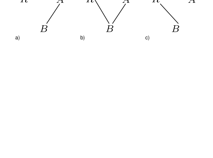
Figure 6: a) A trivial starting configuration for FQSW. Solid lines represent pure state entanglement between two parties. b) The result of Alice sending her Rebecca entanglement to Bob. c) The result of Alice sending her Bob entanglement to Rebecca.

Here’s the weirdness: if they use the general FQSW protocol instead, then since $H(A_{1})=H(A_{2})$, the same unitary will work in both case with high probability. In other words, Alice could first apply the unitary and then decide whether to transfer her Rebecca entanglement to Bob or her Bob entanglement to Eve. The only difference in Alice’s part of the protocol is whether she sends the qubits (at rate arbitrarily small above $H(A_{1})$) to Bob or to Rebecca. Thus, the localization of the entanglement so evident in the trivial implementation of the protocol disappears in the general implementation. The same subsystem can be made to carry both forms of entanglement simultaneously, compatible with either recipient!

Acknowledgments

The authors would very much like to thank Debbie Leung for bringing to their attention the possibility of replacing Haar measure unitaries with random Clifford group elements. They would also like to thank Isaac Chuang, Ignacio Cirac, Frédéric Dupuis, Renato Renner and Jürg Wullschleger for their helpful comments. AA appreciates the support of the US National Science Foundation through grant no. EIA-0086038. ID was partially supported by the NSF under grant no. CCF-0524811. PH was supported by the Canada Research Chairs program, the Canadian Institute for Advanced Research, and Canada’s NSERC. He is also grateful to the Benasque Centre for Science and CQC Cambridge for their hospitality. AW was supported by the U.K. Engineering and Physical Sciences Research Council’s “IRC QIP”, and by the EC projects RESQ (contract IST-2001-37759) and QAP (contract IST-2005-15848), as well as by a University of Bristol Research Fellowship.

Appendix A Properties of typical and type projectors.

We present here a number of consequences of the method of type classes. Denote by $x^{n}$ a sequence $x_{1}x_{2}\dots x_{n}$, where each $x_{i}$ belongs to the finite set ${\cal X}$. Denote by $|{\cal X}|$ the cardinality of ${\cal X}$. Denote by $N(x|x^{n})$ the number of occurrences of the symbol $x$ in the sequence $x^{n}$. The type $t^{x^{n}}$ of a sequence $x^{n}$ is a probability vector with elements $t^{x^{n}}_{x}=\frac{N(x_{i}|x^{n})}{n}$. Denote the set of sequences of type $t$ by

$${\cal T}^{n}_{t}=\{x^{n}\in{\cal X}^{n}\mathrel{\mathop{\mathchar 58\relax}}t^{x^{n}}=t\}.$$

For the probability distribution $p$ on the set ${\cal X}$ and $\delta>0$, let $\tau_{\delta}=\{t\mathrel{\mathop{\mathchar 58\relax}}\forall x\in{\cal X},\ |t_{x}-p_{x}|\leq\delta\}$. $|\tau_{\delta}|=a$. Define the set of $\delta$-typical sequences of length $n$ as ${\cal T}^{n}_{p,\delta}$, as

$${\cal T}^{n}_{p,\delta}=\underset{t\in\tau_{\delta}}{\bigcup}{\cal T}^{n}_{t}=\{x^{n}\mathrel{\mathop{\mathchar 58\relax}}\forall x\in{\cal X},\ |t^{x^{n}}_{x}-p_{x}|\leq\delta\}.$$ (54)

Define the probability distribution $p^{n}$ on ${\cal X}^{n}$ to be the $n$-fold product of $p$. The sequence $x^{n}$ is drawn from $p^{n}$ if and only if each letter $x_{i}$ is drawn independently from $p$. Typical sequences enjoy many useful properties CT91 ; CK81 . Let $H(p)=-\sum_{x}p_{x}\log p_{x}$ be the Shannon entropy of $p$. For any $\epsilon,\delta>0$, and all sufficiently large $n$ for which

$$p^{n}({\cal T}_{p,\delta}^{n})\geq 1-\epsilon$$ (55)

$$2^{-n[H(p)+c\delta]}\leq p^{n}(x^{n})\leq 2^{-n[H(p)-c\delta]},\,\,\,\forall x^{n}\in{\cal T}_{p,\delta}^{n}$$ (56)

$$(1-\epsilon)^{-1}2^{n[H(p)-c\delta]}\leq|{\cal T}_{p,\delta}^{n}|\leq 2^{n[H(p)+c\delta]},$$ (57)

for some constant $c$. For $t\in\tau_{\delta}$ and for sufficiently large $n$, the cardinality $D_{t}$ of ${\cal T}^{n}_{t}$ is bounded as CT91

$$D_{t}\geq 2^{n[H(p)-\iota(\delta)]}$$ (58)

and the function $\iota(\delta)\rightarrow 0$ as $\delta\rightarrow 0$.

The above concepts generalize to the quantum setting by virtue of the spectral theorem. Let $\rho=\sum_{x\in{\cal X}}p_{x}|x\rangle\langle x|$ be the spectral decomposition of a given density matrix $\rho$. In other words, $|x\rangle$ is the eigenstate of $\rho$ corresponding to eigenvalue $p_{x}$. The von Neumann entropy of the density matrix $\rho$ is

$$H(\rho)=-\operatorname{Tr}{\rho\log\rho}=H(p).$$

Define the type projector

$$\Pi^{n}_{t}=\sum_{x^{n}\in{\cal T}^{n}_{t}}|x^{n}\rangle\langle x^{n}|.$$

The typical subspace associated with the density matrix $\rho$ is defined as

$$\Pi^{n}_{\rho,\delta}=\sum_{x^{n}\in{\cal T}_{p,\delta}^{n}}|x^{n}\rangle\langle x^{n}|=\sum_{t\in\tau_{\delta}}\Pi^{n}_{t}.$$

Properties analogous to (55) – (58) hold. For any $\epsilon,\delta>0$, and all sufficiently large $n$ for which

$$\operatorname{Tr}{\rho^{\otimes n}\Pi^{n}_{\rho,\delta}}\geq 1-\epsilon$$ (59)

$$2^{-n[H(\rho)+c\delta]}\Pi^{n}_{\rho,\delta}\leq\Pi^{n}_{\rho,\delta}\rho^{\otimes n}\Pi^{n}_{\rho,\delta}\leq 2^{-n[H(\rho)-c\delta]}\Pi^{n}_{\rho,\delta},$$ (60)

$$(1-\epsilon)^{-1}2^{n[H(\rho)-c\delta]}\leq\operatorname{Tr}{\Pi^{n}_{\rho,\delta}}\leq 2^{n[H(\rho)+c\delta]},$$ (61)

for some constant $c$. For $t\in\tau_{\delta}$ and for sufficiently large $n$, the support dimension of the type projector $\Pi^{n}_{t}$ is bounded as

$$\operatorname{Tr}\Pi^{n}_{t}\geq 2^{n[H(\rho)-\iota(\delta)]}.$$ (62)

Henceforth we shall drop the $n$ and $\delta$ indices. In dealing with a multiparty system such as $|\psi^{\prime}\rangle=(|\varphi\rangle^{ABR})^{\otimes n}$, we shall label the typical projectors corresponding to the various sybsystems by $\Pi_{A}$ etc. A variant of the gentle measurement lemma W99 states that if $\operatorname{Tr}\Pi\rho\geq 1-\epsilon$ then $\|\rho-\widehat{\sigma}\|_{1}\leq 2\sqrt{\epsilon}$, where $\widehat{\sigma}=\sigma/\operatorname{Tr}{\sigma}$ and $\sigma=\Pi\rho\Pi$. Applying it together with (59) gives

$$\|\psi^{\prime}-\Pi_{A}\psi^{\prime}\Pi_{A}/(\operatorname{Tr}\psi^{\prime}\Pi_{A})\|_{1}\leq 2\sqrt{\epsilon}.$$

The Schumacher compression operation ${\cal E}$ projects onto $\Pi_{A}$ with probability $\operatorname{Tr}{\psi^{\prime}}\Pi_{A}\geq 1-\epsilon$. Thus

$$\|{\cal E}(\psi^{\prime})-\Pi_{A}\psi^{\prime}\Pi_{A}/(\operatorname{Tr}\psi^{\prime}\Pi_{A})\|_{1}\leq 2\epsilon.$$

The triangle inequality now gives

$$\|{\cal E}(\psi^{\prime})-\psi^{\prime}\|_{1}\leq 2\epsilon+2\sqrt{\epsilon}.$$

Define $|\psi\rangle$ to be the normalized version of the state

$$(\Pi_{A}\otimes\Pi_{B}\otimes\Pi_{R})|\psi^{\prime}\rangle.$$ (63)

Since $\Pi_{R}$, $\Pi_{A}$ and $\Pi_{B}$ commute, they satisfy a sort of union bound,

$$\Pi_{A}\otimes\Pi_{B}\otimes\Pi_{R}\geq\Pi_{A}+\Pi_{B}+\Pi_{R}-2I.$$ (64)

Combining this with the same variant of the gentle measurement lemma as before and (59) gives

$$\|\psi^{\prime}-\psi\|_{1}\leq 2\sqrt{3\epsilon}.$$

Observe

$$\Pi_{A}{\psi^{\prime}}^{ABR}\Pi_{A}\geq\Pi_{A}{\psi^{\prime}}^{ABR}(\Pi_{B}\otimes\Pi_{R}){\psi^{\prime}}^{ABR}\Pi_{A}.$$

Then

$$\begin{split}\Pi_{A}{\psi^{\prime}}^{A}\Pi_{A}&=\operatorname{Tr}_{BR}[\Pi_{A}{\psi^{\prime}}^{ABR}\Pi_{A}]\\ &\geq\operatorname{Tr}_{BR}[\Pi_{A}{\psi^{\prime}}^{ABR}(\Pi_{B}\otimes\Pi_{R}){\psi^{\prime}}^{ABR}\Pi_{A}]\\ &=\operatorname{Tr}_{BR}[(\Pi_{A}\otimes\Pi_{B}\otimes\Pi_{R}){\psi^{\prime}}^{ABR}(\Pi_{A}\otimes\Pi_{B}\otimes\Pi_{R})]\\ &\geq(1-3\epsilon)\psi^{A}.\end{split}$$ (65)

Combining with inequalities (60) and (61) gives

$$\operatorname{Tr}[(\psi^{A})^{2}]\leq(1-3\epsilon)^{-1}2^{-n[H(A)-c\delta]}.$$

Define $P^{\prime}_{t}=\operatorname{Tr}\psi^{\prime}\Pi^{t}_{A}$ and $P_{t}=\operatorname{Tr}\psi\Pi^{t}_{A}$. By (60) and (62), $P^{\prime}_{t}\geq 2^{-n[c\delta+\iota(\delta)]}$ for all $t\in\tau_{\delta}$. Define $|\psi_{t}^{\prime}\rangle$ and $|\psi_{t}\rangle$ to be the normalized versions of the states ${\Pi^{t}_{A}|\psi^{\prime}\rangle}$ and $\Pi^{t}_{A}|\psi\rangle$, respectively. Since $\Pi_{A}|\psi^{\prime}\rangle=\sum_{t\in\tau_{\delta}}\sqrt{P_{t}^{\prime}}|\psi_{t}^{\prime}\rangle$, and $|\psi\rangle=\sum_{t\in\tau_{\delta}}\sqrt{P_{t}}|\psi_{t}\rangle$, we have

$$\sum_{t\in\tau_{\delta}}\sqrt{P_{t}P^{\prime}_{t}}|\langle\psi_{t}|\psi_{t}^{\prime}\rangle|\geq|\langle\psi|\psi^{\prime}\rangle|\geq{1-3\epsilon}.$$ (66)

We now claim that there exists a $t$ for which both

$$|\langle\psi_{t}|\psi_{t}^{\prime}\rangle|\geq{1-18\epsilon}$$ (67)

and $P_{t}\geq\frac{1}{3}P_{t}^{\prime}\geq\frac{1}{3}2^{-n[c\delta+\iota(\delta)]}$. First, by Cauchy-Schwarz,

$$\sum_{t}\frac{1}{2}(P_{t}+P_{t}^{\prime})|\langle\psi_{t}|\psi_{t}^{\prime}\rangle|\geq 1-3\epsilon,$$

so that

$$\sum_{t}P_{t}^{\prime}|\langle\psi_{t}|\psi_{t}^{\prime}\rangle|\geq 1-6\epsilon.$$

Thinking of $P^{\prime}_{t}$ as a probability distribution over $t$, the probability that $P_{t}^{\prime}>{3}P_{t}$ is upper bounded by $\frac{1}{3}$, as is the probability that $|\langle\psi_{t}|\psi_{t}^{\prime}\rangle|\leq 1-18\epsilon$. Hence, there exists a $t$ for which both events are false, yielding the claim. Choose $t$ to be one that satisfies the claim. Then

$$\|\psi_{t}-\psi_{t}^{\prime}\|_{1}\leq 12\sqrt{\epsilon}.$$

From

$$\operatorname{Tr}_{AR}[(\Pi_{A}^{t}\otimes\Pi_{B}\otimes\Pi_{R}){\psi^{\prime}}^{ABR}(\Pi_{A}^{t}\otimes\Pi_{B}\otimes\Pi_{R})]\leq\operatorname{Tr}_{AR}[(\Pi_{A}\otimes\Pi_{B}\otimes\Pi_{R}){\psi^{\prime}}^{ABR}(\Pi_{A}\otimes\Pi_{B}\otimes\Pi_{R})]$$

and $\operatorname{Tr}\Pi_{A}^{t}\psi\geq\frac{1}{3}2^{-n[c\delta+\iota(\delta)]}$ it follows that

$$\operatorname{Tr}[(\psi_{t}^{B})^{2}]\leq{3}\cdot 2^{n[c\delta+\iota(\delta)]}\operatorname{Tr}[(\psi^{B})^{2}]\leq 3\cdot(1-3\epsilon)^{-1}2^{-n[H(B)-2c\delta-\iota(\delta)]}.$$

A similar bound holds for $\operatorname{Tr}[(\psi_{t}^{R})^{2}]$.

Thus we have shown properties i)-iv) of Section VII and i)-v) of Section VIII.

References

- [1] A. S. Holevo. The capacity of the quantum channel with general signal states. IEEE Trans. Inf. Theory, 44:269–273, 1998.
- [2] B. Schumacher and M. D. Westmoreland. Sending classical information via noisy quantum channels. Phys. Rev. A, 56:131–138, 1997.
- [3] C. H. Bennett, P. W. Shor, J. A. Smolin, and A. V. Thapliyal. Entanglement-assisted classical capacity of noisy quantum channels. Phys. Rev. Lett., 83:3081, 1999. arXiv.org:quant-ph/9904023.
- [4] C. H. Bennett, P. W. Shor, J. A. Smolin, and A. V. Thapliyal. Entanglement-assisted capacity of a quantum channel and the reverse Shannon theorem. IEEE Trans. Inf. Theory, 48(10):2637, 2002. arXiv.org:quant-ph/0106052.
- [5] S. Lloyd. Capacity of the noisy quantum channel. Phys. Rev. A, 55:1613, 1996.
- [6] P. W. Shor. The quantum channel capacity and coherent information. Lecture notes, MSRI workshop on quantum computation, 2002. Available online at http://www.msri.org/publications/ln/msri/2002/quantumcrypto/shor/1/.
- [7] I. Devetak. The private classical capacity and quantum capacity of a quantum channel. IEEE Trans. Inf. Theory, 51(1):44, 2005. arXiv.org:quant-ph/0304127.
- [8] I. Devetak and A. Winter. Distillation of secret key and entanglement from quantum states. Proc. R. Soc. Lond. A, 461:207–237, 2005. arXiv.org:quant-ph/0306078.
- [9] M. Horodecki, P. Horodecki, R. Horodecki, D. W. Leung, and B. M. Terhal. Classical capacity of a noiseless quantum channel assisted by noisy entanglement. Quant. Inf. Comp., 1:70–78, 2001. arXiv.org:quant-ph/0106080.
- [10] A. W. Harrow. Coherent communication of classical messages. Phys. Rev. Lett., 92:097902, 2004. arXiv.org:quant-ph/0307091.
- [11] I. Devetak, A. W. Harrow, and A. Winter. A family of quantum protocols. Phys. Rev. Lett., 93:230504, 2004. arXiv.org:quant-ph/0308044.
- [12] M. Horodecki, J. Oppenheim, and A. Winter. Partial quantum information. Nature, 436:673–676, 2005. arXiv.org:quant-ph/0505062.
- [13] M. Horodecki, J. Oppenheim, and A. Winter. Quantum state merging and negative information. arXiv.org:quant-ph/0512247, 2005.
- [14] I. Devetak. A triangle of dualities: reversibly decomposable quantum channels, source-channel duality, and time reversal. arXiv.org:quant-ph/0505138, 2005.
- [15] I. Devetak, A. W. Harrow, and A. Winter. A resource framework for quantum Shannon theory. arXiv.org:quant-ph/0512015, 2005.
- [16] D. Slepian and J. K. Wolf. Noiseless coding of correlated information sources. IEEE Trans. Inf. Theory, 19:461–480, 1971.
- [17] J. Yard, P. Hayden, and I. Devetak. Quantum broadcast channels. arXiv.org:quant-ph/0603098, 2006.
- [18] J. Yard, I. Devetak, and P. Hayden. Capacity theorems for quantum multiple access channels-part I: Classical-quantum and quantum-quantum capacity regions. arXiv.org:quant-ph/0501045, 2005.
- [19] J. A. Smolin, F. Verstraete, and A. Winter. Entanglement of assistance and multipartite state distillation. Phys. Rev. A, 72(5):052317, 2005. arXiv.org:quant-ph/0505038.
- [20] B. Groisman, S. Popescu, and A. Winter. On the quantum, classical and total amount of correlations in a quantum state. Phys. Rev. A, 72:032317, 2005. arXiv.org:quant-ph/0410091.
- [21] A. Uhlmann. The ‘transition probability’ in the state space of a ∗-algebra. Rep. Math. Phys., 9:273, 1976.
- [22] C. H. Bennett, I. Devetak, A. W. Harrow, P. W. Shor, and A. Winter. The Quantum Reverse Shannon Theorem. In preparation, 2006.
- [23] C. A. Fuchs and J. van de Graaf. Cryptographic distinguishability measures for quantum mechanical states. IEEE Trans. Inf. Theory, 45:1216–1227, 1999.
- [24] M. Fannes. A continuity property of the entropy density for spin lattice systems. Commun. Math. Phys., 31:291–294, 1973.
- [25] R. Alicki and M. Fannes. Continuity of quantum conditional information. J. Phys. A, 37:L55–L57, 2004. arXiv.org:quant-ph/0312081.
- [26] M. Christandl and A. Winter. Squashed entanglement - An additive entanglement measure. J. Math. Phys., 45(3):829–840, 2004. arXiv.org:quant-ph/0308088.
- [27] C. Ahn, A. Doherty, P. Hayden, and A. Winter. On the distributed compression of quantum information. IEEE Trans. Inf. Theory, to appear. arXiv.org:quant-ph/0403042, 2004.
- [28] K. Horodecki, M. Horodecki, P. Horodecki, and J. Oppenheim. Secure key from bound entanglement. Phys. Rev. Lett., 94(16):160502, 2005. arXiv:quant-ph/0309110.
- [29] D. P. DiVincenzo, D. W. Leung, and B. M. Terhal. Quantum data hiding. IEEE Trans. Inf. Theory, 48(3):580–598, 2002. arXiv.org:quant-ph/0103098.
- [30] R. Cleve and D. P. DiVincenzo. Schumacher’s quantum data compression as a quantum computation. Phys. Rev. A, 54(4):2636–2650, 1996. arXiv.org:quant-ph/9603009.
- [31] G. Bowen and S. Mancini. Quantum channels with a finite memory. Phys. Rev. A, 69(1):12306, 2004. arXiv.org:quant-ph/0305010.
- [32] D. Kretschmann and R.F. Werner. Quantum channels with memory. Phys. Rev. A, 72(6):62323, 2005. arXiv.org:quant-ph/0502106.
- [33] T. M. Cover and J. A. Thomas. Elements of Information Theory. Wiley, 1991.
- [34] I. Csiszar and J. Körner. Information Theory: Coding Theorems for Discrete Memoryless Systems. Academic Press, 1981.
- [35] A. Winter. Coding theorem and strong converse for quantum channels. IEEE Trans. Inf. Theory, 45(7):2481–2485, 1999.