Joint multipartite photon statistics by on/off detection

Abstract

We demonstrate a method to reconstruct the joint photon statistics of two or more modes of radiation using on/off photodetection performed at different quantum efficiencies. The two-mode case is discussed in details and experimental results are presented for the bipartite states obtained after a beam-splitter fed by a single photon state or a thermal state.

The reconstruction of the joint photon distribution of two or more correlated modes of radiation plays a crucial role in fundamental quantum optics MG and finds relevant applications in quantum communication cav , imaging lug and spectroscopy spe . Nevertheless, photodetectors suited for this purpose are currently not available, since the few existing examples riv still suffer from limitations. On the other hand, reconstruction by quantum tomography mun is not an easily implementable technique suited for a widespread use.

Recently nos , a maximum-likelihood (ML) method based on on/off detection performed at different quantum efficiencies pco has been developed and demonstrated for reconstructing the photon distribution of single-mode states. The results are reliable and accurate also for relatively low quantum efficiency of the detector. Since for many applications multipartite states are needed, in this letter we extend our previous results to this case as well. In particular, the bipartite case (easily extendable to multipartite) will be discussed in details. Examples of experimental reconstructions for bipartite state are presented to test and assess our method.

The statistics of on/off detection performed with quantum efficiency $\eta$ on a single-mode state $\rho$ is given by $p_{0\eta}=\sum_{n}A_{\eta n}\rho_{n}$ [$p_{1\eta}=1-p_{0\eta}$] where $\rho_{n}=\langle n|\varrho|n\rangle$ is the photon distribution (diagonal matrix elements) of the state, and $A_{\eta n}=(1-\eta)^{n}$. By performing independent on/off photodetection on two (spatially separated) modes of radiation, globally described by the two-mode density matrix $\varrho$, the joint on/off statistics is given by

$$p_{00\eta} =\sum_{nk}A_{\eta n}A_{\eta k}\varrho_{nk}$$ (1)

$$p_{01\eta} =\sum_{nk}A_{\eta n}(1-A_{\eta k})\varrho_{nk}$$ (2)

$$p_{10\eta} =\sum_{nk}(1-A_{\eta n})A_{\eta k}\varrho_{nk}\>,$$ (3)

and, of course, $p_{11\eta}=1-p_{00\eta}-p_{10\eta}-p_{01\eta}$ where $\varrho_{nk}=\langle\langle nk|\varrho|nk\rangle\rangle$ ($|nk\rangle\rangle=|n\rangle\otimes|k\rangle$) is the joint photon distribution of the two modes. Once the value of the quantum efficiency is known, the above equations provide a relation between the statistics of clicks and the actual statistics of photons. At a first sight this represents a scarce piece of information about the state under investigation. However, if the on/off statistics is collected for a suitably large set of efficiency values, then the information is enough to reconstruct the joint photon distribution of the bipartite state. We adopt the following strategy: by placing in front of the detector $K$ filters with different transmissions, we may perform the detection with $K$ different values $\eta_{\nu}$, $\nu=1...K$, ranging from $\eta_{1}=\eta_{\min}$ to a maximum value $\eta_{K}=\eta_{\max}$ equal to the nominal quantum efficiency of the detector. Upon writing $\mathbf{g}=(p_{00\eta_{1}},...,p_{00\eta_{K}},p_{01\eta_{1}},...,p_{01\eta_{K}},p_{10\eta_{1}},...,p_{10\eta_{K}})$ and $\mathbf{q}=(\varrho_{00},\varrho_{01},\varrho_{10},...)$, according to $\varrho_{nk}\rightarrow q_{p}$ with $p=1+k+n(1+N)$, i.e. $k=(p-1)\mod(1+N)$ and $n=(p-1-k)/(1+N)$ we can summarize the on/off statistics as

$$g_{\mu}=\sum_{p}B_{\mu p}q_{p}\qquad\mu=1,..3K\quad p=1,..,(1+N)^{2}\>,$$ (4)

where we have introduced the matrix $\mathbf{B}$

$$B_{\mu p}=\left\{\begin{array}[]{ccl}A_{\mu n}A_{\mu k}&&\mu=1,..,K\\ A_{\mu n}(1-A_{\mu k})&&\mu=K+1,..,2K\\ (1-A_{\mu n})A_{\mu k}&&\mu=2K+1,..,3K\end{array}\right.$$ (8)

If the $\varrho_{nk}$’s are negligible for $n,k>N$ and the $\eta_{\mu}$’s are known, then Eq. (4) represents a finite statistical linear model for the positive unknown $q_{p}$. The maximum-likelihood (ML) solution of this LINPOS problem is well approximated by the iterative algorithmEMalg

$$q^{(i+1)}_{p}= q^{(i)}_{p}\left(\sum_{\mu=1}^{3K}B_{\mu p}\right)^{-1}\sum_{\mu=1}^{3K}B_{\mu p}\>\frac{h_{\mu}}{g_{\mu}[\{q^{(i)}_{p}\}]}\>.$$ (9)

In Eq. (9) $q_{p}^{(i)}$ denotes the $p$-th element of reconstructed statistics at the $i$-th step, $g_{\mu}[\{q^{(i)}_{p}\}]$ the theoretical on/off probabilities as calculated from Eq. (4) at the $i$-th step, whereas $h_{\mu}$ are the measured frequency of the events with quantum efficiency $\eta_{\mu}$, i.e $\mathbf{h}=(f_{00\eta_{1}},...,f_{00\eta_{K}},f_{01\eta_{1}},...,f_{01\eta_{K}},f_{10\eta_{1}},...,f_{10\eta_{K}})$, with $f_{ij\eta_{\mu}}=n_{ij\eta_{\mu}}/n_{\mu}$, $n_{\mu}$ being the total number of runs performed with $\eta=\eta_{\mu}$.
The convergence of the algorithm may be checked by the total error

$$\epsilon_{i}=(3K)^{-1}\sum_{\mu}|h_{\mu}-g_{\mu}[\{q^{(i)}_{p}\}]|\>,$$

which measures the distance of the reconstructed statistics (of clicks) from the measured one: the algorithm is stopped when $\epsilon$ reaches its minimum, or goes below a certain threshold value.

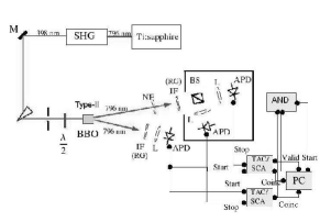
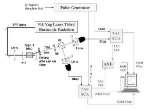
Figure 1: Schematic diagrams of the experimental setups. On the left: setup to reconstruct the joint photon statistics of the bipartite (entangled) states obtained by splitting a PDC-II heralded single-photon state by balanced and unbalanced beam-splitters. On the right: setup to reconstruct the joint photon statistics of a bipartite (classically correlated) state obtained by splitting a multithermal state by a balanced beam splitter.

In order to test our method we have experimentally performed the reconstruction for different bipartite states. The schematic diagrams of the experimental setups are reported in Fig. 1. As a first test, we use our method to reconstruct the bipartite (entangled) states obtained at the output of a beam splitter fed by the heralded single-photon state generated by parametric down conversion (PDC). In our set-up a 0.2 W, 398 nm pulsed (with 200 fs pulses) laser beam, generated by second harmonic of a titanium - sapphire beam at 796 nm, pumps a type II BBO 5x5x1 mm crystal. Upon detecting a photon in a branch of the degenerate PDC emission one triggers the presence of the correlated photon in the other direction. The heralded single-photon is then impinged onto a beam splitter (BS) with unexcited second port, thus generating a bipartite entangled state of the form $|\psi\rangle\rangle=\sqrt{\tau}|01\rangle\rangle\pm\sqrt{1-\tau}|10\rangle\rangle$, $\tau$ being the transmissivity. After the BS both arms are measured by an on/off detectors. All the detectors were APD silicon photodetectors, whose quantum efficiency has been calibrated with the traditional PDC scheme pdccs . The proper set of quantum efficiencies is obtained by inserting before the BS several Schott neutral filters (NF) of different transmittance, evaluated by measuring the ratio between the counting rates with the filter inserted and without it. The data for the reconstruction have been taken using $K=34$ values of $\eta$ from $\eta_{\min}=0.015$ to $\eta_{\max}=0.325$. In correspondence of the detection of a photon in arm 1, a coincidence window has been opened on both detectors on arm 2. This is obtained by sending the output of the first detector as start to two Time to Amplitude Converters (TAC) that receive the detector signal as stop. The 20 ns window is set to not include spurious coincidences with PDC photons of the following pulse (the repetition rate of the laser is 70 MHz). The TAC outputs are then addressed both to counters and to an AND logical gate for measuring coincidences between them. These outputs, together with one TAC Valid Start (giving us the total number of opened coincidence windows), allows to evaluate the frequencies on/off $h_{\mu}$ needed for reconstructing the joint photon statistics of the bipartite state. The background has been evaluated and subtracted by measuring the TAC and AND outputs out of the triggered window.

In order to verify the method in different cases we considered 4 different alternatives given by the combination of a balanced ($\tau=0.5$) or unbalanced ($\tau=0.4$) BS with either large band, red glass filters (RG) with cut-off wave length at 750 nm, or interference filters (IF), with peak wave length at 796 nm and a 10 nm FWHM. The reconstructed statistics for these four situations are shown in Fig. 2. The uncertainties have been evaluated as described in Ref. nos .

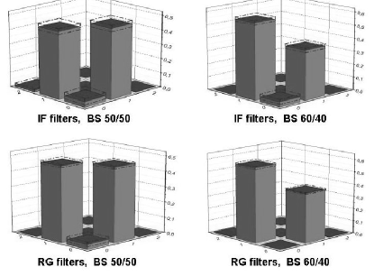
Figure 2: Reconstruction of the joint photon distribution of a bipartite state: PDC heralded photon state split by a beam splitter (balanced and unbalanced). Dashed lines represent one standard deviation.

As it is apparent from Fig. 2 the reconstructed state well corresponds to a single photon in one of the modes. Only the elements $\varrho_{01}$, $\varrho_{10}$ are different (within uncertainties) from zero and their ratio is the value expected by the ratio of the outputs ports of the BS (unity for the balanced one, 2/3 for the unbalanced one). As expected in this regime, no multi-photon component is observed: i.e. $\varrho_{11}$, $\varrho_{20}$, $\varrho_{02}$, and so on are zero within uncertainties. The small uncertainties show that also less unbalanced BS would be distinguishable.

As a second example we consider a single branch of PDC emission without triggering, which corresponds to a multithermal state with number of modes of the order of $\sim 10^{3}$. A bipartite state is generated by impinging this signal onto a beam splitter with the second port unexcited. The output bipartite state is classically correlated (not entangled, but not factorisable), with the two partial traces corresponding to multithermal states. The expected on/off statistics is given by

$$p_{00\eta} =\mu^{\mu}(\mu+\eta N)^{-\mu}$$ (10)

$$p_{01\eta} =\mu^{\mu}\left[(\mu+\eta\tau N)^{-\mu}-(\mu+\eta N)^{-\mu}\right]$$ (11)

$$p_{10\eta} =\mu^{\mu}\left[(\mu+\eta(1-\tau)N)^{-\mu}-(\mu+\eta N)^{-\mu}\right]$$ (12)

respectively, where $N$ is the average number of photons and $\mu$ the number of modes.

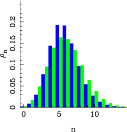
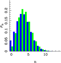
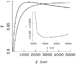
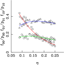
Figure 3: Reconstruction of the joint photon distribution of a bipartite state: attenuated PDC multithermal distribution split by a balanced beam splitter. The two histograms correspond to reconstructed distributions (dark gray) compared to multithermal ones. On the bottom left: fidelity $F$ of the reconstructed marginal distributions to multithermal ones as a function of the number of the iterations of the algorithm. The inset show the total error $\epsilon$. The last box show the measured frequencies $f_{00},f_{01},f_{10}$ as function of the quantum efficiency compared with the expected ones (multithermal, solid lines).

In this case the state has been produced by pumping a 5x5x5 mm type I BBO crystal by a beam of a Q-switched triplicated (to 355 nm) Neodimium-Yag laser with pulses of 5 ns, power up to 200 mJ per pulse and 10 Hz repetition rate. Due to the very high power of the pump beam, a state with a large number of photons is generated. We have therefore attenuated (by 1 nm FWHM IF and neutral filters) the multithermal state before splitting and detection. Measurements at the different quantum efficiencies has been obtained by inserting (before the BS) Schott neutral filters, whose calibration has been obtained by measuring the power of a diode laser (at the same wave length of the used PDC emission) before and after them. The data for the reconstruction has been taken using $K=35$ values of $\eta$ from $\eta_{\min}=0.05$ to $\eta_{\max}=0.25$. The coincidence scheme has been realized by addressing two Q-switch triggered pulses to two TAC modules as starts, and the detectors outputs as stops. Then, having set properly a 20 ns coincidence window, we sent the two TAC outputs to an AND logic port, and the Valid Stops to counting modules (together with one TAC Valid Start and the AND output). The results of this reconstruction are shown in Fig. 3. Also in this case the comparison among theoretical expectations and reconstructed statistics is rather good. The fidelity $F=\sum_{n}\sqrt{\varrho_{n}\varrho_{n}^{mth}}$ of the reconstructed distribution to the expected multithermal $\{\varrho_{n}^{mth}\}$is larger than $99\%$ for both the marginals. Notice that the optimal number of iterations (i.e. leading to maximum average fidelity of the two marginals) corresponds to the minimum of $\epsilon$, thus confirming the good convergence properties of the algorithm.

In conclusion, we demonstrated a method to reconstruct the joint photon statistics of two or more modes using on/off photodetection. Experimental reconstruction have been presented for the bipartite states obtained after a beam-splitter fed by a single photon state or a thermal state. Our results clearly show that the ML reconstruction based on on/off detection can be successfully applied to measure the joint photon statistics for multipartite systems.

This work has been supported by MIUR (FIRB RBAU01L5AZ-002 and RBAU014CLC-002, PRIN 2005023443-002 and 2005024254-002), by Regione Piemonte (E14), and by ”San Paolo foundation”.

References

- (1) See e.g. M. Genovese, Phys. Rep. 413, 319 (2005).
- (2) V. C. Usenko et al., Phys. Lett. A 348, 1723 (2005); A. Porzio et al, Opt. Las. Eng. (2006), in press.
- (3) A. Gatti et al, Phys. Rev. Lett. 93, 093602 (2004).
- (4) B. E. A. Saleh, B. M. Jost, H.-B. Fei, and M. C. Teich, Phys. Rev. Lett 80 3483 (1998).
- (5) G. Zambra et al, Rev. Sci. Instrum. 75, 2762 (2004), J. Kim et al., Appl. Phys. Lett. 74, 902 (1999); A. Peacock et al., Nature 381, 135 (1996); F. Zappa et al., Opt. Eng. 35, 938 (1996); D. Achilles et al., Opt. Lett. 28, 2387 (2003). G. Di Giuseppe et al in Quantum Information and Computation, E. Donkor et al. (Eds.), Proc. SPIE 5105, 39 (2003).
- (6) M. Munroe et al., Phys. Rev. A 52, R924 (1995); Y. Zhang et al., Opt. Lett. 27, 1244 (2002); M. Raymer and M. Beck in Quantum states estimation, M. G .A Paris and J. Řeháček (Eds.), Lect. Not. Phys. 649 (Springer, Berlin-Heidelberg, 2004).
- (7) G. Zambra et al., Phys. Rev. Lett. 95, 063602 (2005); G. Brida et al., Las. Phys. 16, 385 (2006); G. Brida et al., quant-ph/0606046, Op. Syst. Inf. Dyn., in press.
- (8) D. Mogilevtsev, Acta Phys. Slov. 49, 743 (1999); A. R. Rossi et al., Phys. Rev. A 70, 055801 (2004).
- (9) J. ehek et al., Phys. Rev. A 67, 061801(R) (2003).
- (10) K. Banaszek, I. A. Walmsley, Opt. Lett. 28, 52 (2003).
- (11) A.P. Dempster et al., J. R. Statist. Soc. B 39, 1 (1977).
- (12) G. Brida et al, , J. Mod. Opt. 47, 2099 (2000); G. Brida et al, Las. Phys. Lett. 3, 115 (2006).