Effective resonant transitions in quantum optical systems: kinematic and dynamic resonances

Abstract

We show that quantum optical systems preserving the total number of excitations admit a simple classification of possible resonant transitions (including effective), which can be classified by analizying the free Hamiltonian and the corresponding integrals of motion. Quantum systems not preserving the total number of excitations do not admit such a simple classification, so that an explicit form of the effective Hamiltonian is needed to specify the allowed resonances. The structure of the resonant transitions essentially depends on the algebraic propereties of interacting subsystems.

1 Introduction

In a direct analogy with classical mechanics, composed systems in quantum optics (which describe interaction between several subsystems) can be divided into two classes: 1) Systems which possess a necessary number of integrals of motion, so that, the classical counterpart is an integrable system; 2) Systems that do not admit a sufficient number of integrals of motions, so that, the classical counterpart is a non-integrable system [1]. A quantum system can have basically two types of integrals of motion: a) Kinematic integrals, which do not depend on the kind of interaction between subsystems, as for instance, the total number of atoms; b) Dynamic integrals which are related to the particular form of interaction between subsystems, as, for instance, a number of excitations preserved in some transitions between the energy levels of the subsystems.

Typical for quantum optical systems dipole-like interactions between two subsystems ($X$ and $Y$) can be described with a generic multichannel Hamiltonian of the following form:

$$H=\sum\limits_{j}\omega_{j}X_{0}^{j}+\sum\limits_{k}\Omega_{k}Y_{0}^{k}+\sum\limits_{j,k}g_{jk}\left(X_{-}^{j}+X_{+}^{j}\right)\left(Y_{-}^{k}+Y_{+}^{k}\right),$$ (1)

where the two first terms represent the free Hamiltonians of the subsystems, so that the frequencies $\omega_{j},\Omega_{k}\geq 0$, and the last term describes the interaction between them. The operators $X_{0,\pm}^{j}$, $Y_{0,\pm}^{j}$, $[X_{0,\pm}^{j},Y_{0,\pm}^{j}]=0$, are usually elements of some deformed algebra [2], and in particular, satisfy the ladder commutation relations

$$\left[X_{0}^{j},X_{\pm}^{j}\right]=\pm X_{\pm}^{j},\hskip 7.22743pt\left[Y_{0}^{j},Y_{\pm}^{j}\right]=\pm Y_{\pm}^{j}.$$ (2)

In the interaction Hamiltonian there are two kinds of terms: of the form $X_{-}^{j}Y_{+}^{k}$ and $X_{-}^{j}Y_{-}^{k}.$ It is easy to observe that in the rotating frame, that is, applying the following unitary transformation

$$U=\exp\left(it\left[\sum\limits_{j}\omega_{j}X_{0}^{j}+\sum\limits_{k}\Omega_{k}Y_{0}^{k}\right]\right)$$

to the Hamiltonian (1), the counterrotating terms $\sim X_{-}^{j}Y_{-}^{k}$ oscillate in time with a frequency $\omega_{j}+\Omega_{k}$ and the rotating terms $\sim X_{-}^{j}Y_{+}^{k}$ oscillate with a frequency $\omega_{j}-\Omega_{k}$. It is clear that under the condition $\omega_{j}\approx\Omega_{k}$ the rotating term $X_{-}^{j}Y_{+}^{k}$ in (1) is approximately time independent (and thus, can generate transitions with a probability of one between the energy levels of the system), meanwhile the counterrotating term, $X_{-}^{j}Y_{-}^{k}$ always oscillates rapidly in the rotating frame, and its temporal average is zero.

By neglecting the counterrotating terms in the Hamiltonian (1), which is commonly called the Rotating Wave Approximation (RWA), we arrive at the Hamiltonian

$$H=\sum\limits_{j}\omega_{j}X_{0}^{j}+\sum\limits_{k}\Omega_{k}Y_{0}^{k}+\sum\limits_{j,k}g_{jk}\left(X_{-}^{j}Y_{+}^{k}+X_{+}^{j}Y_{-}^{k}\right),$$ (3)

which admits several dynamic integrals of motion $N_{p}$, generally not allowed in (1). This implies that the whole representation space of the system is divided into finite dimensional invariant subspaces, and the mathematical treatment is essentially simplified.

It is worth noting, that the semiclassical models, when some of the subsystems are described by $c$-numbers instead of operators, are treated using essentially the same type of Hamiltonians as (1). The semiclassical transition in (1) can be done by going to the rotating frame of the semiclassical system and then, just substituting the transition operators by some complex numbers. For instance, in the case of single channel interaction, $j=1$, $k=1$, when the system $Y$ acquires classical features, the Hamiltonian (1) in the rotating frame corresponding to the system $Y$ takes the form

$$H=\omega X_{0}+g\left(X_{-}+X_{+}\right)\left(Y_{-}e^{i\Omega t}+Y_{+}e^{-i\Omega t}\right),$$

so that the corresponding semiclassical Hamiltonian is obtained by substituting $Y_{+}\rightarrow g,Y_{-}\rightarrow g^{\ast},$ giving

$$H_{sc}=\omega X_{0}+g\left(X_{-}+X_{+}\right)\left(g^{\ast}e^{i\Omega t}+ge^{-i\Omega t}\right).$$ (4)

Such Hamiltonians usually appear when a quantum oscillator and/or a collection of atoms is pumped by an external force [3], [4], [5].

In the RWA-like systems, described by Hamiltonians of the form (3), the resonance conditions

$$\omega_{j}\approx\Omega_{k},$$ (5)

means that the term $X_{-}^{j}Y_{+}^{k}$, which explicitly appears in the Hamiltonian, does not depend on time in an appropriate rotating frame. Nevertheless, such explicit resonances are not the only kind of resonances, which can be found in the Hamiltonian (3). Usually, the composed systems admit several types of implicit resonances related to effective transitions, which do not appear in the original Hamiltonian, between their energy levels. Such effective interactions play important roles in many physical applications and can be revealed by adiabatic elimination of slow transitions [6]. The implicit (effective) resonances are characterized by their position, $\sum_{j}m_{j}\omega_{j}\approx\sum_{k}n_{k}\Omega_{k}$, and strength, i.e. in what order of perturbation expansion they appear for the first time. Although, a generic system can possess a large number of different types of effective transitions, all the possible resonance conditions can be classified only by analyzing the free Hamiltonian and the integrals of motion. Because all the invariant subspaces are finite-dimensional, there are always a finite number of different resonances. We will refer to these kinds of resonances as kinematic resonances, which include both explicit and implicit resonances. In Sec. II we show with the example of atom-field interactions, that it is possible to classify all the kinematic resonances in a straightforward way.

The situation is quite different in quantum systems with a lack of integrals of motion, corresponding to classically non-integrable dynamic systems. In such systems an infinite number of different resonances arise and a priori it is impossible to determine their position and strength, which essentially depend not only on the type of interaction but also on the algebraic properties of each interacting subsystem [7], [8], [9]. In Sec.III we will discuss such dynamic resonances analyzing different models of interaction of quantum and classical fields with atomic systems.

2 Kinematic resonances

2.1 A simple model

An important example of kinematic resonances is the Dicke Model [10], this model describes the interaction of a collection of $A$ identical two-level atoms with a single mode of a quantized field under the Rotating Wave Approximation. The Hamiltonian that governs this system is given by

$$H=\omega a^{\dagger}a+\omega_{0}S_{z}+g(aS_{+}+a^{\dagger}S_{-}),$$ (6)

where $\omega$ is the field frequency, $\omega_{0}$ is the atomic frequency, and $S_{z}=\sum\limits_{i=1}^{A}s_{zi},S_{\pm}=\sum\limits_{i=1}^{A}s_{\pm i}$ are the collective atomic operators, they represent the atomic inversion, and the transition between the atomic energy levels respectively, their commutation relations are given by the $su(2)$ algebra,

$$\left[S_{z},S_{\pm}\right]=S_{\pm},\quad\left[S_{+},S_{-}\right]=2S_{z},\quad$$ (7)

and $a^{\dagger},a$ are the creation-annihilation field operators, obeying the bosonic commutation relations, $[a,a^{\dagger}]=1$.

The Hamiltonian (6) admits two integrals of motion, a kinematic integral of  motion, given by the total number of atoms (that is constant for a closed system), $A=S^{11}+S^{22}$, where $S^{ii}$ is the atomic population operator for the $i$-th atomic energy level, and the dynamic integral of motion, corresponding to the total number of excitations, has the form

$$N=S_{z}+a^{\dagger}a,\qquad[N,H]=0.$$ (8)

This system is the simplest non trivial example of one-channel quantum transitions: an absorption of one photon is accompanied by an excitation of one atomic transition. Using the integral of motion (8), the Hamiltonian (6) can be rewritten as follows,

$$H=\omega N+H_{int},$$

where the interaction Hamiltonian is

$$H_{int}=\Delta S_{z}+g(aS_{+}+a^{\dagger}S_{-}),\quad$$ (9)

and $\Delta=\omega_{0}-\omega$, is the detuning between the field and the atomic transition frequencies. If the only possible resonant condition, $\omega=\omega_{0},$ is held, the interaction Hamiltonian (9) is reduced to,

$$H_{int}=g(aS_{+}+a^{\dagger}S_{-}),$$ (10)

which implies that the atomic transition probability (as a function of time) oscillates between zero and one.

On  the other hand, in the far-off resonant (dispersive) limit, $|\Delta|\gg g\sqrt{\bar{n}}$, the interaction Hamiltonian (9) is diagonal,

$$H_{int}\simeq\Delta S_{z}+\frac{g^{2}}{\Delta}\left[(2a^{\dagger}a+1)S_{z}-S_{z}^{2}\right],$$ (11)

so that only the phase of the system evolves due to the appearance of the so-called dynamic Stark shift terms [11], [12] in the effective Hamiltonian (11).

2.2 Generic atom-field interactions

Let us consider the interaction of a system of $A$ identical $N$-level atoms of an arbitrary configuration with a single mode of a quantized field of frequency $\omega$. The Hamiltonian describing this system has the form

$$H=H_{d}+H_{int},$$ (12)

where

$$H_{d}=\omega a^{\dagger}a+\sum\limits_{j=1}^{N}E_{j}S^{jj},\hskip 7.22743ptE_{j}<E_{j+1},$$ (13)

is the free Hamiltonian, and $S^{jj}$ are the collective atomic population operators corresponding to the $j$-th atomic level of energy $E_{j}$, and $H_{int}$ is the interaction atom-field Hamiltonian, whose explicit form depends on the atomic configuration, in the dipole approximation, i.e. only one-photon transitions are allowed. In this Section we suppose that the Rotating Wave Approximation is imposed, so that the total number of excitations in the atom-field system is preserved, and thus, the whole representation space of this quantum system is divided into finite-dimensional invariant subspaces.

The Hamiltonian (12) admits two integrals of motion: a kinematic integral, given by the total number of atoms:

$$A=\sum\limits_{i=1}^{N}S^{ii},$$ (14)

and a dynamic integral, corresponding to the total number of excitations in the system:

$$N=a^{\dagger}a+\sum\limits_{i=1}^{N}\mu_{j}S^{ii},$$ (15)

where the parameters $\mu_{j}$ depend on the atomic configuration.

Let us note that a generic interaction term can be written as follows

$$f(S^{ii},a^{\dagger}a)\prod\limits_{j=1}^{N-1}\left(S_{+}^{jN}\right)^{k_{j}}a^{k_{N}},\hskip 7.22743ptk_{j}\in Z\ \forall\ j=1,...,N,$$ (16)

where $S_{\pm}^{ij}$ ($S_{+}^{ij}=S^{ij},$ $S_{-}^{ij}=S^{ji}$, $j>i$) are the atomic transition operators satisfying the $u(N)$ commutation relations, $\left[S^{ij},S^{km}\right]=\delta_{im}S^{kj}-\delta_{kj}S^{im}$, and negative exponents correspond to the Hermitian conjugated operators. The operational coefficients $f(S^{ii},a^{\dagger}a)$ depend on diagonal atomic operators and the photon number operator. In what follows we will omit the coefficient $f(S^{ii},a^{\dagger}a)$, since it leads only to some phase shifts and does not change the distribution of excitations in the system´s energy levels. It is worth noting that (16) is not a unique way to represent a generic interaction term.

Since the Rotating Wave Approximation is imposed, every interaction term should preserve the total number of excitations, so the condition

$$\left[N,\prod\limits_{j=1}^{N-1}\left(S_{+}^{jN}\right)^{k_{j}}a^{k_{N}}\right]=0,$$

is held, and thus, the numbers $k_{j}$ satisfy the following restriction

$$k_{N}=\sum_{j=1}^{N-1}k_{j}\left(\mu_{N}-\mu_{j}\right).$$ (17)

Thus, any admissible interaction can be described as

$$\prod\limits_{j=1}^{N-1}\left(S_{+}^{jN}\right)^{k_{j}}a^{\sum\limits_{j=1}^{N-1}k_{j}\left(\mu_{N}-\mu_{j}\right)}.$$ (18)

The interaction (18) becomes resonant when the atomic transition energies and the field frequency satisfy the following condition

$$\sum\limits_{j=1}^{N-1}k_{j}\left(E_{N}-E_{j}-\omega\left(\mu_{N}-\mu_{j}\right)\right)=0.$$ (19)

The important point here is that interaction terms (18) can be explicitly presented in (12), or can describe effective interactions, and thus should be obtained from the original Hamiltonian by adiabatic elimination of some far-off resonant transitions. So that, the condition (19) describes explicit resonances if the corresponding interaction term is present in the original Hamiltonian or implicit resonances, if such interaction is effective. It is clear that the total number of both explicit and implicit resonances is finite, which is a consequence of the restriction (17) imposed by the Rotating Wave Approximation.

The number of possible resonances depends on the number of atomic levels, $N$, and the total number of atoms, $A$. Note that the resonance condition (19) is associated with a vector $\vec{k}=\left(k_{1},...k_{N-1}\right)$, in order to not repeat the resonances, we consider only vectors $\vec{k}$ with coprime components (that is $k_{1},...k_{N-1}$ do not have a common factor). Then, different vectors $\vec{k}$  satisfying the following condition

$$\max\left\{\left|\sum\limits_{i=1}^{N-1}k_{i}\right|,\left|\sum\limits_{i=1,j\neq i}^{N-1}k_{i}\right|_{j=1,...,N-1},....,\left|k_{i}\right|_{i=1,...,N-1}\right\}\leq A,$$ (20)

define different resonances.

On the other hand, taking into account the dynamic integral of motion (15), one can rewrite the free Hamiltonian (13) as follows,

$$H_{d}=\omega N+\sum\limits_{j=1}^{N}\left(E_{j}-\mu_{j}\omega\right)S^{jj}.$$ (21)

Summing the kinematic integral $-\beta\sum_{i=1}^{N}S^{ii}$ (14) to the above Hamiltonian, where the constants $\beta=\beta(\vec{n}),\vec{n}=(n_{1},..,n_{N})$, are chosen such that,

$$\beta(\vec{n})=\sum\limits_{j=1}^{N}n_{j}\left(E_{j}-\mu_{j}\omega\right),\hskip 7.22743pt\sum\limits_{j=1}^{N}n_{j}=1,\quad n_{j}\in\mathcal{Z},$$

we obtain

$$H_{d}=\omega N+\sum\limits_{j=1}^{N}\left(E_{j}-\mu_{j}\omega-\beta(\vec{n})\right)S^{jj}.$$ (22)

It is easy to see that the condition $E_{j}-\mu_{j}\omega-\beta(\vec{n})=0,$ for any fixed $j$ and some values of $\beta(\vec{n})$, enumerates all the possible resonances (19). Let us take for instance $j=1,$ if $E_{1}-\mu_{1}\omega-\beta(\vec{n})=0,$ then

$$\sum\limits_{j=2}^{N-1}n_{j}\left(E_{N}-E_{j}-\omega\left(\mu_{N}-\mu_{j}\right)\right)+\left(n_{1}-1\right)\left(E_{N}-E_{1}-\omega\left(\mu_{N}-\mu_{1}\right)\right)=0,$$

which coincides with (19), when $k_{j}=n_{j}$ for $j=2,...N-1$ and $k_{1}=\left(n_{1}-1\right)$.

This means that we can always represent the free Hamiltonian in a way that all the possible resonance conditions, corresponding to both explicit and implicit resonances, appear as zeros of coefficients of the atomic population operators $S^{jj}$ in the free Hamiltonian, after taking out the integral of motion (15) corresponding to the total number of excitations.

The above allows us to classify all the possible kinematic resonances:

1. Multiphoton resonances: transitions which involve absorption and emission of photons: a) simple $n$-photon transitions, described by the terms $\sim a^{n}S_{+}^{kj}$, with the resonance condition $E_{j}-E_{k}\approx n\omega$. The terms with $n=1$ can be present in the original Hamiltonian and in such case represent explicit resonances. Multiphoton transitions appear even in a single atom case; b) Collective atomic transitions, described by the terms $\sim a^{n}S_{+}^{kl}S_{-}^{ji},$ (in general a product of several, up to $A$ atomic transition operators can appear), with the corresponding resonance condition $\left(E_{l}-E_{k}\right)-\left(E_{i}-E_{j}\right)\approx n\omega$. It is clear that such resonances can appear only in multi-atom systems. Note, that if $l=i$ (or $k=j$) then we obtain the same resonance condition as in a), describing an effective process of absorption of $n$ photons with atomic transition from $k$-th to $j$-th energy levels. Nevertheless, the corresponding term in the effective Hamiltonian would be multiplied by the atomic population operator $S^{ll}$, which means that more than one atom is need to realize such a process.

2. Virtual photon resonances: atomic transitions between independent channels caused by the quantum field fluctuations, and thus existing even when the field is in the vacuum state. Such resonances appear only when the system has more than one atom and are described by terms in the form of products of atomic transitions operators. For instance, the simplest term of this kind (typically appearing in the first order perturbation expansion) is $S_{+}^{kj}S_{-}^{il}$, $k\neq i$, $j\neq l$, describes atomic transitions $k\rightarrow j$, $l\rightarrow i$, and the corresponding resonance condition is

   $$\left(E_{j}-E_{k}\right)-\left(E_{l}-E_{i}\right)\approx 0.$$ (23)

   Obviously, such transitions can be realized in a system which consists of at least two atoms. Note that the term $\sim S_{+}^{lj}S_{-}^{ik},$ which represents the atomic transition $k\rightarrow i$, $l\rightarrow j$, satisfies the same resonant condition. More involved interactions, like$\sim S_{+}^{ij}S_{-}^{kl}S_{-}^{mn}$, can appear in the highest orders of the perturbation theory. The strength of virtual photon transitions does not depend on the field intensity in the leading order of the perturbation expansion.

3. Photon assisted transitions: atomic transitions when every photon emission is accompanied by a simultaneous photon absorption. These transitions appear only when the atomic configuration contains coherent channels, similar to lambda-like configurations. The strength of such interactions depends on the number of photons in the field and the populations of some atomic energy levels. The simplest terms describing the photon assisted transition (which appear in the lowest order of the perturbation theory) have the form: $f(a^{\dagger}a,S^{jj})S_{+}^{kl}$, corresponding to the resonance condition $E_{l}\approx E_{k}$, where the transition $k\leftrightarrow l$ is not present in the original Hamiltonian and $f(a^{\dagger}a,S^{jj})$ is a linear polynomial of the photon number operator and the atomic population operators.

In the above classification we do not consider interactions corresponding to powers of terms describing some interactions. For instance, the $n$-photon transition corresponding to the term $(aS_{+}^{jk})^{n},$ that describes an absorption of $n$ photons by at least $n$ atoms in the transition $j\rightarrow k$, we include in ”one photon transitions”.

In the case of interaction of an atomic system with classical field the Rotating Wave Approximation implies that the interaction Hamiltonian can always be reduced to a time-independent form. In this case, apart from explicit resonances, several types of implicit (effective) resonant transitions can take place. It is clear that no interactions similar to virtual photon resonances can arise. Nevertheless, transitions similar to multiphoton resonances $\sim S_{+}^{jk},k-j\geq 2$ and photon assisted resonances $\sim S_{+}^{jk}$, where the transition $k\leftrightarrow j$ does not exist in the initial Hamiltonian, actually appear.

2.3 Four level diamond configuration atoms

As an example of the kinematic resonances we will study the interaction of $A$ four level diamond configuration atoms with a single mode of a quantized field under RWA. The Hamiltonian governing the evolution of this system has the form

$$H = \omega a^{\dagger}a+\sum\limits_{j=1}^{4}E_{j}S^{jj}+g_{1}\left(aS_{+}^{12}+a^{\dagger}S_{-}^{12}\right)+g_{2}\left(aS_{+}^{13}+a^{\dagger}S_{-}^{13}\right)$$

$$+g_{3}\left(aS_{+}^{24}+a^{\dagger}S_{-}^{24}\right)+g_{4}\left(aS_{+}^{34}+a^{\dagger}S_{-}^{34}\right).$$

This Hamiltonian describes four one-photon atomic transitions, ($1\leftrightarrow 2$, $1\leftrightarrow 3)$, ($2\leftrightarrow 4$, $3\leftrightarrow 4)$, gathered in two pairs of coherent quantum channels. The corresponding resonance conditions (explicit resonances) are $E_{2}-E_{1}\approx\omega$, $E_{3}-E_{1}\approx\omega$, $E_{4}-E_{2}\approx\omega$, and $E_{4}-E_{3}\approx\omega$. To find all the other (implicit) resonances we will follow the method outlined in previous Subection. The dynamic integral of motion for this system is

$$N=a^{\dagger}a+S^{44}-S^{11},$$

so that the coefficients $\mu_{j}$ in (15), are $\mu_{1}=-1$, $\mu_{2}=\mu_{3}=0$, $\mu_{4}=1$. Substituting these $\mu_{j}$ into (19) we obtain all the possible resonance conditions:

$$k_{1}\left(E_{4}-E_{1}-2\omega\right)+k_{2}\left(E_{4}-E_{2}-\omega\right)+k_{3}\left(E_{4}-E_{3}-\omega\right)\approx 0,$$ (25)

$k_{1},k_{2},k_{3}\in\mathcal{Z},$ and the corresponding (effective) interactions are

$$\left(S_{+}^{14}\right)^{k_{1}}\left(S_{+}^{24}\right)^{k_{2}}\left(S_{+}^{34}\right)^{k_{3}}a^{k_{3}+k_{2}+2k_{1}}.$$

The vector $\vec{k}=\left(k_{1},k_{2},k_{3}\right)$ associated with possible resonances should satisfy the condition (20)

$$\max\left\{\left|\sum\limits_{i=1}^{3}k_{i}\right|,\left|k_{i}+k_{j}\right|_{i\neq j},\left|k_{i}\right|\right\}\leq A,\ \ \ \ i,j=1,2,3.$$

For a single atom we have the vectors $\left(1,0,0\right)$, $\left(0,1,0\right)$, $\left(0,0,1\right)$, $\left(1,-1,0\right)$, $\left(1,0,-1\right)$, $\left(0,1,-1\right)$, which correspond to the following resonance conditions (interactions): $E_{4}-E_{1}\approx 2\omega$ $\left(a^{2}S_{+}^{14}\right)$, $E_{4}-E_{2}\approx\omega$ $\left(aS_{+}^{24}\right)$, $E_{4}-E_{3}\approx\omega$ $\left(aS_{+}^{34}\right)$, $E_{2}-E_{1}\approx\omega$ $\left(aS_{+}^{12}\right)$, $E_{3}-E_{1}\approx\omega$ $\left(aS_{+}^{13}\right)$, $E_{3}\approx E_{2}$ $\left(S_{+}^{23}\right)$, respectively. For two atoms there there are 15 other vector apart from 6 shown above.

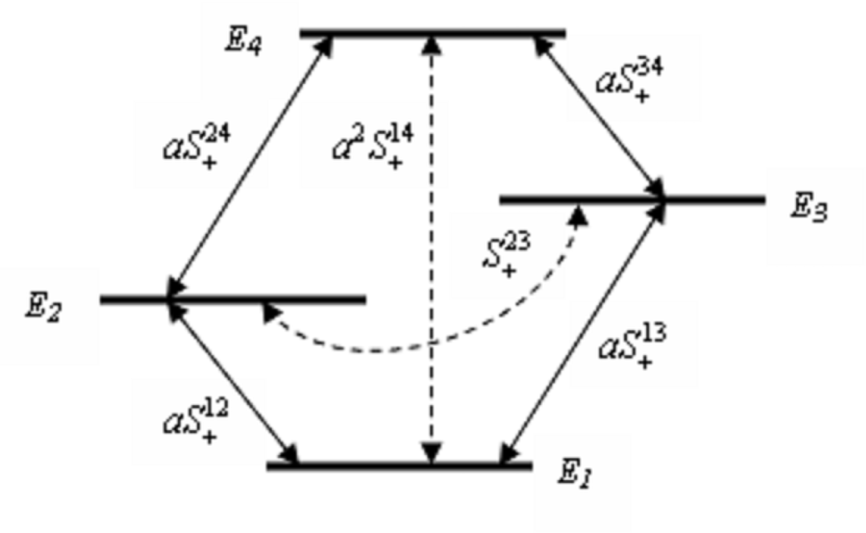
Figure 1: Interactions diagram for a single four level atom of diamond configuration. Solid line: explicit resonances. Dashed line: Implicit resonances: two photon transition, photon assisted transition.

For a better understanding of the nature of the implicit resonances, we find the first order effective Hamiltonian considering that all the interactions appearing in the initial Hamiltonian (2.3) are far from resonance. Following the method outlined in the Appendix, we apply to the Hamiltonian (2.3) the following sequence of unitary transformations

$$H_{eff}=U_{4}U_{3}U_{2}U_{1}HU_{1}^{\dagger}U_{2}^{\dagger}U_{3}^{\dagger}U_{4}^{\dagger},$$

where $U_{i}=\exp\left(\varepsilon_{i}A_{i}\right),$

$$A_{1} = aS_{+}^{12}-a^{\dagger}S_{-}^{12},\ \ \ \ A_{2}=aS_{+}^{13}-a^{\dagger}S_{-}^{13},$$

$$A_{3} = aS_{+}^{24}-a^{\dagger}S_{-}^{24},\ \ \ \ A_{4}=aS_{+}^{34}-a^{\dagger}S_{-}^{34},$$

and the small parameters $\varepsilon_{i}\ll 1$ are given by

$$\varepsilon_{1} = \frac{g_{1}}{E_{2}-E_{1}-\omega},\ \ \ \ \varepsilon_{2}=\frac{g_{2}}{E_{3}-E_{1}-\omega},$$

$$\varepsilon_{3} = \frac{g_{3}}{E_{4}-E_{2}-\omega},\ \ \ \ \varepsilon_{4}=\frac{g_{4}}{E_{4}-E_{3}-\omega},$$

we obtain, in the first order on small parameters, the following effective Hamiltonian

$$H = \omega a^{\dagger}a+\sum\limits_{j=1}^{4}E_{j}S^{jj}+\Phi(a^{\dagger}a,S^{jj})+g_{2}\varepsilon_{1}\left[S_{+}^{23}\left(S^{11}+a^{\dagger}a+1\right)+h.c.\right]$$ (26)

$$+g_{4}\varepsilon_{3}\left[S_{+}^{23}\left(S^{44}-a^{\dagger}a\right)+h.c.\right]-\left(g_{3}\varepsilon_{1}+g_{4}\varepsilon_{2}\right)\left(a^{2}S_{+}^{14}+h.c.\right)$$

$$+g_{3}\varepsilon_{1}\left(S_{+}^{24}S_{-}^{12}+h.c.\right)+g_{3}\varepsilon_{2}\left(S_{+}^{24}S_{-}^{13}+h.c.\right)$$

$$+g_{4}\varepsilon_{1}\left(S_{+}^{12}S_{-}^{34}+h.c.\right)+g_{4}\varepsilon_{2}\left(S_{+}^{13}S_{-}^{34}+h.c.\right).$$

where

$$\Phi(a^{\dagger}a,S^{jj}) = g_{1}\varepsilon_{1}\left(S^{22}\left(S^{11}+1\right)+a^{\dagger}a\left(S^{22}-S^{11}\right)\right)$$

$$+g_{2}\varepsilon_{2}\left(S^{33}\left(S^{11}+1\right)+a^{\dagger}a\left(S^{33}-S^{11}\right)\right)$$

$$+g_{3}\varepsilon_{3}\left(S^{44}\left(S^{22}+1\right)+a^{\dagger}a\left(S^{44}-S^{22}\right)\right)$$

$$+g_{4}\varepsilon_{4}\left(S^{44}\left(S^{33}+1\right)+a^{\dagger}a\left(S^{44}-S^{33}\right)\right)$$

is the dynamic Stark shift [11].

Let us classify the effective resonances present in the above (first order)Hamiltonian:

1. Multiphoton resonances: The only two resonances of this type are one-photon and two-photon resonances. There are four one-photon transitions corresponding to explicit resonances, which do not appear in the effective Hamiltonian (26). The term $\sim a^{2}S_{+}^{14}$ describes two-photon transitions, with corresponding resonance condition $E_{4}-E_{1}\approx 2\omega$.

2. Virtual photon resonances: the last four terms in (26), $\sim S_{+}^{24}S_{-}^{12}$, $S_{+}^{24}S_{-}^{13}$, $S_{+}^{12}S_{-}^{34}$, $S_{+}^{13}S_{-}^{34}$, with the resonance conditions $E_{4}-E_{2}\approx E_{2}-E_{1}$, $E_{4}-E_{2}\approx E_{3}-E_{1}$, $E_{2}-E_{1}\approx E_{4}-E_{3},$ and $E_{3}-E_{1}\approx E_{4}-E_{3}$ respectively.

3. Photon assisted resonances: The only resonance of this type is of the form $\sim f\left(S^{44},S^{11},a^{\dagger}a\right)S_{+}^{23},$ is produced in the first order of the perturbation theory generating transitions between the middle atomic levels, and the corresponding resonance condition is $E_{3}\approx E_{2}.$

3 Dynamic Resonances

In this Section we study quantum systems corresponding to classically non-integrable systems, mainly focusing on the models describing interaction of atoms with quantized and classical fields without applying the Rotation Wave Approximation [7], [9] (some different systems not preserving the number of excitations are discussed in [8]).

It is convenient to start with a general analysis of such systems. The main idea consists in removing the counter-rotating terms from the multi-channel Hamiltonian (1) using a method of adiabatic elimination. In the limit of weak interaction, $g_{jk}\ll\omega_{n},\Omega_{m}$ one can apply, for instance, the Lie-transformation method outlined in the Appendix. Although, such analysis can be performed for a general system, we will focus on the simplest case of a one channel Hamiltonian and show, that even in this case the absence of the integral of motion corresponding to the total number of excitations leads to the appearance of a series of (dynamic) resonances, which can be classified according the interaction type.

Consider a single-channel Hamiltonian (1)

$$H=\omega X_{0}+\Omega Y_{0}+g(X_{+}Y_{-}+X_{-}Y_{+})+g\left(X_{+}Y_{+}+X_{-}Y_{-}\right),$$ (27)

where $X_{0}$ ($Y_{0}$) is the free Hamiltonian of the subsystem $X$ ($Y$) and $X_{+}$ ($Y_{+}$), $X_{-}$ ($Y_{-}$) are the up and down operators (see Appendix), respectively, which describe transitions between the energy levels in the subsystem $X$ ($Y$), they hold the $su_{d}(2)$ [2] commutation relations (2). From now on, we do not impose any commutation relation between the transition operators, which are generally some functions of the diagonal operators and integrals of motion $\left[N_{1},X_{0,\pm}\right]=\left[N_{2},Y_{0,\pm}\right]=0$,

$$\left[X_{+},X_{-}\right] = P_{1}\left(X_{0}\right)=\nabla_{X_{0}}\phi_{1}\left(X_{0},N_{1}\right),$$

$$\left[Y_{+},Y_{-}\right] = P_{2}\left(Y_{0}\right)=\nabla_{Y_{0}}\phi_{2}\left(Y_{0},N_{2}\right).$$

where $\nabla_{X_{0}}\phi_{1}\left(X_{0},N_{1}\right)$, $\nabla_{Y_{0}}\phi_{2}\left(Y_{0},N_{2}\right)$ are given by the structural functions (appendix (48)), and, in general, (we are going to omit the dependence of the integral of motion)

$$\nabla_{z}\phi\left(z\right)=\phi\left(z\right)-\phi\left(z+1\right).$$

The consequences of the existence of the counterrotating term $\sim XY$ in the Hamiltonian (27) are:  a) the dimension of the whole representation space is the product of the corresponding dimensions of the subsystems: $\dim(X\otimes Y)=\dim X\cdot\dim Y$, b) there are some additional resonances apart from $\omega=\Omega$, that in the case of a single-channel Hamiltonian (3) do not exist, c) The type of resonances depends on the structure of algebras describing the $X$ and $Y$  systems.

The counterrotating term rapidly oscillates (with frequency $\omega+\Omega$), and thus, can be eliminated by applying the Lie-type transformation

$$U=\exp\left[\varepsilon\left(X_{+}Y_{+}-X_{-}Y_{-}\right)\right],\quad\varepsilon=g/\left(\omega+\Omega\right)\ll 1,$$ (28)

to the Hamiltonian (27) and using the standard perturbative expansion, see Appendix . From now on we suppose that $\omega\geq\Omega.$

The elimination of the above term leads to the appearance of new elements in the transformed Hamiltonian. All these new terms can be divided into three groups: the first group contains the non-resonant terms, of the form $X_{+}^{n}Y_{+}^{m}+h.c.$, that can always be eliminated under the condition $\omega,\Omega\gg g$ by applying some suitable transformations; the second group consists of resonant terms, that cannot be removed if certain relations between $\omega$ and $\Omega$ hold, since the interaction becomes resonant ( the transformation which eliminates a given term from the Hamiltonian becomes singular). This group contains terms of the form $X_{+}^{n}Y_{-}^{m}+h.c.$, which describe transitions between energy levels of the whole system. The third group includes the diagonal terms (functions only of $X_{0},Y_{0}$), that can never be removed. Our strategy consists of keeping in the Hamiltonian only diagonal terms and resonant terms, and, we conserve only the leading order coefficients in these terms.

All the counterrotating terms, like $\sim$ $X_{+}^{n}Y_{+}^{m},$ can be eliminated by applying the Lie-type transformation

$$U=\exp\left[\pi(\varepsilon_{1}..\varepsilon_{k})\eta\left(X_{+}^{n}Y_{+}^{m}-X_{-}^{n}Y_{-}^{m}\right)\right],$$ (29)

where $\eta\approx g/\left(n\omega+m\Omega\right)\ll 1$, and $\pi(\varepsilon_{1}..\varepsilon_{k})$ is the product of powers of some small parameters $\varepsilon_{j}\ll 1$, $j=1,....,k$. In fact $\pi(\varepsilon_{1}..\varepsilon_{k})$ is proportional to the coefficient of the term $\sim X_{+}^{n}Y_{+}^{m}+X_{-}^{n}Y_{-}^{m}$. Applying a sequence of appropriate transformations (29) we obtain the effective Hamiltonian [7]

$$H_{eff}\approx\omega X_{0}+\Omega Y_{0}+g\varepsilon\Phi\left(X_{0},Y_{0},\varepsilon\right)+$$

$$+g\sum_{k=1}^{\infty}\sum_{l=0}^{\infty}\frac{(-\delta)^{l+k-1}\varepsilon^{l+2(k-1)}}{(k-1)!\left(l+k-1\right)!}\left[X_{+}^{k}Y_{-}^{2l+k}\theta_{kl}(X_{0},Y_{0},\varepsilon)+h.c.\right],$$ (30)

where $\delta=g/2\Omega\ll 1.$

The term $\Phi\left(X_{0},Y_{0},\varepsilon\right)$ represents the dynamic Stark shift (or Bloch-Siegert shift) [13] and can be expanded on powers of the small parameter $\varepsilon$ as follows

$$\Phi\left(X_{0},Y_{0},\varepsilon\right)=\phi_{1}\left(X_{0}\right)\phi_{2}(Y_{0})-\phi_{1}\left(X_{0}+1\right)\phi_{2}(Y_{0}+1)+O(\varepsilon^{2}).$$ (31)

The terms of the form$\ X_{+}^{k}Y_{-}^{2l+k}+h.c.$ describe all the admissible resonant interactions. In particular the term with $k=1$, $l=0$ represents the principal resonance. The coupling constants $\theta_{kl}(X_{0},Y_{0},\varepsilon)$ depend on the algebraic structure (48) of the operators describing both subsystems (more precisely, on the degree of the structural polynomials $\phi_{1}\left(X_{0},N_{1}\right)$ and $\phi_{2}\left(Y_{0},N_{2}\right)$), and in particular, they can become zero for some $k$, $l$ [7]. The coefficient in the principal term has the form

$$\theta_{10}(X_{0},Y_{0})=1,$$

and

$$\theta_{kl}(X_{0},Y_{0})=\sum_{j=0}^{l+[k/2]}C_{l+[k/2]}^{j}\left(P_{1}\left(X_{0}+k\right)\right)^{l+[k/2]-j}\left(-P_{1}\left(X_{0}\right)\right)^{j}R_{k}(X_{0},Y_{0}-2j),$$ (32)

$$R_{k}(X_{0},Y_{0}) = \sum_{j=0}^{[\frac{k-1}{2}]}C_{[\frac{k-1}{2}]}^{j}\left(P_{1}\left(X_{0}+k\right)\right)^{[\frac{k-1}{2}]-j}\left(-P_{1}\left(X_{0}\right)\right)^{j}\nabla_{Y_{0}}^{k-1}\phi_{2}\left(Y_{0}-2j\right)$$

$$\times\prod\limits_{i=1-2j}^{k-2(j+1)}\phi_{2}\left(Y_{0}+i\right),$$

for $l\geq 1$, where $C_{k}^{j}$ are the binomial coefficients and $\nabla_{z}^{0}f(z)=1$. Note that the product in the last equation is equal to unity if the upper limit is less than the lower one.

In contrast to the case of kinematic resonances discussed in the previous Section, the number of possible resonant interactions appearing in the Hamiltonian (30) is infinite. These interactions (dynamic resonances) can be classified as follows: a) Principal (explicit) resonance, $\omega=\Omega,$ corresponding to the interaction term that is explicitly present in the original Hamiltonian $\sim X_{+}Y_{-}$; b) Higher-order resonances: $\left(2l+k\right)\Omega=k\omega$ where $l,k$ $\in N\quad$($l\geq 1,k\geq 1$), corresponding to the effective interactions $\sim X_{+}^{k}Y_{-}^{2l+k}$, which can be divided into: b.1) odd resonances: when $k=1,l=1,2,3,...$, that is $\omega=\left(2l+1\right)\Omega$, b.2) even resonances: $k=2,l=1,3,5...$, with the resonance condition $\omega=2m\Omega,\quad m=1,2,...$, b.3) fractional resonances: $\omega=\left(2l/k+1\right)\Omega,$ where $k$ and $l$ are coprime numbers.

It is worth noting that in the vicinity of each resonance $\left(2l+k\right)\Omega=k\omega$, only the interaction term $\sim X_{+}^{k}Y_{-}^{2l+k}$ survives. This means that if some resonance condition is held, the system is in an approximate invariant subspace and there exists an approximate integral of motion $N=\left(2l+k\right)X_{0}+kY_{0}$.

This simple example shows that even in one-channel systems an infinite number of resonant interactions may arise, if the total number of excitations is not preserved. The appearance of such dynamic resonances in chaotic-like systems is expected from the point of view of classical dynamic systems [1]. Nevertheless, the quantum nature of interacting subsystems imposes certain restrictions on the possibility of surviving of the dynamic resonances. We will discuss such restrictions for two examples of the interaction of an atomic system with quantum and classical fields.

3.1 Atom-quantized field interaction

Let us consider a collection of $A$ identical two-level atoms interacting with a single mode of a quantized field (the Dicke model) without RWA. The Hamiltonian that describes this system is

$$H=\Omega a^{\dagger}a+\omega S_{z}+g(aS_{+}+a^{\dagger}S_{-})+g(a^{\dagger}S_{+}+aS_{-}),$$ (33)

and the condition $\omega,\Omega\gg g$ is held.

The following identifications

$$X_{0}=S_{z},X_{\pm}=S_{\pm},\;Y_{0}=n,Y_{+}=a^{\dagger},Y_{-}=a,$$

so that $\phi_{1}(X_{0})=(1+A/2)A/2-X_{0}^{2}+X_{0},\phi_{2}(Y_{0})=Y_{0},$ lead to $\theta_{kl}\left(S_{z},n\right)=0,\,k\geq 3$ and the effective Hamiltonian (30) takes the form

$$H_{eff} \approx \omega S_{z}+\Omega a^{\dagger}a+g\varepsilon\left(S_{z}^{2}+\left(2a^{\dagger}a+1\right)S_{z}-(1+A/2)A/2\right)$$

$$+g\sum_{l=0}^{\infty}\frac{\left(-2\delta\varepsilon\right)^{l}}{l!}\left[a^{2l+1}S_{+}+h.c.\right]-g\varepsilon\sum_{m=1}^{\infty}\frac{\left(4\delta\varepsilon\right)^{2m}}{(2m)!}\left[a^{4m}S_{+}^{2}+h.c.\right],$$

where $\varepsilon=g/\left(\Omega+\omega\right),\delta=g/2\Omega\ll 1.$

Note that the Hamiltonian (3.1) contains only the principal (explicit) resonance ($l=0$), the even and the odd order interactions, but no fractional resonances. This happens because the structural functions for our subsystems are of a first degree polynomial of the photon number operators $a^{\dagger}a$ and a second degree polynomial of the atomic population operator $S_{z}$.

The integrals of motion for the series of odd and even (exact) resonances are

$$N^{(kl)} = (2l+k)S_{z}+ka^{\dagger}a+2k\delta\left(S_{+}+S_{-}\right)\left(a^{\dagger}+a\right)-$$

$$-\frac{2k^{2}\delta^{2}}{l\left(l+k\right)}\left[\left(2l+k\right)S_{z}\left(2a^{\dagger}a+1\right)-kS_{z}^{2}\right]+O\left(\delta{}^{3}\right),$$

where $l=2m+1$ in $N^{(2l)}$, $m=0,1,2,3,..$ and $k=1,2$ for even and odd resonances correspondingly.

Let us recall that the higher resonances appear in the effective Hamiltonian (3.1) only under the condition $\omega\geq\Omega$. In the opposite case, $\omega\leq\Omega$, only the principal resonance survives and in the approximation (30) the whole effect of the counter-rotating terms reduces to the dynamic Stark shift, which has the same form as in the above case. This does not imply that there are no higher resonances at all, but rather that they are essentially suppressed.

3.2 Atom-classical field interaction

We will proceed with the analysis of the interaction of atomic systems with classical fields without RWA. A generic interaction Hamiltonian has the form

$$H=\sum\limits_{jj}\omega_{j}X_{0}^{j}+\sum_{j}g_{j}\left(X_{j}+X_{j}^{\dagger}\right)\cos(\Omega_{j}t+\vartheta_{j}),$$ (35)

and admits some explicit resonances, $\omega_{j}=\Omega_{j}$. The whole set of effective (implicit) interactions can be easily obtained in the same way as it was outlined in 3.1. To be able to use the effective Hamiltonian in the form (30) we first rewrite the Hamiltonian (LABEL:Hc) in the Floquet form by making use of the phase operators $\{E_{0j},E_{j}\}$, which are generators of the Euclidean algebra:

$$\left[E_{0j},E_{k}\right]=-\delta_{jk}E_{j},\quad\left[E_{0j},E_{j}^{\dagger}\right]=\delta_{jk}E_{j}^{\dagger},\quad\left[E_{j},E_{k}^{\dagger}\right]=0.$$ (36)

Each group of operators (labeled with the same index $j$) acts in a Hilbert space spanned on the eigenstates of the (Hermitian) operator $E_{0j}:$

$$E_{0j}|n\rangle_{j}=n|n\rangle_{j},\quad n=...-1,0,1,...,$$ (37)

so that in the basis (37) the operators $E_{j},E_{j}^{\dagger}$ act as rising-lowering operators:

$$E_{j}|n\rangle_{j}=|n-1\rangle_{j},\quad E_{j}^{\dagger}|n\rangle_{j}=|n+1\rangle_{j}.$$

The phase states $|\vartheta\rangle_{j}$, the eigenstates of $E_{j},$ $E_{j}|\theta\rangle_{j}=e^{-i\vartheta_{j}}|\vartheta\rangle_{j}$, are not normalized.

Now, let us consider the following time independent Hamiltonian

$$H^{op}=\sum_{j}\omega_{j}h_{j}+\sum_{jj}\Omega_{j}E_{0j}+\sum_{j}g_{j}\left(X_{j}+X_{j}^{\dagger}\right)(E_{j}+E_{j}^{\dagger}).$$ (38)

It is easy to observe that the average value of the above Hamiltonian over the phase states in the rotating frame,

$$|\vartheta(t)\rangle = \Pi_{j}e^{-i\Omega_{j}tE_{0j}}|\vartheta\rangle_{j},$$ (39)

$$|\vartheta\rangle_{j} = \lim_{N\rightarrow\infty}\frac{1}{\sqrt{2N+1}}\sum_{n=-\infty}^{\infty}e^{-i\vartheta_{j}n}|n\rangle_{j},$$

where $|n\rangle_{j}$ are the basis states (37), coincides with the Hamiltonian (35) due to

$$\langle\vartheta(t)|E_{0j}|\vartheta(t)\rangle=0,\quad\langle\vartheta(t)|E_{j}|\vartheta(t)\rangle=e^{-i(\Omega_{j}t+\vartheta_{j})}.$$

The Hamiltonian (38) is a Floquet form of the initial time dependent Hamiltonian (35) (from now on we put all the phases $\vartheta_{j}$ equal to zero). In the case of weak driven fields, $g\ll\omega,\Omega$, the Hamiltonian (38) can be represented in a form of expansion over the principal resonances which can be observed in this system according to (30).

In the single channel case, the Dicke model in the classical field, we have the classical problem, first solved by Shirley [3] (for a single two level atom). Let us consider a collection of $A$ two level atoms in a linearly polarized EM field. The corresponding Hamiltonian has the form

$$H=\omega S_{z}+g\left(S_{-}+S_{+}\right)\cos\Omega t,$$ (40)

where $\Omega$ is the classical field frequency.

The Floquet form of (40) is

$$H^{op}=\omega S_{z}+\Omega E_{0}+g\left(S_{-}+S_{+}\right)(E+E^{\dagger}),$$ (41)

The following identifications

$$X_{0}=S_{z},X_{\pm}=S_{\pm},\;Y_{0}=E_{0},Y_{+}=E^{\dagger},Y_{-}=E,$$

so that $\phi_{1}(X_{0})=(1+A/2)A/2-X_{0}^{2}+X_{0},\phi_{2}(Y_{0})=E^{\dagger}E=EE^{\dagger}=I,$ lead to $\theta_{kl}\left(S_{z},n\right)=0,\,k\geq 2$ which immediately leads to the effective Hamiltonian (30)

$$H_{eff}^{op}=\omega S_{z}+\Omega E_{0}+2g\varepsilon E^{\dagger}ES_{z}+g\sum\limits_{l=0}^{\infty}\frac{\left(-2\delta\varepsilon\right)^{l}}{l!}\left(E^{2l+1}S_{+}+h.c.\right).$$ (42)

Averaging the above Hamiltonian over the phase states we obtain an effective time-dependent Hamiltonian

$$H_{eff}=\omega S_{z}+2g\varepsilon S_{z}+g\sum\limits_{l=0}^{\infty}\frac{\left(-2\delta\varepsilon\right)^{l}}{l!}\left(e^{-i(2l+1)\Omega t}S_{+}+h.c.\right),$$

which means that only odd resonances, $\Omega\approx\left(2l+1\right)\omega$, appear in this system. This result is different from the atom-quantum field interaction (and surprisingly can not be obtained from the corresponding quantum Hamiltonian (3.1) by substituting the field operators by $c-$numbers), because in this case the structural function (48) for the Euclidean algebra (36) is a constant, that is, a zero-th degree polynomial function.

4 Conclusions

Quantum systems possessing as the integral of motion the operator corresponding to the total number of excitations (classically integrable systems) admit a simple classification of possible resonant transitions, which are separated into explicit (which appear in the original Hamiltonians) and implicit (effective) resonances. The total number of such resonances is always finite and depends on the number of atoms and of atomic levels. By a simple algebraic manipulation of the free Hamiltonian and the integrals of motion, one can obtain some specific conditions for the frequencies of interacting subsystems, which define the implicit resonances. Nevertheless, the form of the interaction terms associated with each implicit resonance condition can be found only after obtaining the effective Hamiltonian (in a perturbative way).

Quantum systems not preserving the total number of excitations (classically non-integrable systems) do not admit a simple classification of admissible resonant transitions. The explicit form of the effective Hamiltonian is needed to specify the allowed resonances, and their number is always infinite. Such non-linear (on the generators of some Lie algebra) Hamiltonians can be represented as a series of operators describing all the possible transitions, which might become resonant under specific relations between frequencies of interacting subsystems. The structure of the effective Hamiltonian essentially depends on the algebraic structure of interacting subsystems (polynomials $P_{X}\left(X_{0}\right),P_{Y}\left(Y_{0}\right)$). In particular, it is reflected in the types of resonances which are allowed for a given system.

In the vicinity of each resonant transition all of the other transitions can be considered as a perturbation. Thus, in the course of evolution some specific finite-dimensional subspaces in the Hilbert space of the whole system are approximately preserved, and for each of these invariant subspaces there is a corresponding integral of motion.

Acknowledgement 1

This work is partially supported by the Grant 45704 of ConsejoNacional de Ciencia y Tecnologia (CONACyT).

5 Appendix

The method of Lie-type transformation (small rotations) [14], [15] provides a regular procedure for obtaining approximate Hamiltonians describing the effective dynamics of nonlinear quantum systems. The idea of this method is based on the observation that several quantum optical Hamiltonians can be written in terms of polynomially deformed algebras $sl_{pd}(2,R)$ [2], [16], [17], [18], [19], [20],

$$H_{\mathrm{int}}=\Delta\ X_{0}+g\left(X_{+}+X_{-}\right),$$ (43)

where the operators $X_{\pm}$ and $X_{0}$ are generators of the deformed algebra and satisfy the following commutation relations (2), and

$$[X_{+},X_{-}]=P(X_{0}),$$ (44)

where $P(X_{0})$ is a polynomial function of the diagonal operator $X_{0}$ with coefficients that may depend on some integrals of motion $N_{j}.$ If $P(X_{0})$ is a linear function of $X_{0}$, the usual $sl(2,R)$ or $su(2)$ algebras are restored. If for some physical reason (depending on the particular model under consideration) $\eta=g/\Delta\ll 1$ is a small parameter, the Hamiltonian (43) is almost diagonal in the basis of the eigenstates of $X_{0}$ and can be approximately diagonalized by applying in a perturbative manner the following unitary transformation (a small nonlinear rotation)

$$U=\exp\left[\eta\left(X_{+}-X_{-}\right)\right].$$ (45)

Applying the transformation (45) to the Hamiltonian (43) according to the standard expansion

$$e^{A}Be^{-A}=\sum_{k=1}^{\infty}\frac{\eta^{k}}{k!}\mathrm{ad}_{A}^{k}(B),$$ (46)

where $\mathrm{ad}_{A}$ is the adjoint operator defined as $\mathrm{ad}_{A}(B)=[A,B]$, we obtain

$$H_{\mathrm{eff}} = UH_{\mathrm{int}}U^{\dagger}=\Delta\ X_{0}+g\sum_{k=1}^{\infty}\eta^{k}\frac{k}{(k+1)!}\mathrm{ad}_{T}^{k}(X_{+}+X_{-}),$$ (47)

where $T=X_{+}-X_{-}$ and we have taken into account that, due to (44),

$$\mathrm{ad}_{T}(X_{0})=[T,X_{0}]=-\left(X_{+}+X_{-}\right).$$

The effective Hamiltonian acquires the following form

$$H_{\mathrm{eff}}=\Delta\ X_{0}+g\eta\sum_{k=0}^{\infty}{}^{\prime}\eta^{k}\left[X_{+}^{k}f_{k}(X_{0},\eta)+h.c.\right],$$

where $f_{k}(X_{0},\eta)$ is a function of the diagonal operator $X_{0}$ and can be represented as a series on $\eta$:

$$f_{k}(X_{0},\eta)=\frac{2\left(k+1\right)}{\left(k+2\right)!}\nabla^{k+1}\phi(X_{0})+\mathcal{O}(\eta),$$

and

$$\phi(X_{0})=X_{+}X_{-}$$ (48)

is a structural function, $\nabla\phi(X_{0})=\phi(X_{0})-\phi(X_{0}+1)=P(X_{0})$; the prime ( ^′) in the above sum means that the term with $k=0$ is taken with the coefficient $1/2$.

By keeping terms up to order $\eta$ we get

$$H_{\mathrm{eff}}=\Delta\ X_{0}+\eta g\nabla\phi(X_{0}),$$ (49)

and in the first approximation the resulting effective Hamiltonian is diagonal on the basis of eigenstates of $X_{0}$.

The higher-order contributions always have the form $X_{+}^{k}f_{k}(X_{0})+\mathrm{h.c.}+g(X_{0})$. This makes the procedure of removing the off-diagonal terms somehow trivial at each step, in the sense that it is always obvious which transformation should be applied. For example, to eliminate the terms of the form

$$\eta^{l}[X_{+}^{k}f_{k}(X_{0})+f_{k}(X_{0})X_{-}^{k}],$$

it suffices to apply the transformation

$$\exp(\frac{\eta^{l+1}}{k}T_{k}),$$ (50)

with $T_{k}=X_{+}^{k}f_{k}(X_{0})-f_{k}(X_{0})X_{-}^{k}$, since the first commutator of $\Delta\ X_{0}$ with $T_{k}$ cancels the corresponding term in the Hamiltonian.

References

- [1] M.C. Gutzwiller, Chaos in Classical and Quantum Mechanics, Springer (1990).
- [2] V.P. Karassiov, J. Sov. Laser Research 13, 188 (1992); J. Phys. A 27, 153 (1994); B. Abdesselam, J. Beckers, A. Chakrabart, N. Debergh, J. Phys. A 29, 3075 (1996).
- [3] J. H. Shirley, Phys. Rev. 138, B797 (1965).
- [4] C. Cohen-Tannoudji, J. Dupont-Roc and C. Fabre, J.Phys. B 6 (1973) L214.
- [5] T. Yabuzaki, S. Nakayama, Y. Murakami, and T. Ogawa, Phys. Rev. A 10 (1974) 1955 .
- [6] A. Schenzle, A., Nonlinear Optical Phenomena and Fuctuations, Lecture Notes in Physics 155 (Berlin: Springer) (1981) p. 103. Y.R. Shen, The Principles of Nonlinear Optics (New York: John Wiley) (1985). L.A. Lugiato, P. Galatola, and L.M. Narducci 1990, Opt. Commun., 76, 276 (1990). L. Sczaniecki, Phys. Rev. A 28, 3493 (1983). M. Hillery, and L.D. Mlodinow, 1985, Phys. Rev. A, 31, 797 (1985). D.J. Klein, D. , J. Chem. Phys., 61, 786 (1974).
- [7] A.B. Klimov, I. Sainz, S.M. Chumakov, Phys. Rev. A 68, 063811 (2003).
- [8] A.B. Klimov, I. Sainz, C. Saavedra, J. Opt. B: Quant-sem. Opt. 6, 448-453 (2004).
- [9] I. Sainz, A.B. Klimov, C. Saavedra, Phys. Lett. A 351, 26-30 (2006).
- [10] R. Dicke, Phys. Rev. 93, 99 (1954); E.T. Jaynes and F.W. Cummings, Proc. IEEE 5, 89 (1963); B.W. Shore and P.L. Knigth, J. Mod. Opt. 40, 1195 (1993).
- [11] R.R. Puri, R.K. Boullough, J. Opt. Soc. Am. B 5, 2021 (1988).
- [12] A.B. Klimov and C. Saavedra, Phys. Lett. A, 247, 14 (1998).
- [13] F. Bloch and A. Siegert, Phys.Rev. 57, 552 (1940).
- [14] A. B. Klimov and L. L. Sánchez-Soto, Phys. Rev. A 61, 063802 (2000).
- [15] A. B. Klimov, L. L. Sánchez-Soto, A. Navarro, and E. C. Yustas, J. Mod. Opt. 49 (2002).
- [16] P. W. Higgs, J. Phys. A 12, 309 (1979).
- [17] M. Roĉek, Phys. Lett. B 255, 554 (1991).
- [18] D. Bonatsos, C. Daskaloyannis, and G. A. Lalazissis, Phys. Rev. A 47, 3448 (1993).
- [19] E. K. Sklyanin, Funct. Anal. Appl. 16, 263 (1982).
- [20] V. P. Karassiov and A. B. Klimov, Phys. Lett. A 189, 43 (1994).