Conclusive quantum-state transfer with a single randomly coupled spin chain

Abstract

We studied the quantum state transfer in randomly coupled spin chains. By using local memories storing the information and dividing the task into transfer portion and decoding portion, conclusive transfer was ingeniously achieved with just one single spin chain. In our scheme, the probability of successful transfer can be made arbitrary close to unity. Especially, our scheme is a good protocol to decode information from memories without adding another spin chain. Compared with Time-reversed protocol, the average decoding time is much less in our scheme.

PACS: 03.67.Hk, 05.60.Gg, 75,10.Pq

1 Introduction

The task of Quantum state transfer(QST) is to transfer a quantum state from the sender(Alice) to the receiver(Bob). In 2003, Bose [2] presented a scheme to transfer states using unmodulated spin chains. After that, much effort has been devoted to developing this scheme [2-19]. In this scheme, we encode the state at one end of the spin chain and wait for a specific amount of time, then we get the state at another end of the chain. All the operations and measurements are performed at the sending and receiving qubits, but the spin chain connecting them is under no operation.

A simple example of this scheme is a one-dimension spin chain of XY model interaction with equal nearest-neighbor coupling. However, perfect QST can be achieved only when the number of spins is less than four [2, 4]. Based on the Cartesian Product method of the graph theory, Christandl et al [4] extended the case of two or three spins to spin networks which can also get perfect QST. Considering the symmetry of the Hamiltonian(i.e., mirror symmetry, translational symmetry), another approach is to use the Hamiltonians with engineered couplings. Recently, more attention was payed to get perfect QST with randomly coupled quantum spin chains. A “dual-rail” encoding using two parallel quantum channels [11, 12] is suggested to get conclusive and arbitrary perfect QST. Here, the word “conclusive” means whether the state is transferred successfully can be determined by measuring one qubit of Bob’s without destroying the information. Another method is to use local memories [10], by swapping the qubit of Bob to the memory at equal time intervals, the whole information will be stored in the memories and can be decoded by Time-reversed protocol.

The aim of this paper is to replace the “dual-rail” scheme [11] with a single spin chain and reach perfect and arbitrary quantum state transfer. Our scheme also provides a convenient and rapid decoding protocol for ref.[10]. The first step of our scheme is to transfer the information to a collection of memories by continually swapping between Bob and the memories, and the second step is decoding the information from the memories.

2 Our scheme for perfect QST

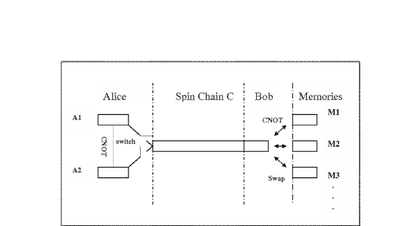
Figure 1: Perfect quantum state transfer in one spin chain using local memories

Our scheme is divided into four parts: A(Alice), B(Bob), C(other parts in the spin chain), M(memories). See Fig.1. A contains two identical portions $A_{1}$ and $A_{2}$ which have the same number of spins . When $N_{A}>1$, it is convenient to transfer multi-qubit states and entangled states. There are switches connecting the first spin of C and $A_{1}$,$A_{2}$ respectively. Although it is difficult to continually switch “on” and “off” in the spin channel, we use only limited switches at Alice’s site, this will not increase the complex of the system obviously. The Hamiltonian of spin chain $A_{1}+C+B$ and $A_{2}+C+B$ are identical, and it can be randomly coupled Heisenberg model or XY model. There is a NOT gate [1] between $A_{1}$ and $A_{2}$, controlled by $A_{1}$ being zero. B contains $N_{B}$ spins, in our scheme, we will perform local operations and measurements at Bob’s site. M is a series of memories: $M_{1},M_{2},M_{3}\cdots$, and every memory has the same spins as Bob’s. We call it “memory” because Bob can perform a swap between his spins and every memory and store the state of Bob in the memories. Besides, Bob can apply a CNOT gate between his qubit and memories which will be discussed in decoding portion . The number of memories is decided by the fidelity we required and the ability of transfer of the spin chain. C is a spin chain with $N_{C}$ spins, and the coupling strength can be arbitrary. We do not perform any operation at C in our scheme. Therefore, the total length of chain $A_{1}+C+B$ (and $A_{2}+C+B$ ) is $N=N_{A}+N_{B}+N_{C}$. In this paper, we just consider $N_{A}=N_{B}=1$ .

3 Perfect state transfer to memories

The Hamiltonian we considered is given by

$$H_{G}=\sum_{(i,j)}J_{ij}\Bigl{[}\sigma_{i}^{x}\sigma_{j}^{x}+\sigma_{i}^{y}\sigma_{j}^{y}]+\sum_{i}B_{i}\sigma_{i}^{z}$$ (1)

Where $J_{ij}$ is the coupling strength between the ith and the jth spin. $\overrightarrow{\sigma}^{i}=(\sigma^{i}_{x},\sigma^{i}_{y},\sigma^{i}_{z})$ is the Pauli matrix of the ith spin. $B_{i}>0$ are the static magnetic fields. From Eq.(1), it is easy to get $[H,\sigma^{z}_{tot}]=0$, where $\sigma^{z}_{tot}=\sum_{i}\sigma^{z}_{i}$. So, $\sigma^{z}_{tot}$ is conserved.

First, $A_{1}$ and $A_{2}$ is separated from the first qubit of C. the whole system is cooled to its ground state $|0\rangle=|00\cdots\cdots 0\rangle$, in which $|0\rangle$ denotes the spin down state(i.e.,the spin aligned -z). $H|0\rangle=E_{g}|0\rangle$, and we set the ground energy $E_{g}=0$. And $|n\rangle=|00\cdots 010\cdots 0\rangle$(where $n=1,2\cdots,N$) denotes the nth spin up, and other spins down. The state that is transferrd is $|\psi\rangle=\alpha|1\rangle+\beta|0\rangle$( where $\alpha,\beta\in C$ and $|\alpha|^{2}+|\beta|^{2}=1$), Alice encodes this state at $A_{1}$, this state of the whole system is

$$|\psi 0000\rangle_{A_{1}A_{2}CBM}=|\psi\rangle_{A_{1}}\otimes|0\rangle_{A_{2}}\otimes|0\rangle_{C}\otimes|0\rangle_{B}\otimes|0\rangle_{M}$$ (2)

in which $|0\rangle_{M}$ is a notation of the state of $k$ memories, $|0\rangle_{M}=|0\rangle_{M_{1}}\otimes|0\rangle_{M_{2}}\otimes\cdots\otimes|0\rangle_{M_{k}}$. We define

$$|j\rangle_{M}=|0\rangle_{M_{1}}\otimes|0\rangle_{M_{2}}\otimes\cdots\otimes|1\rangle_{M_{j}}\otimes\cdots|0\rangle_{M_{k}}$$ (3)

which denotes the spin of the $j$th memory up and others down.

To make sure that the information is not destroyed by the measurement, we apply a CNOT gate ($|0\rangle\langle 0|\otimes\sigma_{x}+|1\rangle\langle 1|\otimes I$) at $A_{2}$, So $A_{1},A_{2}$ is entangled, the state is

$$|\Psi(t_{0}=0)\rangle=(\alpha|10\rangle+\beta|01\rangle)_{A_{1},A_{2}}\otimes|0\rangle_{C}\otimes|0\rangle_{B}\otimes|0\rangle_{M}$$ (4)

Then, we switch “on” between $A_{2}$ and chain C, use the notation $\widetilde{C}$ to represent the whole chain $A_{2}+C+B$, and label the spins of $\widetilde{C}$ as $n=1,2,\cdots,N$(the 1st spin is $A_{2}$, the Nth spin is Bob). Generally, we suppose that the time spent on the switch is much shorter than the system dynamics. According to the dynamics dictated by Eq.(1), the state Eq.(4) will evolve. At time $t_{1}=\tau_{1}$, the state is given as

$$|\Psi^{\prime}(t_{1})\rangle = U(\tau_{1})|\Psi(t_{0}=0)\rangle$$ (5)

$$= \alpha|100\rangle_{A_{1}\widetilde{C}M}+\beta\sum^{N}_{n=1}f_{n}^{(1)}|0n0\rangle_{A_{1}\widetilde{C}M}$$

in which $U(\tau_{1})=e^{-iH\tau_{1}}$ and $f^{(1)}_{n}=_{A_{1}\widetilde{C}M}\langle 0n0|e^{-iH\tau_{1}}|010\rangle_{A_{1}\widetilde{C}M}$ . Then, we perform a swap($S_{1}$) between the first memory $M_{1}$ and Bob’qubit, to exchange the states. The state becomes

$$|\Psi(t_{1})\rangle = S_{1}|\Psi^{\prime}(t_{1})\rangle$$

$$= \alpha|100\rangle_{A_{1}\widetilde{C}M}+\beta\sum^{N-1}_{n=1}f_{n}^{(1)}|0n0\rangle_{A_{1}\widetilde{C}M}+\beta f_{N}^{(1)}|001\rangle_{A_{1}\widetilde{C}M}$$

$M_{1}$ has stored some information of the state and Bob is at the state $|0\rangle$. Then the whole spin chain continues to evolve, at time $t_{2}=\tau_{1}+\tau_{2}$, perform a swap $S_{2}$ between Bob’s qubit and $M_{2}$, the state is

$$|\Psi(t_{2})\rangle=S_{2}U(\tau_{2})|\Psi(t_{1})\rangle$$ (7)

Repeat this operation at time $t_{3}=t_{2}+\tau_{3},t_{4}=t_{3}+\tau_{4},\cdots.$ After the jth step, the state of the system can be described as

$$|\Psi(t_{j})\rangle = S_{j}U(\tau_{j})S_{j-1}U(\tau_{j-1})\cdots S_{1}U(\tau_{1})|\Psi(t_{0})\rangle$$

$$= \alpha|100\rangle_{A_{1}\widetilde{C}M}+\beta\sum^{N-1}_{n=1}f^{(j)}_{n}|0n0\rangle_{A_{1}\widetilde{C}M}+\beta\sum_{l=1}^{j}f^{(l)}_{N}|00l\rangle_{A_{1}\widetilde{C}M}$$

In which,

$$f_{n}^{(l)}=\sum_{m_{1}=1}^{N-1}\sum_{m_{2}=1}^{N-1}\cdots\sum_{m_{l-1}=1}^{N-1}\{f_{m_{1},1}(\tau_{1})f_{m_{2},m_{1}}(\tau_{2})\cdots f_{n,m_{l-1}}(\tau_{l})\},$$ (9)

and

$$f_{m,n}(t)=_{A_{1}\widetilde{C}M}\langle 0m0|U(t)|0n0\rangle_{A_{1}\widetilde{C}M}$$ (10)

with $l=1,2,\cdots,j$. When the number of steps $j\rightarrow\infty$, all the excitation state in spin chain $A_{2}+C+B$ will be transferred to the memories, and the spin chain is at its ground state [10].

$$\lim_{j\rightarrow\infty}|\Psi(t_{j})\rangle=\alpha|100\rangle_{A_{1}\widetilde{C}M}+\sum_{l}\beta f^{(l)}_{N}|00l\rangle_{A_{1}\widetilde{C}M}$$ (11)

So, we have already stored all the information in the memories.

4 Decoding information from memories

After the $j$th step transfer, what we should do is decoding the state $|\psi\rangle$ from the memories. Time-reversed protocol was introduced in Ref.[10] to recover the information. This protocol requires an another identical spin chain for decoding and spends the same amount of time as transfer portion. Moreover, it is not conclusive transfer. Here, we present a new decoding protocol which can achieve conclusive transfer and spend much less time than Time-reversed protocol.

Cool the spin chain to the ground state $|0\rangle_{\widetilde{C}}$, then switch “off” between $A_{2}$ and C, and switch “on” between $A_{1}$ and C. $A_{1}+C+B$ compose a new spin chain identical to $A_{2}+C+B$ and we label it as $\widehat{C}$. Let the spin chain evolve freely, at time $t_{1}=\tau_{1}$, the state is given by

$$|\widehat{\Psi}(t_{1})\rangle = U(\tau_{1})|\Psi(t_{j})\rangle$$

$$= \alpha\sum^{N}_{n=1}f_{n}^{(1)}|0n0\rangle_{A_{1}\widehat{C}M}+\beta\sum^{N-1}_{n=1}f^{(j)}_{n}|000\rangle_{A_{1}\widehat{C}M}+\beta\sum_{l=1}^{j}f^{(l)}_{N}|00l\rangle_{A_{1}\widetilde{C}M}$$

Then, apply a CNOT gate at the qubit of $M_{1}$ controlled by Bob’s site being $1$ (CNOT:$|0\rangle\langle 0|\otimes I+|1\rangle\langle 1|\otimes\sigma_{x}$ ), the state is

$$|\Psi_{A_{1}}(t_{1})\rangle = \alpha\sum^{N-1}_{n=1}f_{n}^{(1)}|0n0\rangle_{A_{1}\widehat{C}M}+\beta\sum^{N-1}_{n=1}f^{(j)}_{n}|000\rangle_{A_{1}\widehat{C}M}$$

$$+ \beta\sum_{l=2}^{j}f^{(l)}_{N}|00l\rangle_{A_{1}\widetilde{C}M}+f_{N}^{(1)}(\alpha|N\rangle_{\widehat{C}}+\beta|0\rangle_{\widehat{C}})\otimes|0\rangle_{A_{2}}\otimes|1\rangle_{M_{1}}$$

Now, we measure the spin of $M_{1}$ . If the result is $|1\rangle$, the state of system is

$$(\alpha|N\rangle_{\widehat{C}}+\beta|0\rangle_{\widehat{C}})\otimes|0\rangle_{A_{2}}\otimes|1\rangle_{M_{1}}$$ (14)

The state of Bob’s site is $|\psi\rangle=\alpha|1\rangle+\beta|0\rangle$. Therefore we have completed the task of quantum state transfer, and the probability is $\eta_{1}=|f_{N}^{(1)}|^{2}$. For example, the spin chain with equal coupled strength [4]

$$|f_{N}^{(1)}|^{2}=\mid\frac{2}{N+1}\sum_{k=1}^{N}\sin\Big{(}\frac{\pi k}{N+1}\Big{)}\sin\Big{(}\frac{\pi kN}{N+1}\Big{)}e^{-iE_{k}t}\mid^{2},~{}~{}E_{k}=-2\cos\frac{k\pi}{N+1}.$$ (15)

if the result of measurement is $|0\rangle$, the state of system is

$$\frac{1}{\sqrt{P(1)}}\{\alpha\sum^{N-1}_{n=1}f_{n}^{(1)}|0n0\rangle_{A_{1}\widehat{C}M}+\beta\sum^{N-1}_{n=1}f^{(j)}_{n}|000\rangle_{A_{1}\widehat{C}M}+\beta\sum_{l=2}^{j}f^{(l)}_{N}|00l\rangle_{A_{1}\widetilde{C}M}\}$$ (16)

where $P(1)=1-|f_{N}^{(1)}|^{2}$ denotes the probability of failure for the first transfer. Generally, for randomly coupled spin chain, $\eta_{1}\neq 1$. By the measurement, we can determine whether the state of Bob’s site is $|\psi\rangle$. Because the transfer is conclusive, and there are several measurements, it is more convenient to use the probability of successful transmission $\eta$ than the fidelity to measure the ability of transfer.

If the first step of decoding failed, let the spin chain evolves freely, at time $t_{2}=t_{1}+\tau_{2}$, apply a CNOT gate at $M_{2}$ controlled by Bob’s site, and measure the qubit of $M_{2}$. If the result is $|1\rangle$, the state of Bob’s site is $|\psi\rangle=\alpha|1\rangle+\beta|0\rangle$ , and the probability is

$$\eta_{2}=|f_{N}^{(2)}|^{2}=|\sum_{n=1}^{N-1}~{}_{A_{1}\widetilde{C}M}\langle 0N0|U(\tau_{2})|0n0\rangle_{A_{1}\widetilde{C}M}\langle 0n0|U(\tau_{1})|010\rangle_{A_{1}\widetilde{C}M}|^{2}$$ (17)

If the result is $0$, the state of Bob’s site is $|0\rangle$. Then we repeat these operations at $t_{3}=t_{2}+\tau_{3}$,$t_{4}=t_{3}+\tau_{4},\cdots$ until the result of measurement of $M_{j}$ is $|1\rangle$. We introduce $\eta_{j}$ to denote the probability of successful transfer at $j$th step(the result of $j$th measurement is $|1\rangle$ ), and the probability of successful transfer within $j$ steps is $\eta=\sum_{i=1}^{j}\eta_{i}$. Obviously, $\eta$ is an increasing function of $j$. And it has been proved that perfect quantum state transfer can be achieved [19] when $j\rightarrow\infty$. So, we conclude that when the number of memories used $k\rightarrow\infty$, and the number of decoding steps $j\rightarrow\infty$, the state can be perfectly transferred from Alice to Bob.

5 Numerical results and time scale

Figure 2: the maximal probability of successful transfer at the first decoding step $\eta_{1}$ as a function number of spins $N$ of the chain.

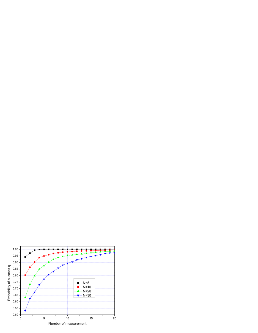
Figure 3: the probability of successful transfer within $j$ steps(measurements). The length of the spin chain is $N=5,10,20,30$, the interval of time $\tau_{i}$ is chosen to make $\eta_{i}$ the maximum.

As an example, in this section, We consider the equal nearest-neighbor coupling spin chain. The Hamiltonian of the chain($A_{1}+C+B$ or $A_{2}+C+B$) is

$$H=\frac{J}{2}\sum_{i=1}^{N-1}\{\sigma_{i}^{x}\sigma_{i+1}^{x}+\sigma_{i}^{y}\sigma_{i+1}^{y}\}.$$ (18)

The eigenvalues and eigenvectors have been solved exactly [4]. The probability of successful transfer within $j$ steps $\eta=\sum_{i=1}^{j}\eta_{i}(\tau_{i},N)$ is a function of number of spins $N$ , the interval time at the $i$th step $\tau_{i}$ and $j$. From Eq.(15), when $j=1$, and for a certain $N$, $\tau_{i}$ is chosen to make $\eta_{i}$ achieve its maximum, we get the maximal probability of successful transfer at the first step, as depicted in Fig.2. Because of the dispersion of the information along the chain, transfer is not perfect when the number of spins is larger than $3$, and the longer the spin chain, the less the maximal probability $\eta_{1}$. In Fig.3, $\tau_{i}$ is also chosen to make $\eta_{i}$ maximal. And this figure shows that when the number of measurement $j$ (number of decoding steps) increases, the probability of successful transfer $\eta$ approaches $1$ for all N.

The number of memories used is determined by the probability of successful transfer $\eta$ that we requires and the transfer ability of the spin chain. If we take $j$ steps to transfer the information to the memories, the time spent is $t_{j}=\sum_{i=1}^{j}\tau_{i}$, Burgarth [11] and  Giovannetti [10] have made a timescale estimation for $t_{j}$. In the decoding portion, if the decoding protocol is Time-reverse, the time spent on decoding is $t_{j}$, because all the $j$ steps should be finished to achieve the probability of successful transfer that we required. However, in our scheme, once the result of measurement of memories is $|1\rangle$, we can omit the following $(j-i)$ steps and complete the task of transfer. Therefore, we should use the average decoding time to measure the time for decoding.

$$\overline{T}=\sum_{i=1}^{j-1}\eta_{i}t_{i}+(1-\sum_{i=1}^{j-1}\eta_{i})t_{j}$$ (19)

The probability of successful transfer within $j-1$ steps is $\sum_{i=1}^{j-1}\eta_{i}$, so we have the probability $1-\sum_{i=1}^{j-1}\eta_{i}$ to go to the last decoding step. From Fig.2, the maximal probability of success is very large at the first step, i.e, when $N<25$, we have $\eta_{1}>0.5$. And from Fig.3, generally, $\eta_{i}$ is the decreasing function of $i$. So, we expect that $\overline{T}$ is obviously less than $t_{j}$. For example, when $N=10,J=20K\times\emph{k}_{B}$. Fifteen memories is needed to achieve the probability of successful transfer $\eta=0.99$. The time spent on the transfer portion is $t_{15}=0.37ns$, which is also the time spent on the decoding portion if we use the Time-reversed protocol. However, in our scheme, the average decoding time is $\overline{T}=3.02\times 10^{-2}ns$, which is only $\frac{1}{12}t_{15}$.

6 Conclusion

Because the information can be easily destroyed by measurement, conclusive transfer in a single spin chain was once thought to be unable [12]. Nevertheless, in our scheme, we successfully make it by using local memories storing the information and dividing the task into transfer portion and decoding portion. When the number of memories used and the decoding steps are infinite, our scheme can get perfect state transfer. Especially, our scheme is much better than Time-reversed protocol in some aspects. First, our scheme do not need another identical spin chain. Second, considering the timescale, the average decoding time in our scheme is much less than the Time-reversed protocol. Third, our scheme is conclusive transfer.

Acknowledgments:

The work was supported by the Fund of Chinese Academy of Sciences, the Education Ministry of China, and the National Natural Science Foundation of China under Grant No 10231050.

References

- [1] Nielsen M.A., Chuang I.L, Quantum Computation and information. Cambridge University, Cambrige, 2000.
- [2] S. Bose, Phys Rev Lett. 91(2003)207901.
- [3] C. Albanese, M. Christandl, N. Datta, and A. Ekert, Phys. Rev Lett. 93(2004)230502.
- [4] M. Christandl, N. Datta, T. C. Dorlas, A. Ekert, A. Kay, A. J. Landahl, Phys. Rev. A. 71(2005)032312
- [5] M. H. Yung, S. Bose, Phys. Rev. A.71(2005)032310
- [6] T. Shi, Y. Li, Z. Song, C. P. Sun, Phys. Rev. A 71(2005)032309
- [7] B. Chen, C.P.Sun, arXiv:quant-ph/0511246
- [8] Ying, Li. C. P. Sun, arXiv:quant-ph/0504175
- [9] A. Wojcik, T. Luczak, P. Kurzynski, A. Grudka, T. Gdala, M. Bednarska, Phys. Rev. A 72(2005)034303
- [10] V. Giovannetti, D. Burgarth, Phys. Rev. Lett 96(2006)030501
- [11] D. Burgarth, S. Bose, Phys. Rev. A 71(2005)052315
- [12] D. Burgarth, S. Bose, New J. Phys. 7(2005)135
- [13] A. D. Greentree, S. J. Devitt, L. C. L. Hollenberg. Phys. Rev. A 73(2006)032319
- [14] D. Burgarth, S. Bose, arXiv:quant-ph/0601047
- [15] G. D. Chiara, D. Rossini, R. Fazi, Phys. Rev. A 72(2005)012323
- [16] A. bayat, V. Karimipour, Phys. Rev. A 71(2005)042330
- [17] M. avellino, A.j.Fisher, arXiv:quant-ph/0603148
- [18] A. Serafini, M. Paternostro, S. Bose, arXiv:quant-ph/0511115
- [19] D. Burgarth, V. Giovannetti, S. Bose , arxiv:quant-ph/0410175