Single atom quantum walk with 1D optical superlattices

Abstract

A proposal for the implementation of quantum walks using cold atom technology is presented. It consists of one atom trapped in time varying optical superlattices. The required elements are presented in detail including the preparation procedure, the manipulation required for the quantum walk evolution and the final measurement. These procedures can be, in principle, implemented with present technology.

I Introduction

Ever since the idea of quantum walk was originally proposed in 1993 Aharonov , it has been understood as an interference phenomenon of quantum states Knight1 . Various implementations of quantum walks have been proposed employing atoms Dur , ions Ma or optics elements Knight1 . One proposal Dur which is particularly noteworthy proposes a way to perform quantum walks in optical lattices Jaksch04 , where cold atoms are utilized in the Mott insulator phase. One of the main challenges phased by these models is the decoherence of internal states in optical lattices during quantum walks.

Here we propose an alternative scheme for implementing quantum walks based on superlattices, which are formed by two optical lattices possessing different frequencies Kay . For that we employ a single atom trapped in superpositions of time modulated optical lattices in a one dimensional (1D) configuration. By employing two different superlattices, the state of the atom penetrates the left or right side through the optical potentials. The evolution is governed by direct tunneling of the atom between neighboring sites which can be made large enough to allow a significant number of steps within decoherence time. The preparation of the physical setup, the manipulation procedures and the subsequent measurements, is presented in detail in what follows.

In this paper, we begin with describing double well potentials in superlattices as a building block. In order to produce step operation in quantum walks, the state-dependent tunneling of the atom occurs into the direction of a lower optical barrier in the double well potential. By alternating two superlattices depending on the number of steps, we generate a standard Hadamard driven quantum walk. In addition, we consider the physical procedures that are needed to trap a single atom in a 1D optical lattice. We estimate the experimental parameters necessary for the realization of the quantum walk and the unitary errors in step operations due to uncontrolled laser properties. Finally, a measurement procedure is proposed that unambiguously distinguishes the quantum evolution from its classical counterpart.

II Quantum walks with superlattices

II.1 Superlattices as double wells

Let us consider a single atom that encodes a qubit in two possible states $0$ and $1$ characterized, e.g. by two different hyperfine levels. It is possible to trap this atom at a particular site within a 1D optical lattice that consists of two optical standing waves. A 1D optical lattice is given by

$$V(x) = V\cos{2\pi\over\lambda}x\,,$$ (1)

where $\lambda$ is the periodicity of the optical lattice used to trap cold atoms, viewed as dipoles, at its potential minima.

The superlattices are generated by interference of two optical lattices which have different frequencies. In particular, we consider an additional lattice with potential amplitude $V^{\prime}$, with double the wavelength of the first lattice. The resulting superlattice potential is given by

$$V(x) = V\cos{2\pi\over\lambda}x-V^{\prime}\cos\,{\pi\over\lambda}x,~{}~{}~{}~{}$$ (2)

as shown in Figure 1.

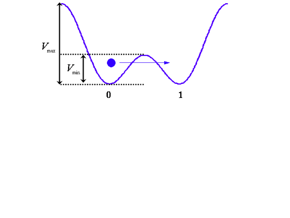
Figure 1: Tunneling of an atom in state $|0\rangle_{\rm int}$ appears from the left site to the right site in a double well ($V_{\rm max}=V+V^{\prime}$ and $V_{\rm min}=V-V^{\prime}$).

Our aim is to activate tunneling from one side to the other side depending on the internal state of the atom Kay . As shown in Figure 1, an initialized atom in the internal state $|0\rangle_{\rm int}$ is trapped in the left position $|0\rangle_{x}$ where subindexes “int” and “$x$” denote an internal state and a position state of the atom. In this section, we assume the ideal case such that the maximum amplitude of the superlattices $V_{\rm max}$ produces no tunneling for example between sites labeled 0 and $-1$ (to the left of the sites shown in Fig. 1) and the minimum amplitude $V_{\rm min}$ enables a tunneling between two positions in the double well. Thus, one can restrict between two sites where the tunneling interaction $J$ is activated by the superlattice

$$H=-J(a_{1}^{\dagger}a_{2}+a_{2}^{\dagger}a_{1}).$$ (3)

The time evolution operator is described by

$$U(t_{1},t_{0}) = \cos\big{(}{\textstyle{{1\over 2}}}J\Delta t\big{)}{\bf 1}+{\rm i}\,\sin\big{(}{\textstyle{{1\over 2}}}J\Delta t\big{)}\sigma_{x}\,,$$ (4)

where $\Delta t=t_{1}-t_{0}$ and $\sigma_{x}$ is one of the Pauli operators in the basis $|0\rangle_{x}$ and $|1\rangle_{x}$ that denote the two possible position states of the double well. In order to obtain perfect tunneling between two sites, a time $\Delta t=\pi/J$ is required during which the initial position state $|0\rangle_{x}$ becomes $|1\rangle_{x}$.

II.2 Quantum walks using 1D superlattices

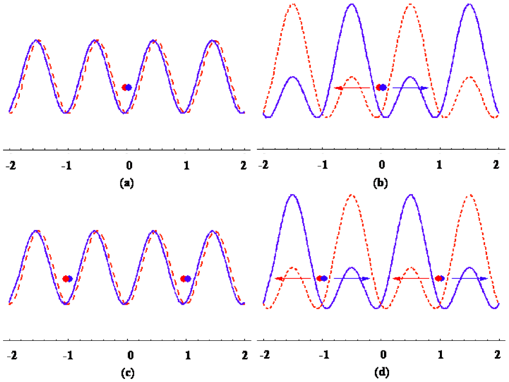
Figure 2: (a) The superposed atom is located at site $x=0$ of optical lattices. (b) By employing two superlattices the tunneling is activated depending on the internal state of the atom. (c) A Hadamard operation is performed in optical lattices. (d) The tunneling by alternating two superlattices occur among five sites at the second step of quantum walks.

We next demonstrate that quantum walks can be achieved by tunneling in two state-dependent super-lattices. In order to describe symmetric quantum walks Dur , we prepare an initialized atom in superposed state $|\psi_{0}\rangle={1\over\sqrt{2}}(|0\rangle_{\rm int}+{\rm i}|1\rangle_{\rm int})\otimes|0\rangle_{x}$. The subindex $n$ of state $|\psi_{n}\rangle$ indicates the number of steps. To implement a quantum walk we need to construct the step evolution operator Dur

$$S=\sum_{l=-\infty}^{\infty} (|0\rangle_{\rm int}\langle 0|\otimes|l+1\rangle_{x}\langle l|$$ (5)

$$+|1\rangle_{\rm int}\langle 1|\otimes|l-1\rangle_{x}\langle l|\big{)}.$$

As shown in Figure 2 (b) and (d), this is achieved by alternating between two different superlattice configurations. The first configuration of the superlattices is given by

$$V_{\rm odd}(x) = V_{i}\cos(2\pi x)+(-1)^{i}V^{\prime}_{i}\cos\,(\pi x),~{}~{}~{}~{}$$ (6)

where $i=0,1$ corresponds to the lattice that traps the $i$-th state of the atom. In the next step, the applied superlattices are given by

$$V_{\rm even}(x) = V_{i}\cos(2\pi x)-(-1)^{i}V^{\prime}_{i}\cos\,(\pi x).~{}~{}~{}~{}$$ (7)

As we see in Figure 2, the atom is located in even positions for even $n$ while it sits in odd positions for odd $n$. According to Eq. (4), alternating superlattices build two different step operators acting on the atom during the quantum walks as follows

$${S}_{\rm odd} = \sum_{l=-\infty}^{\infty}\big{(}|0\rangle_{\rm int}\langle 0|\otimes|2l+1\rangle_{x}\langle 2l|$$ (8)

$$~{}~{}~{}~{}~{}+|1\rangle_{\rm int}\langle 1|\otimes|2l-1\rangle_{x}\langle 2l|\big{)},~{}~{}~{}~{}~{}$$

$${S}_{\rm even} = \sum_{l=-\infty}^{\infty}\big{(}|0\rangle_{\rm int}\langle 0|\otimes|2l\rangle_{x}\langle 2l-1|$$ (9)

$$~{}~{}~{}~{}~{}+|1\rangle_{\rm int}\langle 1|\otimes|2l-2\rangle_{x}\langle 2l-1|\big{)}.~{}~{}~{}~{}~{}$$

Indeed, by applying these potentials in succession, two step operators perform one-directional state-dependent walks identically and the step operator $S$ can be implemented.

In order to generate a superposed internal state in every step, we introduce the Hadamard operation rev

$$H={1\over\sqrt{2}}\left(\begin{array}[]{cc}1&1\\ 1&-1\end{array}\right),$$ (12)

in the basis $|0\rangle_{\rm int}$ and $|1\rangle_{\rm int}$. When this operation is performed on all atoms in optical lattices, the internal states in each site evolve into superposition states. In terms of quantum optics, this Hadamard operator is decomposed into three Pauli operators which can be achieved by sequential $\pi/2$ laser pulses over all the sites (see Section IIIB in Ref. Dur ). Combined with the Hadamard operation between every step operator the standard Hadamard quantum walk is implemented. After performing $n$ steps, the final state is given by $|\psi_{n}\rangle=(SH)^{n}|\psi_{0}\rangle$.

We start to perform the Hadamard operation on the initialized state $|\psi_{0}\rangle$. After the first tunneling occurs during time $\Delta t=\pi/J_{\rm min}$, the state of the atom is described by

$$|\psi_{1}\rangle = {1\over\sqrt{2}}({\rm e}^{\rm i{\pi\over 4}}|0\rangle_{\rm int}\otimes|1\rangle_{x}+{\rm e}^{-\rm i{\pi\over 4}}|1\rangle_{\rm int}\otimes|-1\rangle_{x}).~{}~{}~{}~{}~{}$$ (13)

As a result, the state of the atom becomes an entangled state between the internal states and their positions. Then, we switch off the two additional lasers $V^{\prime}_{i}$ ($i=0,1$), which effectively turns off the tunneling between the two neighboring sites. If the Hadamard operation is applied on three sites, the atomic state is described in terms of both internal states and positions (see Figure 2 (c)).

To complete the second step of the quantum walk, we perform the step operation by the superlattice ${V}_{\rm even}(x)$ as shown in Figure 2 (d). Then, the atomic state after the second step of the walk equals

$$|\psi_{2}\rangle = {1\over 2}\big{(}|0\rangle_{\rm int}\otimes({\rm e}^{\rm i{\pi\over 4}}|2\rangle_{x}+{\rm e}^{-\rm i{\pi\over 4}}|0\rangle_{x})$$ (14)

$$\,+|1\rangle_{\rm int}\otimes({\rm e}^{\rm i{\pi\over 4}}|0\rangle_{x}-{\rm e}^{-\rm i{\pi\over 4}}|-2\rangle_{x})\big{)}.~{}~{}$$

Similarly, after the third step, the total state is

$$|\psi_{3}\rangle = {1\over 2\sqrt{2}}\big{(}|0\rangle_{\rm int}\otimes$$

$$\left[{\rm e}^{\rm i{\pi\over 4}}|3\rangle_{x}+({\rm e}^{\rm i{\pi\over 4}}+{\rm e}^{-\rm i{\pi\over 4}})|1\rangle_{x}-{\rm e}^{-\rm i{\pi\over 4}}|-1\rangle_{x}\right]$$

$$~{}~{}~{}+|1\rangle_{\rm int}\otimes$$

$$\left[{\rm e}^{\rm i{\pi\over 4}}|1\rangle_{x}-({\rm e}^{\rm i{\pi\over 4}}-{\rm e}^{-\rm i{\pi\over 4}})|-1\rangle_{x}+{\rm e}^{-\rm i{\pi\over 4}}|-3\rangle_{x}\right]\big{)}.$$

This demonstrates that the interference of each atomic state ($|0\rangle_{\rm int}$ and $|1\rangle_{\rm int}$) occurs respectively at position $x=1$ and $-1$ during quantum walks. Thus, the quantum walk is achieved by alternating superlattices, and produce the desired probability distribution of an atom over the sites of the 1D optical lattice.

III Physical Implementation

Let us now consider how to implement each of the elements necessary for realizing quantum walks in an 1D optical lattice. The required trapping of a single atom in the optical lattice can be achieved in a variety of ways. Subsequently, alternating superlattices are required to achieve state-dependent quantum walks. The realization of 1D and 2D superlattices have been recently demonstrated Sebby-Strabley ; Phillips . We analyze the amplitudes of the lasers necessary to generate the desired tunneling ratios. Furthermore, the condition is derived for performing the optical lattice modulations adiabatically to avoid heating the trapped atom. We investigate how robust the result of quantum walks is when imperfect tunneling is considered. Finally, we describe a measurement scheme that can distinguish the behavior of quantum walks from their corresponding classical counterpart.

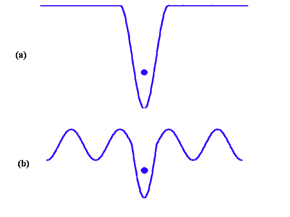
Figure 3: (a) A single atom is trapped in a position and (b) the trapping potential is reduced and a 1D optical lattice is employed.

III.1 Single atom trapping in 1D optical lattice

In order to trap a neutral atom, a simple method is to produce a deep harmonic potential. A well-focused laser beam builds a micro-trap (an optical tweezer trap) which can grab a single atom in an optical potential Pinkse ; Darquie . The schemes of trapping pointer atoms are also available to generate a single atom at a certain site Solano ; Kay06 . Alternatively, one can use the quantum Zeno effect by continuously fluorescent measurements to obtain a pointer atom Kay . When an optical lattice is applied across the trapping region, the atom can remain stable in a minimum of optical lattice (see Figure 3). Thus, to trap a single atom at a certain site within a 1D optical lattice seems experimentally feasible.

III.2 Laser amplitude regime

As we have seen, in order to perform step operation in the quantum walk one needs to control the laser amplitude corresponding to each atomic state. This will result to a tunneling coupling $J_{\sigma}$ that depends on the internal state, $\sigma$, of the atom. In particular, the tunneling couplings depend on the amplitude of the laser radiation, $V$, in the following way Scheel

$$J~{}(V)={E_{R}\over 2}\exp(-{\pi^{2}\over 4}\sqrt{V\over E_{R}})\left[\sqrt{V\over E_{R}}+\left({V\over E_{R}}\right)^{3/2}\right],~{}~{}$$ (16)

where $E_{R}$ is the recoil energy.

Hence, by selectively varying the amplitudes of the laser radiation at the in-between site regions it is possible to activate the tunneling interaction between the desired lattice sites. This is achieved by superlattices that give the spatial amplitude variation $V_{\rm max}=V_{i}+V^{\prime}_{i}$ and $V_{\rm min}=V_{i}-V^{\prime}_{i}$ ($i=0,1$). If the tunneling of the maximal potential $V_{\rm max}$ is much smaller than that of the minimal potential $V_{\rm min}$, the result of our quantum walk achieves the required outcome. Taking into account the two tunneling couplings $J_{\rm max}=J~{}(V_{\rm max})$ and $J_{\rm min}=J~{}(V_{\rm min})$, we demand that the ratio $J_{\rm max}/J_{\rm min}$ is close to zero. For instance, the amplitude of the first optical lattice $V_{0}$ in Eq. (1) can be taken to be approximately $25\,E_{R}$, i.e. the system is taken well into the Mott-insulating phase Mandel . When the second optical lattice with amplitude $V^{\prime}_{0}$ is applied, we consider $J_{\rm max}/J_{\rm min}$ as a function of $V^{\prime}_{0}$. As shown in Figure 4, when $V^{\prime}_{0}\approx 17.5\,E_{R}$, the ratio of two couplings can be maintained at a sufficiently small value (e.g. $J_{\rm max}/J_{\rm min}\approx 0.001$) to suppress undesired tunneling.

In addition, the superlattices must be switched on adiabatically. Typically, an atom in Mott-insulating optical lattices is trapped in a ground state. If we change optical potentials rapidly the atom can be kicked to an excited state or out of the optical potentials. Thus, adiabatic modulation from optical lattices to superlattices is required to avoid heating the trapped atom. For the experimentally achievable trapping frequency of $\omega_{\rm T}=30$kHz Mandel ; Jaksch98 a suitable time $\delta T\approx 33\mu s$ can be employed for the adiabatic evolution.

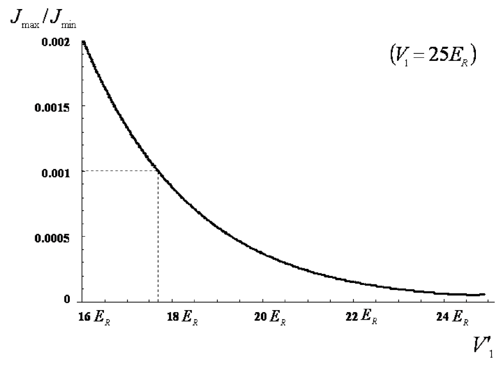
Figure 4: This demonstrates that more perfect tunneling is produced for fixed laser coupling $V_{1}$ when the second laser coupling $V^{\prime}_{1}$ becomes larger.

III.3 Study of errors

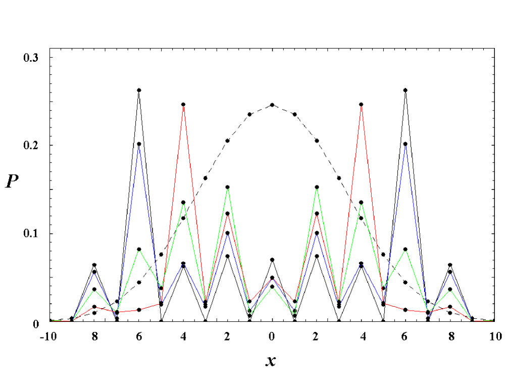
Figure 5: Probability distributions for $n=10$ without errors $\delta t_{0}=0$ (black) with errors $\delta t_{0}=0.2/J_{\rm min}$ (blue), $0.4/J_{\rm min}$ (green), and $0.6/J_{\rm min}$ (red). The dashed line shows the probability distribution for $n=10$ in a classical walk.

Here, sources of experimental errors are taken into account. In Ref. Dur , the decoherence of internal states is mainly considered because this reduces the quantum walk to its classical counterpart. The instability of laser beams (e.g. uncontrollable phase shifts) can influence the mobility of trapped atoms and cause imperfect manipulations during quantum walks. Nevertheless, we can restrict ourselves to less than two dozen steps in quantum walks, where the coherence of the internal states can be maintained.

To model these errors we consider an incomplete tunneling produced by the imperfect modulation of trapping potentials. In our setup, a major error can be produced by the fluctuation of the laser pulse time $\Delta t=\pi/J(V_{\text{min}})$. Taking into account this undesired effect, the unitary operation in Eq. (4) is no longer $\sigma_{x}$ during the tunneling procedure. When the tunneling by lowering optical potentials is not perfectly timed, then the atomic state becomes a superposition state in position during the tunneling. In this case, quantum walks cannot be described by the step operator $S$ in Eq. (5). Even though this defect does not cause the decoherence of internal states, it generates a different kind of quantum walk through odd and even steps. Shapira et al. Shapira investigated the case of similar unitary noises in the Hadamard operations during 1D quantum walks. They showed that the procedure with unitary noise evolves from quantum to classical walk distributions depending on the number of steps. Here we consider unitary errors in the step operations. A more controllable setup can vary the period of laser pulses in the Hadamard or step operation, thus generating different step operators and quantum coin tossing, which may be used for aperiodic quantum walks Ribeiro .

As shown in Figure 5, the error case demonstrates a leakage of probability distribution compared with perfect tunneling and also shows different aspects from the classical walks. When the period of the laser beam (with error $\delta t_{0}$) is described by $\Delta t=\pi/J_{\rm min}+\delta t_{0}$, the larger error value of the laser pulse time $\delta t$ generates a narrower dispersion of the atomic states (see color lines in Figure 5). Eventually, if $\delta t=\pi/J_{\rm min}$, the characteristic interference behavior of quantum walks does not appear due to the lack of a step operation in the procedure.

III.4 Measurement procedure

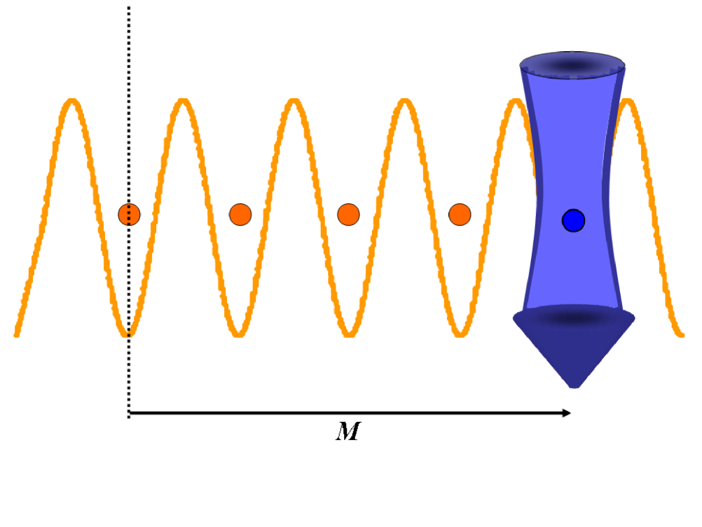
Figure 6: Fluorescence measurements by a short wavelength laser beam at distance $M$ to obtain a probability distribution.

In order to make sure that quantum walks have been performed, we need to evaluate the probability distribution at a certain lattice position. When we use relatively long-wavelength optical lattices, a single atom can be measured at a certain site at distance $M$ from the initial site by a well-focused laser beam using fluorescent measurements Roos (see Figure 6).

If we want to measure the atomic state in the $N$-th site away from the initial site, we shift the measurement laser to the distance $M=N\lambda$ ($\lambda$ is the wavelength of the trapping laser). Then, the laser pulse is applied continuously for a certain period. Here we can assume that the width of the focused laser beam sufficiently small enough not to disturb the other states in neighboring sites. By observing fluorescence histograms, the atomic state in the site can be measured Roos .

In this way one can distinguish between a quantum walk evolution and a classical one by detecting at which step, $n$, of the control procedure, population has been built at a site $N$. If one measures the atomic state over all sites in each step, the distribution of probabilities in a certain step shows the behavior characteristic of classical walks. Then, the probability at a specific site increases with respect to more steps due to the dispersion of the atomic state. However, if we only measure the atomic state at the end of the quantum walks, the occupation probability at the specific site fluctuates over the different number of total steps.

In Figure 7, we plot the probability at the same site in quantum walks with respect to the number of steps. The probability at the sixth site appears after the fifth step in both classical and quantum cases. While the value of probabilities gradually grow up in the classical case over lager $n$, the probabilities rapidly fluctuate in the quantum walk cases due to quantum coherence. For example, the probability at the tenth step ($n=10$) in perfect quantum walks reaches the highest peak, approximately 0.26, and drops to zero while it only increases monotonically from about 0.04 in the classical distribution. Therefore, we see that a reliable characterization of the evolution can be deduced within several steps of quantum walks.

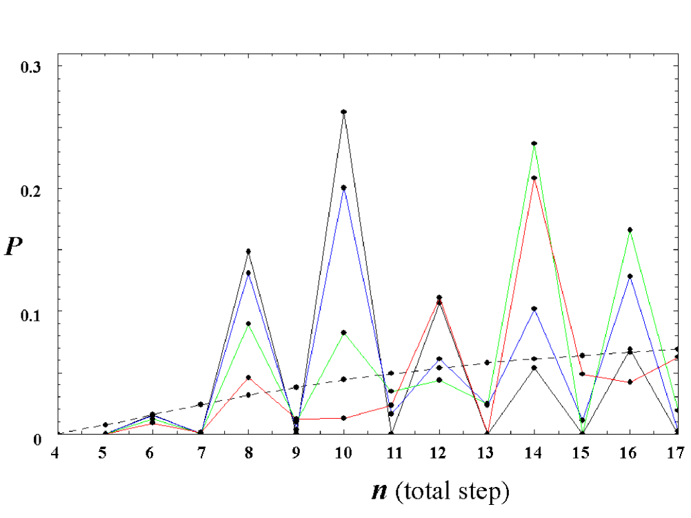
Figure 7: The plot shows that the probabilities of quantum walks (lined) at the sixth site ($N=6$) fluctuates between the fourth and seventeenth steps while that of classical walks (dashed) increases continuously. (errors with the same colors as shown in Figure 5).

IV Conclusion

In this article we have proposed a physical realization of a quantum walk with one atom manipulated within time varying optical lattices. A detailed study of the required elements is given and a study of the relevant errors is presented. The interaction coupling of the evolution is given by direct tunneling of an atom from one site to its neighbor which can be made significantly large. Imperfect tunneling generates unitary errors in quantum walks but it still shows quantum behaviors in probability distribution. Finally, we describe a feasible measurement approach which can distinguish the two different probability distributions of classical and quantum walks at a certain site. This gives the possibility to perform several algorithmic steps within the decoherence times of the system, typically taken to be of the order of a second Greiner .

V Acknowledgment

J. J. is supported by an IT Scholarship from the Ministry of Information and Communication, Republic of Korea and the Overseas Research Student Award Program. This work was also supported in part by the European Union Networks SCALA and CONQUEST and by the UK Engineering and Physical Sciences Research Council Interdisciplinary Research Collaboration on Quantum Information Processing.

References

- (1) Y. Aharonov, L. Davidovich, and N. Zagury, Phys. Rev. A 48, 1687 (1993).
- (2) P. L. Knight, E. Roldan, and J. E. Sipe, Phys. Rev. A 68, 020301(R) (2003); M. Hillery, J. Bergou, and E. Feldman, Phys. Rev. A 68, 032314 (2003); H. Jeong, M. Paternostro, and M. S. Kim, Phys. Rev. A 69, 012310 (2004); K. Eckert, J. Mompart, G. Birkl, and M. Lewenstein, Phys. Rev. A 72, 012327 (2005).
- (3) W. Dür, R. Raussendorf, V. M. Kendon, and H.-J. Briegel, Phys. Rev. A66, 052319 (2002).
- (4) Z.-Y. Ma and K. Burnett, M. B. d Arcy, and S. A. Gardiner, Phys. Rev. A 73, 013401 (2006); B. C. Sanders, S. D. Bartlett, B. Tregenna, and P. L. Knight, Phys. Rev. A 67, 042305 (2003); B. C. Travaglione and G. J. Milburn, Phys. Rev. A 65, 032310 (2002).
- (5) D. Jaksch, Contemp. Phys. 45, 367 (2004).
- (6) A. Kay and J. K. Pachos, New J. Phys. 6 126 (2004); quant-ph/0406073.
- (7) T. P. Spiller, W. J. Munro, S. D. Barrett, and P. Kok, Contemp. Phys. 46, 407 (2005) and references therein.
- (8) S. Peil, J. V. Porto, B. L. Tolra, J. M. Obrecht, B. E. King, M. Subbotin, S. L. Rolston, and W. D. Phillips, Phys. Rev. A 67, 051603(R) (2003).
- (9) J. Sebby-Strabley, M. Anderlini, P. S. Jessen, and J. V. Porto, Phys. Rev. A 73, 033605 (2006).
- (10) P. W. H. Pinkse, T. Fischer, P. Maunz, and G. Rempe, Nature 404, 365 (2000).
- (11) B. Darquie, M. P. A. Jones, J. Dingjan, J. Beugnon, S. Bergamini, Y. Sortais, G. Messin, A. Browaeys, and P. Grangier, Science 309, 454 (2005).
- (12) K. G. H. Vollbrecht, E. Solano, and J. I. Cirac, Phys. Rev. Lett. 93, 220502 (2004).
- (13) A. Kay, J. Pachos, and C. S. Adams, Phys. Rev. A 73, 022310 (2006).
- (14) S. Scheel, J. K. Pachos, E. A. Hinds, and P. L. Knight, Lect. Notes Phys. 689, 47 (2006); quant-ph/0403152.
- (15) O. Mandel, M. Greiner, A. Widera, T. Rom, T. W. Hänsch, and I. Bloch, Nature 425, 937 (2003).
- (16) D. Jaksch, C. Bruder, J. I. Cirac, C. W. Gardiner, and P. Zoller Phys. Rev. Lett. 81, 3108 (1998).
- (17) D. Shapira, O. Biham, A. J. Bracken, and M. Hackett, Phys. Rev. A 68, 062315 (2003).
- (18) P. Ribeiro, P. Milman, and R. Mosseri, Phys. Rev. Lett. 93, 190503 (2004).
- (19) C. F. Roos, M. Riebe, H. Häffner, W. Hänsel, J. Benhelm, G. P. T. Lancaster, C. Becher, F. Schmidt-Kaler, and R. Blatt, Science 304, 1478 (2004).
- (20) M. Greiner, O. Mandel, T. Esslinger, T. W. Hänsch, I. Bloch, Nature 415, 39 (2002).