Mass Detection with Nonlinear Nanomechanical Resonator

Abstract

Nanomechanical resonators having small mass, high resonance frequency and low damping rate are widely employed as mass detectors. We study the performances of such a detector when the resonator is driven into a region of nonlinear oscillations. We predict theoretically that in this region the system acts as a phase-sensitive mechanical amplifier. This behavior can be exploited to achieve noise squeezing in the output signal when homodyne detection is employed for readout. We show that mass sensitivity of the device in this region may exceed the upper bound imposed by thermomechanical noise upon the sensitivity when operating in the linear region. On the other hand, we show that the high mass sensitivity is accompanied by a slowing down of the response of the system to a change in the mass.

I Introduction

Nano-electro-mechanical systems (NEMS) serve in a variety of applications as sensors and actuators. Recent studies have demonstrated ultra-sensitive mass sensors based on NEMS Wachter and Thundat (1995); Lang et al. (1998); Hu et al. (2001); Ilic et al. (2000); Fritz et al. (2000); Ilic et al. (2001); Subramanian et al. (2002); Ilic et al. (2004a, b, 2005); Ekinci et al. (2004a); Ghatkesar et al. (2004); Ghatnekar-Nilsson et al. (2005). Such sensors promise a broad range of applications, from ultra-sensitive mass spectrometers that can be used to detect hazardous molecules, through biological applications at the level of a single DNA base-pair, to the study of fundamental questions such as the interaction of a single pair of molecules. In these devices mass detection is achieved by monitoring the resonance frequency $\omega_{0}$ of one of the modes of a nanomechanical resonator. The dependence of $\omega_{0}$ on the effective mass $m$ allows for sensitive detection of additional mass being adsorbed on the surfaces of the resonator. In such mass detectors the adsorbent molecules are anchored to the resonator surface either by Van der-Waals interaction, or by covalent bonds to linker molecules that are attached to the surface. Various analytes were used in those experiments, including alcohol and explosive gases, biomolecules, single cells, DNA molecules, and alkane chains. Currently, the smallest detectable mass change is $\delta m\simeq 0.4\times 10^{-21}\operatorname{kg}$ Ilic et al. (2004b), achieved by using a $4\operatorname{\mu m}$ long silicon beam with a resonance frequency $\omega_{0}/2\pi=10\operatorname{MHz}$, a quality factor $Q$ of about $2,500$, and total mass $m\simeq 5\times 10^{-16}\operatorname{kg}$. In a recent experiment Ilic et al. Ilic et al. (2005) succeeded to measure a single DNA molecule of about $1,600$ base pairs, which corresponds to $\delta m\simeq 1.6\times 10^{-21}\operatorname{kg}$, by using a silicon nitride cantilever, and employing an optical detection scheme.

In general, any detection scheme employed for monitoring the mass can be characterized by two important figures of merit. The first is the minimum detectable change in mass $\delta m$. This parameter is determined by the responsivity, which is defined as the derivative of the average output signal $\left\langle X\left(t\right)\right\rangle$ of the detector with respect to the mass $m$, the noise level, which is usually characterized by the spectral density of $X\left(t\right)$, and by the averaging time $\tau$ employed for measuring the output signal $X\left(t\right)$. The second figure of merit is the ring-down time $t_{\mathrm{RD}}$, which is a measure of the time width of the step in $X\left(t\right)$ due to a sudden change in $m$.

A number of factors affect the minimum detectable mass $\delta m$ and the ring-down time $t_{\mathrm{RD}}$ of mass detectors, based on nanomechanical resonators. Recent studies Ekinci et al. (2004b); Cleland (2005) have shown that if measurement noise is dominated by thermomechanical fluctuations the following hold

$$\frac{\delta m}{m}=2\left(\frac{2\pi}{Q\omega_{0}\tau}\frac{k_{B}T}{U_{0}}\right)^{1/2}\ ,$$ (1)

where $k_{B}T$ is the thermal energy, $U_{0}$ is the energy stored in the resonator, and $\tau$ is the measurement averaging time, and the ring-down time is given by

$$t_{\mathrm{RD}}=\frac{Q}{\omega_{0}}\ .$$ (2)

Eq. (1) indicates that nanomechanical resonators having small $m$ and high $\omega_{0}$ may allow high mass sensitivity (small $\delta m$). Further enhancement in the sensitivity can be achieved by increasing $Q$ however, this will be accompanied by an undesirable increase in the ring-down time, namely, slowing down the response of the system to changes in $m$. Moreover, Eq. (1) apparently suggests that unlimited reduction in $\delta m$ can be achieved by increasing $U_{0}$ by means of increasing the drive amplitude. Note however that Eq. (1), which was derived by assuming the case of linear response, is not applicable in the nonlinear region. Thus, in order to characterize the performances of the system when nonlinear oscillations are excited by an intense drive, one has to generalize the analysis by taking nonlinearity into account. From a more general point of view, such a generalization is interesting because it provides some insight onto the question of what is the range of applicability of the fluctuation-dissipation theorem for nonlinear systems Wang and Heinz (2002).

In the present paper we generalize Eqs. (1) and (2) and extend their range of applicability by taking into account nonlinearity in the response of the resonator to lowest order. Practically, characterizing the performances of nanomechanical mass detectors in the nonlinear region is important since in many cases, when a displacement detector with a sufficiently high sensitivity is not available, the oscillations of the system in the linear regime cannot be monitored, and consequently operation is possible only in the region of nonlinear oscillations. Another possibility for exploiting nonlinearity for enhancing mass sensitivity was recently studied theoretically by Cleland Cleland (2005), who has considered the case where the mechanical resonator is excited parametrically.

When nonlinearity is taken into account to lowest order the resonator’s dynamics can be described by the Duffing equation of motion Landau and Lifshits (1976). A Duffing resonator may exhibit bistability when driven by an external periodic force with amplitude $p$ exceeding some critical value $p_{c}$. Figure 1 below shows the calculated response vs. drive frequency $\omega_{p}$ of a Duffing resonator excited by a driving force with (b) sub-critical $p=p_{c}/2$ (c) critical $p=p_{c}$, and (d) over-critical $p=2p_{c}$ amplitude. The range of bistability in the $\left(\omega_{p},p\right)$ plane is seen in Fig. 1 (a). As was shown in Ref. Yurke and Buks (2005), high responsivity can be achieved when driving the resonator close to the edge of the bistability region Wiesenfeld and McNamara (1986); Dykman et al. (1994); Kromer et al. (2000); Savel’ev et al. (2005); Chan and C.Stambaugh (2006), where the slope of the response vs. frequency curve approaches infinity. Note however that in the same region of operation an undesirable slowing down occurs, namely $t_{\mathrm{RD}}$ can become much longer than its value in the linear region, which is given by Eq. (2).

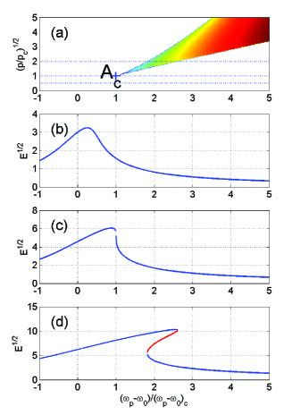
Figure 1: (Color online) Response of a driven Duffing resonator. Panel (a) shows the bistable region in the $\left(\omega_{p},p\right)$ plane. The response vs. frequency is shown in panel (b), (c) and (d) for sub-critical, critical, and over-critical driving force respectively.

The detector’s performances depend in general on the detection scheme which is being employed. Here we consider the case of a homodyne detection scheme Yurke and Buks (2005), where the output signal of a displacement detector monitoring the mechanical motion of the resonator is mixed with a local oscillator at the frequency of the driving force and with an adjustable phase $\phi_{\mathrm{LO}}$. In the nonlinear regime of operation the device acts as a phase sensitive intermodulation amplifier Almog et al. (2006a). Consequently, noise squeezing occurs in this regime, as was recently demonstrated experimentally in Ref. Almog et al. (2006b), namely, the spectral density of the output signal at the IF port of the mixer depends on $\phi_{\mathrm{LO}}$ periodically Rugar and Grutter (1991).

To optimize the operation of the system in the nonlinear region it is important to understand the role played by damping. In this region, in addition to linear damping, also nonlinear damping may affect the device performances. Our theoretical analysis Yurke and Buks (2005) shows that instability in a Duffing resonator is accessible only when the nonlinear damping is sufficiently small. Moreover, a fit between theory and experimental results allows extracting the nonlinear damping rate. By employing such a fit it was found in Ref. Zaitsev and Buks (2005) that nonlinear damping can play a significant role in the dynamics in the nonlinear region, and thus we take it into account in our analysis.

The paper is organized as follows. In section II the Hamiltonian of the driven Duffing resonator is introduced. The equations of motion of the system are derived in section III and linearized in section IV. The basins of attraction of the system are presented in section V. The ring-down time is estimated in section VI, whereas the case of homodyne detection is discussed in section VII. The calculation of the spectral density of the output signal of the homodyne detector, which is presented in section VIII, allows to calculate the minimum detectable mass in section IX. We conclude by comparing our findings with the linear case in section X.

II Hamiltonian

Consider a nonlinear mechanical resonator of mass $m$, resonance frequency $\omega_{0}$, damping rate $\gamma$, nonlinear Kerr constant $K$, and nonlinear damping rate $\gamma_{3}$. The resonator is driven by harmonic force at frequency $\omega_{p}$. The complex amplitude of the force $f$ is written as

$$f=-2im\omega_{p}x_{0}p^{1/2}e^{i\phi_{p}}\ ,$$ (3)

where $p$ is positive real, $\phi_{p}$ is real, and $x_{0}$ is give by

$$x_{0}=\sqrt{\frac{\hbar}{2m\omega_{0}}}\ .$$ (4)

The Hamiltonian of the system is given by Yurke and Buks (2005)

$$H=H_{1}+H_{a_{2}}+H_{a_{3}}+H_{c2}+H_{c3}\ ,$$ (5)

where $H_{1}$ is the Hamiltonian for the driven nonlinear resonator

$$H_{1} =\hbar\omega_{0}A^{\dagger}A+\frac{\hbar}{2}KA^{\dagger}A^{\dagger}AA$$

$$+\hbar p^{1/2}\left(ie^{i\left(\phi_{p}-\omega_{p}t\right)}A^{\dagger}-ie^{-i\left(\phi_{p}-\omega_{p}t\right)}A\right)\ .$$

The resonator’s creation and annihilation operators satisfy the following commutation relation

$$\left[A,A^{\dagger}\right]=AA^{\dagger}-A^{\dagger}A=1\ .$$ (7)

The Hamiltonians $H_{a2}$ and $H_{a3}$ associated with both baths are given by

$$H_{a2}=\int\mathrm{d}\omega\hbar\omega a_{2}^{\dagger}\left(\omega\right)a_{2}\left(\omega\right)\ ,$$ (8)

$$H_{a3}=\int\mathrm{d}\omega\hbar\omega a_{3}^{\dagger}\left(\omega\right)a_{3}\left(\omega\right)\ .$$ (9)

The Hamiltonian $H_{c2}$ linearly couples the bath modes $a_{2}\left(\omega\right)$ to the resonator mode $A$

$$H_{c2}=\hbar\sqrt{\frac{\gamma}{\pi}}\int\mathrm{d}\omega\left[e^{i\phi_{2}}A^{\dagger}a_{2}\left(\omega\right)+e^{-i\phi_{2}}a_{2}^{\dagger}\left(\omega\right)A\right]\ ,$$ (10)

whereas $H_{c3}$ describes two-phonon absorptive coupling of the resonator mode to the bath modes $a_{3}\left(\omega\right)$ in which two resonator phonons are destroyed for every bath phonon created

$$H_{c3}=\hbar\sqrt{\frac{\gamma_{3}}{\pi}}\int\mathrm{d}\omega\left[e^{i\phi_{3}}A^{\dagger}A^{\dagger}a_{3}(\omega)+e^{-i\phi_{3}}a_{3}^{\dagger}(\omega)AA\right]\ .$$ (11)

Both phase factors $\phi_{2}$ and $\phi_{3}$ are real. The bath modes are boson modes, satisfying the usual Bose commutation relations

$$[a_{n}(\omega),a_{n}^{\dagger}(\omega^{\prime})] =\delta\left(\omega-\omega^{\prime}\right)\ ,$$ (12)

$$\ [a_{n}(\omega),a_{n}(\omega^{\prime})] =0\ .$$ (13)

III Equations of Motion

We now generate the Heisenberg equations of motion according to

$$i\hbar\frac{dO}{dt}=\left[O,H\right]\ ,$$ (14)

where $O$ is an operator and $H$ is the total Hamiltonian

$$i\frac{\mathrm{d}A}{\mathrm{d}t} =\omega_{0}A+KA^{\dagger}AA+ip^{1/2}e^{i\phi_{p}}e^{-i\omega_{p}t}$$

$$+\sqrt{\frac{\gamma}{\pi}}e^{i\phi_{2}}\int\mathrm{d}\omega a_{2}\left(\omega\right)+2\sqrt{\frac{\gamma_{3}}{\pi}}e^{i\phi_{3}}A^{\dagger}\int\mathrm{d}\omega a_{3}(\omega)\ ,$$

$$\frac{\mathrm{d}a_{2}\left(\omega\right)}{\mathrm{d}t}=-i\omega a_{2}\left(\omega\right)-i\sqrt{\frac{\gamma}{\pi}}e^{-i\phi_{2}}A\ ,$$ (16)

$$\frac{\mathrm{d}a_{3}\left(\omega\right)}{\mathrm{d}t}=-i\omega a_{3}\left(\omega\right)-i\sqrt{\frac{\gamma_{3}}{2\pi}}e^{-i\phi_{3}}AA\ .$$ (17)

Using the standard method of Gardiner and Collett Gardiner and Collett (1985), and employing a transformation to a reference frame rotating at angular frequency $\omega_{p}$

$$A=Ce^{-i\omega_{p}t}\ ,$$ (18)

yield the following equation for the operator $C$

$$\frac{\mathrm{d}C}{\mathrm{d}t}+\Theta=F\left(t\right)\ ,$$ (19)

where

$$\Theta=\left[\gamma+i\left(\omega_{0}-\omega_{p}\right)+\left(iK+\gamma_{3}\right)C^{\dagger}C\right]C-p^{1/2}e^{i\phi_{p}}\ .$$ (20)

The noise term $F\left(t\right)$ is given by

$$F=-i\sqrt{2\gamma}e^{i\phi_{2}}a_{2}^{in}e^{i\omega_{p}t}-i2\sqrt{\gamma_{3}}e^{i\phi_{3}}C^{\dagger}a_{3}^{in}e^{2i\omega_{p}t}\ ,$$ (21)

where

$$a_{2}^{in}\left(t\right)=\frac{1}{\sqrt{2\pi}}\int\mathrm{d}\omega e^{-i\omega\left(t-t_{0}\right)}a_{2}\left(t_{0},\omega\right)\ ,$$ (22)

$$a_{3}^{in}\left(t\right)=\frac{1}{\sqrt{2\pi}}\int\mathrm{d}\omega e^{-i\omega\left(t-t_{0}\right)}a_{3}\left(t_{0},\omega\right)\ .$$ (23)

Note that in the noiseless case, namely when $F=0$, the equation of motion for the displacement $x$ of the vibrating mode can be written as

$$\frac{\mathrm{d}^{2}x}{\mathrm{d}t^{2}}+2\gamma\left[1+\frac{\gamma_{3}}{3\gamma}\left(\frac{x}{x_{0}}\right)^{2}\right]\frac{\mathrm{d}x}{\mathrm{d}t}+\omega_{0}^{2}\left[1+\frac{2K}{3\omega_{0}}\left(\frac{x}{x_{0}}\right)^{2}\right]x$$

$$=\frac{f}{m}e^{-i\omega_{p}t}+c.c.\ .$$

IV Linearization

Let $C=C_{m}+c$, where $C_{m}$ is a complex number for which

$$\Theta\left(C_{m},C_{m}^{\ast}\right)=0\ ,$$ (25)

namely, $C_{m}$ is a steady state solution of Eq. (19) for the noiseless case $F=0$. When the noise term $F$ can be considered as small, one can find an equation of motion for the fluctuation around $C_{m}$ by linearizing Eq. (19)

$$\frac{\mathrm{d}c}{\mathrm{d}t}+Wc+Vc^{\dagger}=F\ ,$$ (26)

where

$$W=\left.\frac{\partial\Theta}{\partial C}\right|_{C=C_{m}}=\gamma+i\left(\omega_{0}-\omega_{p}\right)+2\left(iK+\gamma_{3}\right)C_{m}^{\ast}C_{m}\ ,$$ (27)

and

$$V=\left.\frac{\partial\Theta}{\partial C^{\dagger}}\right|_{C=C_{m}}=\left(iK+\gamma_{3}\right)C_{m}^{2}\ .$$ (28)

IV.1 Mean-Field Solution

Using the notation

$$C_{m}=E^{1/2}e^{i\phi_{m}}\ ,$$ (29)

where $E$ is positive and $\phi_{m}\$is real, Eq. (25) reads

$$\left[\gamma+i\left(\omega_{0}-\omega_{p}\right)+\left(iK+\gamma_{3}\right)E\right]E^{1/2}e^{i\phi_{m}}=p^{1/2}e^{i\phi_{p}}\ .$$ (30)

Multiplying each side by its complex conjugate yields

$$\left[\left(\gamma+\gamma_{3}E\right)^{2}+\left(\omega_{0}-\omega_{p}+KE\right)^{2}\right]E=p\ .$$ (31)

Finding $E$ by solving the cubic polynomial Eq. (31) allows calculating $C_{m}$ using Eq. (30).

Taking the derivative of Eq. (31) with respect to the drive frequency $\omega_{p}$, one finds

$$\frac{\partial E}{\partial\omega_{p}}=\frac{2(\omega_{0}-\omega_{p}+KE)E}{\left|W\right|^{2}\left(1-\zeta^{2}\right)}\ ,$$ (32)

where

$$\zeta=\left|\frac{V}{W}\right|\ .$$ (33)

Similarly for the drive amplitude $p$

$$\frac{\partial E}{\partial p}=\frac{1}{\left|W\right|^{2}\left(1-\zeta^{2}\right)}\ .$$ (34)

Note that, as will be shown below, the value $\zeta=1$ occurs along the edge of the bistability region.

IV.2 The bifurcation point

At the bifurcation point, namely at the onset of bistability, the following holds

$$\frac{\partial\omega_{p}}{\partial E}=\frac{\partial^{2}\omega_{p}}{\partial E^{2}}=0\ .$$ (35)

Such a point occurs only if the nonlinear damping is sufficiently small Yurke and Buks (2005), namely, only when the following condition holds

$$|K|>\sqrt{3}\gamma_{3}\ .$$ (36)

At the bifurcation point the drive frequency and amplitude are given by

$$\left(\omega_{p}-\omega_{0}\right)_{c}=\gamma\frac{K}{|K|}\left[\frac{4\gamma_{3}|K|+\sqrt{3}\left(K^{2}+\gamma_{3}^{2}\right)}{K^{2}-3\gamma_{3}^{2}}\right]\ ,$$ (37)

$$p_{c}=\frac{8}{3\sqrt{3}}\frac{\gamma^{3}(K^{2}+\gamma_{3}^{2})}{\left(|K|-\sqrt{3}\gamma_{3}\right)^{3}}\ ,$$ (38)

and the resonator mode amplitude is

$$E_{c}=\frac{2\gamma}{\sqrt{3}\left(|K|-\sqrt{3}\gamma_{3}\right)}\ .$$ (39)

V Basins of Attraction

In the bistable region Eq. (25) has 3 different solutions, labeled as $C_{1},$ $C_{2}$ and $C_{3}$, where both stable solutions $C_{1}$ and $C_{3}$ are attractors, and the unstable solution $C_{2}$ is a saddle point. The bistable region $\Lambda$ in the plane of parameters $\left(\omega_{p},p\right)$ is seen in the colormap in Fig. 1 (a). The Kerr constant in this example is $K/\omega_{0}=0.001$, and the damping constants are $\gamma/\omega_{0}=0.02$, $\gamma_{3}=0.1K/\sqrt{3}$. The color in the bistable region $\Lambda$ indicates the difference $\left|C_{3}\right|^{2}-\left|C_{1}\right|^{2}$. The bifurcation point at $\omega_{p}-\omega_{0}=\left(\omega_{p}-\omega_{0}\right)_{c}$ and $p=p_{c}$ is labeled as $A_{c}$ in the figure.

Figure 2 (a) shows some flow lines obtained by integrating Eq. (19) numerically for the noiseless case $F=0$. The red and blue lines represent flow toward the attractors at $C_{1}$ and $C_{3}$ respectively. The green line is the seperatrix, namely the boundary between the basins of attraction of the attractors at $C_{1}$ and $C_{3}$. A closer view of the region near $C_{1}$ and $C_{2}$ is given in Fig. 2 (b). This figure shows also, an example of a random motion near the attractor at $C_{1}$ (seen as a cyan line). The line was obtained by numerically integrating Eq. (19) with a non vanishing fluctuating force $F$. The random walk demonstrates noise squeezing (to be further discussed below), where the fluctuations obtain their largest and smallest values along the directions of the local principle axes (see appendix).

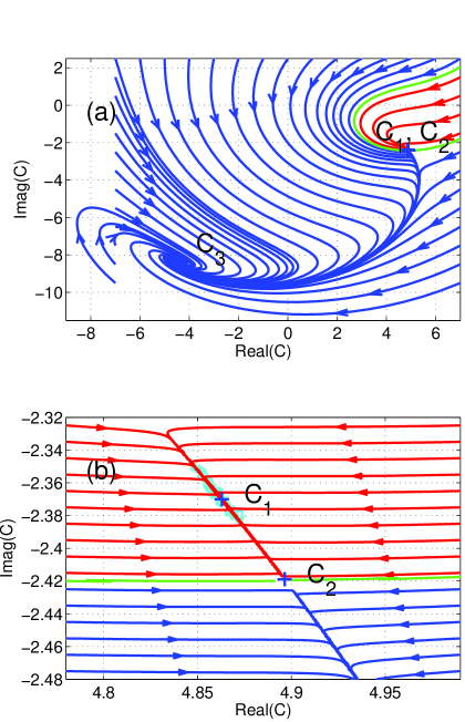
Figure 2: (Color online) Flow lines obtained by integrating Eq. (19) for the noiseless case $F=0$. The points $C_{1}$ and $C_{3}$ are attractors, and $C_{2}$ is a saddle point. The green line is the seperatrix, namely the boundary between the basins of attraction of both attractors. Panel (a) shows a wide view, whereas panel (b) shows a closer view of the region near $C_{1}$ and $C_{2}$. The cyan line near the attractor $C_{1}$ in panel (b) demonstrates random motion in the presence of noise.

VI Ring-Down Time

The solution of the equation of motion (26) was found in Ref. Yurke and Buks (2005)

$$c\left(t\right)=\int_{-\infty}^{\infty}\mathrm{d}t^{\prime}G\left(t-t^{\prime}\right)\Gamma\left(t^{\prime}\right)\ ,$$ (40)

where

$$\Gamma\left(t\right)=\frac{\mathrm{d}F\left(t\right)}{dt}+W^{\ast}F\left(t\right)-VF^{\dagger}\left(t\right)\ .$$ (41)

The propagator is given by

$$G\left(t\right)=u\left(t\right)\frac{e^{-\lambda_{0}t}-e^{\lambda_{1}t}}{\lambda_{1}-\lambda_{0}}\ ,$$ (42)

where $u(t)$ is the unit step function

$$u(t)=\left\{\begin{array}[c]{ll}1,&t>0\\ 1/2,&t=0\\ 0,&t<0\end{array}\right.\ ,$$ (43)

and $\lambda_{0}$ and $\lambda_{1}$ are the eigenvalues of the homogeneous equation, which satisfy

$$\lambda_{0}+\lambda_{1}=2W^{\prime}\ ,$$ (44)

$$\lambda_{0}\lambda_{1}=|W|^{2}-|V|^{2}\ ,$$ (45)

where $W^{\prime}$ is the real part of $W$. Thus one has

$$\lambda_{0,1}=W^{\prime}\left(1\pm\sqrt{1+\frac{|W|^{2}}{\left(W^{\prime}\right)^{2}}\left(\zeta^{2}-1\right)}\right)\ ,$$ (46)

or

$$\lambda_{0,1}=\gamma+2\gamma_{3}E\pm\sqrt{\left(K^{2}+\gamma_{3}^{2}\right)E^{2}-\left(\omega_{0}-\omega_{p}+2KE\right)^{2}}\ .$$ (47)

We chose to characterize the ring-down time scale as

$$t_{\mathrm{RD}}=\left(\lambda_{0}\lambda_{1}\right)^{-1/2}=\frac{1}{|W|\sqrt{1-\zeta^{2}}}\ .$$ (48)

Note that in the limit $\zeta\rightarrow 1$ slowing down occurs and $t_{\mathrm{RD}}\rightarrow\infty$. This limit corresponds to the case of operating the resonator near a jump point close to the edge of the bistability region.

VII Homodyne Detection

Consider the case where homodyne detection is employed for readout. In this case the output signal of a displacement detector monitoring the mechanical motion is mixed with a local oscillator at the same frequency as the frequency of the pump $\omega_{p}$ and having an adjustable phase $\phi_{\mathrm{LO}}$ ($\phi_{\mathrm{LO}}$ is real). The local oscillator is assumed to be noiseless. The output signal of the homodyne detector is proportional to

$$X_{\phi_{\mathrm{LO}}}\left(t\right)=e^{i\phi_{\mathrm{LO}}}C\left(t\right)+e^{-i\phi_{\mathrm{LO}}}C^{{\dagger}}\left(t\right)\ .$$ (49)

For the stationary case of a fixed mass $m$ the time varying signal $X_{\phi_{\mathrm{LO}}}\left(t\right)$ can be characterized by its average

$$X_{0}=\left\langle X_{\phi_{\mathrm{LO}}}\left(t\right)\right\rangle\ ,$$ (50)

and by its time auto-correlation function

$$K\left(t^{\prime}-t\right)=\left\langle\left[X_{\phi_{\mathrm{LO}}}\left(t\right)-X_{0}\right]\left[X_{\phi_{\mathrm{LO}}}\left(t^{\prime}\right)-X_{0}\right]\right\rangle\ .$$ (51)

The correlation function is expected to be an even function of $t^{\prime}-t$ with a maximum at $t^{\prime}-t=0$. The correlation time characterizes the width of that peak. Consider a measurement in which $X_{\phi_{\mathrm{LO}}}\left(t\right)$ is continuously monitored in the time interval $\left[0,\tau\right]$. Let $X_{\tau}$ be an estimator of the average value of $X_{\phi_{\mathrm{LO}}}\left(t\right)$

$$X_{\tau}=\frac{1}{\tau}\int_{0}^{\tau}\mathrm{d}t\ X_{\phi_{\mathrm{LO}}}\left(t\right)\ .$$ (52)

Clearly $X_{\tau}$ is unbiased, and its variance is given by

$$\left\langle\left(X_{\tau}-X_{0}\right)^{2}\right\rangle=\frac{1}{\tau^{2}}\int_{0}^{\tau}\mathrm{d}t\int_{0}^{\tau}\mathrm{d}t^{\prime}\ K\left(t^{\prime}-t\right)\ .$$ (53)

Assuming the case where the measurement time $\tau$ is much longer than the correlation time. For this case one can employ the approximation

$$\left\langle\left(X_{\tau}-X_{0}\right)^{2}\right\rangle=\frac{1}{\tau}\int_{-\infty}^{\infty}\mathrm{d}t\ K\left(t\right)\ ,$$ (54)

or in terms of the spectral density $P_{\phi_{\mathrm{LO}}}\left(\omega\right)$ of $X_{\phi_{\mathrm{LO}}}\left(t\right)$

$$\left\langle\left(X_{\tau}-X_{0}\right)^{2}\right\rangle=\frac{2\pi}{\tau}P_{\phi_{\mathrm{LO}}}\left(0\right)\ .$$ (55)

The responsivity $R$ of the detection scheme is defined as

$$R=\left|\frac{\partial X_{0}}{\partial m}\right|\ .$$ (56)

Using Eq. (55) one finds that the minimum detectable change in mass is given by

$$\delta m=R^{-1}\left(\frac{2\pi}{\tau}\right)^{1/2}P_{\phi_{\mathrm{LO}}}^{1/2}\left(0\right)\ .$$ (57)

Moreover, since $\omega_{0}$ is expected to be proportional to $m^{-1/2}$ one has

$$\frac{\delta m}{m}=\frac{2}{\omega_{0}}\left(\frac{2\pi}{\tau}\right)^{1/2}\left|\frac{\partial X_{0}}{\partial\omega_{0}}\right|^{-1}P_{\phi_{\mathrm{LO}}}^{1/2}\left(0\right)\ .$$ (58)

VIII Spectral Density

To calculate the spectral density $P_{\phi_{\mathrm{LO}}}\left(\omega\right)$ of $X_{\phi_{\mathrm{LO}}}\left(t\right)$ it is convenient to introduce the Fourier transform

$$c(t)=\frac{1}{\sqrt{2\pi}}\int_{-\infty}^{\infty}\mathrm{d}\omega c\left(\omega\right)e^{-i\omega t}\ ,$$ (59)

$$\Gamma(t)=\frac{1}{\sqrt{2\pi}}\int_{-\infty}^{\infty}\mathrm{d}\omega\Gamma\left(\omega\right)e^{-i\omega t}\ .$$ (60)

Assuming the bath modes are in thermal equilibrium, one finds

$$\left\langle F\left(\tau\right)\right\rangle=\left\langle F^{\dagger}\left(\tau\right)\right\rangle=0\ ,$$ (61)

$$\left\langle F\left(\tau\right)F\left(\tau^{\prime}\right)\right\rangle=\left\langle F^{\dagger}\left(\tau\right)F^{\dagger}\left(\tau^{\prime}\right)\right\rangle=0\ ,$$ (62)

$$\left\langle F\left(\tau\right)F^{\dagger}\left(\tau^{\prime}\right)\right\rangle=\left(\lambda_{0}+\lambda_{1}\right)\delta\left(\tau-\tau^{\prime}\right)\left\langle n_{\omega_{0}}\right\rangle\ ,$$ (63)

$$\left\langle F^{\dagger}\left(\tau\right)F\left(\tau^{\prime}\right)\right\rangle=\left(\lambda_{0}+\lambda_{1}\right)\delta\left(\tau-\tau^{\prime}\right)\left(\left\langle n_{\omega_{0}}\right\rangle+1\right)\ .$$ (64)

where

$$\left\langle n_{\omega}\right\rangle=\frac{1}{e^{\beta\hbar\omega}-1}\ ,$$ (65)

and $\beta=1/k_{B}T$.

In Ref. Yurke and Buks (2005); Buks and Yurke (2006) we have found that the following holds

$$c(\omega)=\frac{\Gamma(\omega)}{(-i\omega+\lambda_{0})(-i\omega+\lambda_{1})}\ .$$ (66)

where

$$\left\langle\Gamma(\omega)\right\rangle=\left\langle\Gamma^{{\dagger}}(\omega)\right\rangle=0\ ,$$ (67)

$$\left\langle\Gamma(\omega^{\prime})\Gamma(\omega)\right\rangle=\mathcal{N}_{1}\left(\omega\right)\delta\left(\omega+\omega^{\prime}\right)\ ,$$ (68)

$$\left\langle\Gamma^{{\dagger}}(\omega^{\prime})\Gamma^{{\dagger}}(\omega)\right\rangle=\mathcal{N}_{1}^{\ast}\left(\omega\right)\delta\left(\omega+\omega^{\prime}\right)\ ,$$ (69)

$$\left\langle\Gamma^{{\dagger}}(\omega^{\prime})\Gamma(\omega)\right\rangle+\left\langle\Gamma(\omega^{\prime})\Gamma^{{\dagger}}(\omega)\right\rangle=\mathcal{N}_{2}\left(\omega\right)\delta\left(\omega-\omega^{\prime}\right)\ ,$$ (70)

and

$$\mathcal{N}_{1}\left(\omega\right)=2W^{\prime}W^{\ast}V\coth\frac{\beta\hbar\omega_{0}}{2}\ ,$$ (71)

$$\mathcal{N}_{2}=2W^{\prime}\left(\left|W+i\omega\right|^{2}+\left|V\right|^{2}\right)\coth\frac{\beta\hbar\omega_{0}}{2}\ .$$ (72)

The frequency auto-correlation function of $X_{\phi_{\mathrm{LO}}}$ is related to the spectral density $P_{\phi_{\mathrm{LO}}}\left(\omega\right)$ by

$$\left\langle X_{\phi_{\mathrm{LO}}}(\omega^{\prime})X_{\phi_{\mathrm{LO}}}(\omega)\right\rangle=P_{\phi_{\mathrm{LO}}}\left(\omega\right)\delta\left(\omega-\omega^{\prime}\right)\ ,$$ (73)

thus one finds

$$P_{\phi_{\mathrm{LO}}}\left(\omega\right) =\frac{e^{2i\phi_{\mathrm{LO}}}\mathcal{N}_{1}\left(\omega\right)}{(i\omega+\lambda_{0})(i\omega+\lambda_{1})(-i\omega+\lambda_{0})(-i\omega+\lambda_{1})}$$

$$+\frac{e^{-2i\phi_{\mathrm{LO}}}\mathcal{N}_{1}^{\ast}\left(\omega\right)}{(-i\omega+\lambda_{0}^{\ast})(-i\omega+\lambda_{1}^{\ast})(i\omega+\lambda_{0}^{\ast})(i\omega+\lambda_{1}^{\ast})}$$

$$+\frac{\mathcal{N}_{2}\left(\omega\right)}{(i\omega+\lambda_{0}^{\ast})(i\omega+\lambda_{1}^{\ast})(-i\omega+\lambda_{0})(-i\omega+\lambda_{1})}\ ,$$

or in terms of the factors $W$ and $V$

$$P_{\phi_{\mathrm{LO}}}\left(\omega\right) =\frac{e^{2i\phi_{\mathrm{LO}}}W^{\ast}V+e^{-2i\phi_{\mathrm{LO}}}WV^{\ast}+\left|W+i\omega\right|^{2}+\left|V\right|^{2}}{(\omega-i\lambda_{0})(\omega+i\lambda_{0})(\omega-i\lambda_{1})(\omega+i\lambda_{1})}$$

$$\times 2W^{\prime}\coth\frac{\beta\hbar\omega}{2}\ .$$

(75)

VIII.0.1 Spectral Density at $\omega=0$

At frequency $\omega=0$ one finds

$$P_{\phi_{\mathrm{LO}}}\left(0\right)=\frac{1+2\zeta\cos\left(\phi_{\mathrm{LO}}-\phi_{0}\right)+\zeta^{2}}{\left(1-\zeta^{2}\right)^{2}}\frac{2W^{\prime}}{|W|^{2}}\coth\frac{\beta\hbar\omega_{0}}{2}\ ,$$ (76)

where the phase factor $\phi_{0}$ is defined in Eq. (97).

The largest value

$$\left[P_{\phi}\left(0\right)\right]_{\max}=\frac{1}{\left(1-\zeta\right)^{2}}\frac{2W^{\prime}}{|W|^{2}}\coth\frac{\beta\hbar\omega_{0}}{2}\ ,$$ (77)

is obtained when $\cos\left(\phi_{\mathrm{LO}}-\phi_{0}\right)=1$, and the smallest value

$$\left[P_{\phi}\left(0\right)\right]_{\min}=\frac{1}{\left(1+\zeta\right)^{2}}\frac{2W^{\prime}}{|W|^{2}}\coth\frac{\beta\hbar\omega_{0}}{2}\ ,$$ (78)

when $\cos\left(\phi_{\mathrm{LO}}-\phi_{0}\right)=-1$.

VIII.0.2 Integrated Spectral Density

The integral over all frequencies of the spectral density is easily calculated by employing the residue theorem

$$\frac{\int_{-\infty}^{\infty}P_{\phi_{\mathrm{LO}}}\left(\omega\right)\mathrm{d}\omega}{2\pi W^{\prime}\coth\frac{\beta\hbar\omega_{0}}{2}}=\frac{e^{2i\phi_{\mathrm{LO}}}W^{\ast}V+e^{-2i\phi_{\mathrm{LO}}}WV^{\ast}+2\left|W\right|^{2}}{\lambda_{0}\lambda_{1}(\lambda_{0}+\lambda_{1})}\ .$$

Using Eqs. (44) and (45) one finds

$$\frac{1}{2\pi}\int_{-\infty}^{\infty}P_{\phi_{\mathrm{LO}}}\left(\omega\right)\mathrm{d}\omega=\frac{1+\zeta\cos\left(\phi_{\mathrm{LO}}-\phi_{0}\right)}{1-\zeta^{2}}\coth\frac{\beta\hbar\omega_{0}}{2}\ .$$ (80)

Thus, the integrated spectral density peaks and deeps simultaneously with $P_{\phi_{\mathrm{LO}}}\left(0\right)$.

IX Minimum Detectable Mass

To evaluate $\delta m$ using Eq. (58) the responsivity factor $\partial X_{0}/\partial\omega_{0}$ has to be determined. Consider a small change $\delta\omega_{0}$ in the resonance frequency. Let $c_{m}$ be the resultant change in the steady state amplitude $C_{m}$ (here $c_{m}$ is considered as a c-number). Using Eqs. (25), (27), and (28) one finds

$$-iC_{m}\left(\delta\omega_{0}\right)=Wc_{m}+Vc_{m}^{\ast}\ .$$ (81)

Employing a coordinate transformation to the local principal axes (see appendix) and using Eq. (101) one finds

$$\left|C_{m}\right|e^{i\phi_{C}}\left(\delta\omega_{0}\right)=\left[\left(\left|W\right|+\left|V\right|\right)\xi+i\left(\left|W\right|-\left|V\right|\right)\eta\right]\ ,$$ (82)

where

$$\phi_{C}=\phi_{m}-\phi_{a}-\pi/2\ ,$$ (83)

and the phase factor $\phi_{m}$ is defined by Eq. (29). The inverse transformation Eq. (93) and Eq. (97) yield

$$c_{m}=e^{-i\phi_{0}}\left|\frac{C_{m}}{W}\right|\left(\frac{\cos\phi_{C}}{1+\zeta}+\frac{i\sin\phi_{C}}{1-\zeta}\right)\left(\delta\omega_{0}\right)\ ,$$ (84)

or

$$c_{m}=e^{-i\phi_{0}}\left|\frac{C_{m}}{W}\right|\frac{e^{i\phi_{C}}-\zeta e^{-i\phi_{C}}}{1-\zeta^{2}}\left(\delta\omega_{0}\right)\ .$$ (85)

The change in $X_{0}$ is given by $\delta X_{0}=e^{i\phi_{\mathrm{LO}}}c_{m}+e^{-i\phi_{\mathrm{LO}}}c_{m}^{\ast}$, thus one has

$$\frac{\partial X_{0}}{\partial\omega_{0}}=2\left|\frac{C_{m}}{W}\right|\operatorname{Re}\left(e^{i\left(\phi_{\mathrm{LO}}-\phi_{0}+\phi_{C}\right)}\frac{1-\zeta e^{-2i\phi_{C}}}{1-\zeta^{2}}\right)\ .$$ (86)

Finally, using Eqs. (58), (76), and (86), and assuming the case of high temperature

$$\beta\hbar\omega_{0}\ll 1\ ,$$ (87)

one finds

$$\frac{\delta m}{m}=2\left(\frac{2\pi}{Q_{\mathrm{eff}}\omega_{0}\tau}\frac{k_{B}T}{U_{0}}\right)^{1/2}g\left(\phi_{\mathrm{LO}}-\phi_{0}\right)\ ,$$ (88)

where $Q_{\mathrm{eff}}=\omega_{0}/W^{\prime}$ is the effective quality factor, the function $g$ is given by

$$g\left(\phi\right)=\frac{\left[1+2\zeta\cos\phi+\zeta^{2}\right]^{1/2}}{\left|\cos\left(\phi+\phi_{C}\right)-\zeta\cos\left(\phi-\phi_{C}\right)\right|}\ ,$$ (89)

and

$$U_{0}=\hbar\omega_{0}\left|C_{m}\right|^{2}\ .$$ (90)

In view of a comparison between Eq. (1) and Eq. (88) we refer to the case where $g<1$ as the case where the lower bound imposed upon the minimum detectable mass of a linear resonator is exceeded. The function $g\left(\phi_{\mathrm{LO}}-\phi_{0}\right)$ is plotted in Fig. (3) (a) for the case $\zeta=0.1$ and $\phi_{C}=0.5\pi$, and in Fig. (3) (b) for the case $\zeta=0.99$ and $\phi_{C}=0.5\pi$. For both cases values of $g$ below unity are obtained in some range of $\phi_{\mathrm{LO}}$. Figure (3) (c) shows the minimum value of the function $g\left(\phi_{\mathrm{LO}}-\phi_{0}\right)$ vs. $\phi_{C}$ for 3 different values of $\zeta$. In general $0.5\leq g_{\min}\leq 1$ for all values of $\phi_{C}$ and $\zeta$, whereas, the lowest value $g_{\min}=0.5$ is obtained in the limit $\zeta\rightarrow 1$. This limit corresponds to the case of operating close to a jump point, namely close to the edge of the bistability region.

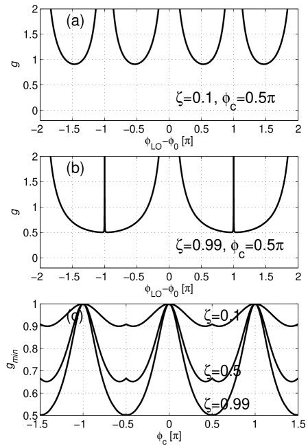
Figure 3: The function $g$. Panel (a) shows $g\left(\phi_{\mathrm{LO}}-\phi_{0}\right)$ for the case $\zeta=0.1$ and $\phi_{C}=0.5\pi$, and panel (b) for the case $\zeta=0.99$ and $\phi_{C}=0.5\pi$. Panel (c) shows the minimum value of the function $g\left(\phi_{\mathrm{LO}}-\phi_{0}\right)$ vs. $\phi_{C}$ for different values of $\zeta$.

X Conclusions

In the present paper we analyze the performances of a nanomechanical mass detector. Both Kerr nonlinearity and nonlinear damping are taken into account to lowest order. The lower bound imposed upon the minimum detectable mass due to thermomechanical noise is generalized for the present case. The lowest detectable mass is obtained when the resonator is driven close to a jump point near the edge of the bistability region. However, in the same region slowing-down occurs in the response of the detector to a change in the mass (see Eq. (48)), limiting thus the detection speed. In general, for a given application the operating point can be chosen to optimally balance between the different requirements on the sensitivity and response time.

Appendix A Principal Axes

Consider an expansion of the function $\Theta$ near a complex number $Z$

$$\Theta\left(Z+z,Z^{\ast}+z^{\ast}\right)=\Theta_{0}+Wz+Vz^{\ast}+O\left(\left|z\right|^{2}\right)\ ,$$ (91)

where $\Theta_{0}=\Theta_{0}\left(Z,Z^{\ast}\right)$, and $W$ and $V$ are given by Eqs. (27) and (28) respectively.

The transformation

$$\left(\begin{array}[c]{c}\xi\\ \eta\end{array}\right)=\frac{1}{2}\left(\begin{array}[c]{cc}e^{i\phi}&e^{-i\phi}\\ -ie^{i\phi}&ie^{-i\phi}\end{array}\right)\left(\begin{array}[c]{c}z\\ z^{\ast}\end{array}\right)\ ,$$ (92)

represents axes rotation with angle $\phi$ ($\phi$ is real). The inverse transformation is given by

$$\left(\begin{array}[c]{c}z\\ z^{\ast}\end{array}\right)=\left(\begin{array}[c]{cc}e^{-i\phi}&ie^{-i\phi}\\ e^{i\phi}&-ie^{i\phi}\end{array}\right)\left(\begin{array}[c]{c}\xi\\ \eta\end{array}\right)\ .$$ (93)

Using this notation one finds

$$Wz+Vz^{\ast}=R_{\xi}\xi+R_{\eta}\eta\ ,$$ (94)

where

$$R_{\xi} =We^{-i\phi}+Ve^{i\phi}\ ,$$ (95)

$$R_{\eta} =i\left(We^{-i\phi}-Ve^{i\phi}\right)\ .$$ (96)

Principle axes are obtained by choosing $\phi=\phi_{0}$ where

$$e^{2i\phi_{0}}=\frac{WV^{\ast}}{\left|WV\right|}\ .$$ (97)

Thus, using the notation

$$\left(\frac{WV}{\left|WV\right|}\right)^{1/2}=e^{i\phi_{a}}\ ,$$ (98)

one finds that in the reference frame of the principle axes the following hold

$$R_{\xi} =e^{i\phi_{a}}\left(\left|W\right|+\left|V\right|\right)\ ,$$ (99)

$$R_{\eta} =ie^{i\phi_{a}}\left(\left|W\right|-\left|V\right|\right)\ ,$$ (100)

and

$$Wz+Vz^{\ast}=e^{i\phi_{a}}\left[\left(\left|W\right|+\left|V\right|\right)\xi+i\left(\left|W\right|-\left|V\right|\right)\eta\right]\ .$$ (101)

References

• Wachter and Thundat (1995) E. A. Wachter and T. Thundat, Rev. Sci. Instrum. 66, 3662 (1995).
• Lang et al. (1998) H. P. Lang, , R. Berger, , C. Andreoli, , J. Brugger, M. Despont, P. Vettiger, C. Gerber, et al., Appl. Phys. Lett. 72, 383 (1998).
• Hu et al. (2001) Z. Y. Hu, T. Thundat, and R. J. Warmack, J. Appl. Phys. 90, 427 (2001).
• Ilic et al. (2000) B. Ilic, D. Czaplewski, H. G. Craighead, P. Neuzil, C. Campagnolo, and C. Batt, Appl. Phys. Lett. 77, 450 (2000).
• Fritz et al. (2000) J. Fritz, M. K. Baller, H. P. Lang, H. Rothuizen, P. Vettiger, E. Meyer, H. J. Guntherodt, C. Gerber, and J. K. Gimzewski, Science 288, 316 (2000).
• Ilic et al. (2001) B. Ilic, D. Czaplewski, M. Zalalutdinov, H. G. Craighead, P. Neuzil, C. Campagnolo, and C. Batt, J. Vac. Sci. Technol. B 19, 2825 (2001).
• Subramanian et al. (2002) A. Subramanian, P. I. Oden, S. J. Kennel, K. B. Jacobson, R. J. Warmack, T. Thundat, and M. J. Doktycz, Appl. Phys. Lett. 81, 385 (2002).
• Ilic et al. (2004a) B. Ilic, L. Yang, and H. G. Craighead, Appl. Phys. Lett. 85, 2604 (2004a).
• Ilic et al. (2004b) B. Ilic, H. G. Craighead, S. Krylov, W. Senarante, C. Ober, , and P. Neuzil, J. Appl. Phys. 95, 3694 (2004b).
• Ilic et al. (2005) B. Ilic, Y. Yang, K. Aubin, R. Reichenbach, S. Krylov, and H. G. Craighead, Nano Lett. 5, 925 (2005).
• Ekinci et al. (2004a) K. L. Ekinci, X. M. H. H, and M. L. Roukes, Appl. Phys. Lett. 84, 4469 (2004a).
• Ghatkesar et al. (2004) M. K. Ghatkesar, V. Barwich, T. Braun, A. H. Bredekamp, U. Drechsler, M. Despont, H. P. Lang, M. Hegner, and C. Gerber, Proc. IEEE Sensors 2004, 1060 (2004).
• Ghatnekar-Nilsson et al. (2005) S. Ghatnekar-Nilsson, E. Forsen, G. Abadal, J. Verd, F. Campabadal, F. Perez-Murano, J. Esteve, N. Barniol, A. Boisen, and L. Montelius, Nanotechnology 16, 98 (2005).
• Ekinci et al. (2004b) K. L. Ekinci, Y. T. Yang, and M. L. Roukes, J. Appl. Phys. 95, 2682 (2004b).
• Cleland (2005) A. N. Cleland, New J. Phys. 7, 235 (2005).
• Wang and Heinz (2002) E. Wang and U. Heinz, Phys. Rev. D 66, 025008 (2002).
• Landau and Lifshits (1976) L. Landau and E. Lifshits, Mechanics (Oxford, New York, 1976).
• Yurke and Buks (2005) B. Yurke and E. Buks, arXiv:quant-ph/0505018 v1 pp. 1–9 (2005).
• Wiesenfeld and McNamara (1986) K. Wiesenfeld and B. McNamara, Phys. Rev. A 33, 629 (1986).
• Dykman et al. (1994) M. Dykman, D. Luchinsky, R. Mannella, P. McClintock, N. Stein, and N. Stocks, Phys. Rev. E 49, 1198 (1994).
• Kromer et al. (2000) H. Kromer, A. Erbe, A. Tilke, S. Manus, and R. Blick, Europhys. Lett. 50, 101 (2000).
• Savel’ev et al. (2005) S. Savel’ev, A. L. Rakhmanov, and F. Nori, Phys. Rev. E 72, 056136 (2005).
• Chan and C.Stambaugh (2006) H. B. Chan and C.Stambaugh, arXiv:cond-mat/0603037 (2006).
• Almog et al. (2006a) R. Almog, S. Zaitsev, O. Shtempluck, and E. Buks, Appl. Phys. Lett. 88, 213509 (2006a).
• Almog et al. (2006b) R. Almog, S. Zaitsev, O. Shtempluck, and E. Buks, arXiv: cond-mat/0607055 (2006b).
• Rugar and Grutter (1991) D. Rugar and P. Grutter, Phys. Rev. Lett. 67, 699 (1991).
• Zaitsev and Buks (2005) S. Zaitsev and E. Buks, arXiv: cond-mat/0503130 (2005).
• Gardiner and Collett (1985) C. W. Gardiner and M. J. Collett, Phys. Rev. A 31, 3761 (1985).
• Buks and Yurke (2006) E. Buks and B. Yurke, Phys. Rev. A 73, 023815 (2006).