Body-assisted van der Waals interaction between two atoms

Abstract

Using fourth-order perturbation theory, a general formula for the van der Waals potential of two neutral, unpolarized, ground-state atoms in the presence of an arbitrary arrangement of dispersing and absorbing magnetodielectric bodies is derived. The theory is applied to two atoms in bulk material and in front of a planar multilayer system, with special emphasis on the cases of a perfectly reflecting plate and a semi-infinite half space. It is demonstrated that the enhancement and reduction of the two-atom interaction due to the presence of a perfectly reflecting plate can be understood, at least in the nonretarded limit, by using the method of image charges. For the semi-infinite half space, both analytical and numerical results are presented.

I Introduction

The dispersive interaction between two neutral, unpolarized, ground-state atoms—commonly known as the van der Waals (vdW) interaction—may be regarded, in the nonretarded limit, i.e., for small interatomic separations, as the mutual interaction of the fluctuating electric dipole moments of the atoms in the ground state. It was first calculated in this limit by London using perturbation theory, the leading-order result being an attractive potential proportional to $r^{-6}$, where $r$ denotes the interatomic separation lon . In the retarded limit, i.e., for large interatomic separations, the interaction is due to the ground-state fluctuations of both the atomic dipole moments and the electromagnetic far field. This was first demonstrated by Casimir and Polder, who identified the vdW interaction as the position-dependent shift of the system’s ground-state energy due to the coupling between the atoms and the electromagnetic field c-p . Using a normal-mode expansion of the electromagnetic field and calculating the energy shift in leading-order perturbation theory, they generalized the (nonretarded) London potential to arbitrary distances between the two atoms, where in particular in the retarded limit the potential was found to vary as $r^{-7}$.

The theory has been extended in many respects, and various factors affecting the vdW interaction have been studied. Based on a calculation of photon scattering amplitudes, Feinberg and Sucher extended the theory to magnetically polarizable atoms feinberg . They found that the vdW interaction of two magnetically polarizable atoms is again attractive, while for two atoms of opposed type—one magnetically and one electrically polarizable—a repulsive vdW force may be observed. Later on, it was demonstrated that in the case of two atoms of opposed type the nonretarded potential is proportional to $r^{-4}$, in contrast to the $r^{-6}$-dependence of the nonretarded potential of equal-type atoms Farina02 . The Feinberg-Sucher result was extended to particles exhibiting crossed polarizabilities eli . Further studies have also included the cases of one pass1 or both atoms p-t3 ; shr being excited, leading to potentials that vary as $r^{-6}$ and $r^{-2}$ in the nonretarded and retarded limits, respectively. Thermal photons present for any nonzero temperature have been shown to lead, in the retarded limit, to a change of the vdW potential of two ground-state atoms from a $r^{-7}$- to a $r^{-6}$-dependence as soon as the interatomic separation exceeds the wavelength of the dominant photons nin ; wen ; gdk ; bar . Modifications of the vdW interaction due to external fields have been shown to lead to a potential varying as $r^{-3}$ in the nonretarded limit when the applied field is unidirectional mil . Generalizations of the vdW interaction to the three- Axilrod43 ; Aub60 ; Cirone96 ; pass2 and $N$-atom case p-t1 ; p-t2 were addressed first in the nonretarded limit and later for arbitrary interatomic separations, where the potentials were seen to depend on the relative positions of the atoms in a rather complicated way.

Van der Waals interactions play an important role in the understanding of many phenomena—mostly in the field of surface science, such as surface tension Ninham97 ; Bostroem01 , adhesion Rabinowicz65 , and capillarity Rowlinson02 , but also in chemical physics, such as colloidal interactions Ninham97 ; Bostroem01b and stability Russel89 . However, application of the theoretical results to these phenomena requires taking into account the influence of media on the atom-atom interaction. An expression for the vdW interaction of two ground-state atoms in the presence of dielectric media was first obtained by Mahanty and Ninham based on a semiclassical approach Mahanty72 ; mah ; mah1976 , and was applied to the case of two atoms placed between two planar, perfectly conducting plates mah . The situation of two atoms between two perfectly conducting plates was later reconsidered taking into account finite temperature effects bos . Other scenarios such as two atoms placed within a planar dielectric three-layer geometry mar or two anisotropic molecules in front of a dielectric half space or within a planar dielectric cavity have also been studied Cho .

In this paper we present an exact derivation of a very general formula for the vdW potential of two ground-state atoms in the presence of an arbitrary arrangement of dispersing and absorbing magnetodielectric bodies. Based on macroscopic quantum electrodynamics in linearly, locally and causally responding media, and starting from the multipolar coupling Hamiltonian for the atom–field interaction in electric-dipole approximation, we calculate the vdW potential in leading, fourth-order perturbation theory. We then apply the general result to the cases that the two atoms are placed (i) within bulk material and (ii) in front of a planar magnetodielectric multilayer system.

The paper is organized as follows. In Sec. II the atom–field interaction Hamiltonian in its multipolar coupling form is presented. The derivation of the general formula for the vdW potential is given in Sec. III, and Sec. IV is devoted to the applications mentioned, where a detailed analytical as well as numerical analysis is given. Finally, the paper ends with a summary and conclusions in Sec. V.

II Multipolar-coupling Hamiltonian

The Hamiltonian for a system consisting of nonrelativistic charged particles $\alpha$ (each particle having charge $q_{\alpha}$, mass $m_{\alpha}$, position $\hat{\mathbf{r}}_{\alpha}$, and canonically conjugate momentum $\hat{\mathbf{p}}_{\alpha}$) interacting with the electromagnetic field in the presence of dispersing and absorbing magnetodielectric bodies is given by Knoll01 ; Ho03

$$\hat{H}= \sum_{\lambda=e,m}\int\mathrm{d}^{3}r\int_{0}^{\infty}\mathrm{d}\omega\,\hbar\omega\,\hat{\mathbf{f}}_{\lambda}^{\dagger}(\mathbf{r},\omega)\cdot\hat{\mathbf{f}}_{\lambda}(\mathbf{r},\omega)$$

$$+\sum_{\alpha}\frac{1}{2m_{\alpha}}\Bigl{[}\hat{\mathbf{p}}_{\alpha}-q_{\alpha}\hat{\mathbf{A}}(\hat{\mathbf{r}}_{\alpha})\Bigr{]}^{2}+{\textstyle\frac{1}{2}}\int\mathrm{d}^{3}r\,\hat{\rho}_{\mathrm{p}}(\mathbf{r})\hat{\varphi}_{\mathrm{p}}(\mathbf{r})$$

$$+\int\mathrm{d}^{3}r\,\hat{\rho}_{\mathrm{p}}(\mathbf{r})\hat{\varphi}(\mathbf{r}),$$ (1)

where

$$\hat{\rho}_{\mathrm{p}}(\mathbf{r})=\sum_{\alpha}q_{\alpha}\delta(\mathbf{r}-\hat{\mathbf{r}}_{\alpha})$$ (2)

and

$$\hat{\varphi}_{\mathrm{p}}(\mathbf{r})=\int\mathrm{d}^{3}{r}^{\prime}\,\frac{\hat{\rho}_{\mathrm{p}}(\mathbf{r}^{\prime})}{4\pi\varepsilon_{0}|\mathbf{r}-\mathbf{r}^{\prime}|}$$ (3)

are the charge density and scalar potential of the particles, respectively. The Bosonic fields $\hat{\mathbf{f}}_{\lambda}(\mathbf{r},\omega)$ and $\hat{\mathbf{f}}_{\lambda}^{\dagger}(\mathbf{r},\omega)$ are the canonically conjugate variables that describe the combined system of the electromagnetic field and the (inhomogeneous) magnetodielectric medium, including the dissipative system responsible for absorption,

$$\Bigl{[}\hat{f}_{\lambda i}(\mathbf{r},\omega),\hat{f}^{\dagger}_{\lambda^{\prime}i^{\prime}}(\mathbf{r}^{\prime},\omega^{\prime})\Bigr{]}=\delta_{\lambda\lambda^{\prime}}\delta_{ii^{\prime}}\delta(\mathbf{r}-\mathbf{r}^{\prime})\delta(\omega-\omega^{\prime}),$$ (4)

$$\Bigl{[}\hat{f}_{\lambda i}(\mathbf{r},\omega),\hat{f}_{\lambda^{\prime}i^{\prime}}(\mathbf{r}^{\prime},\omega^{\prime})\Bigr{]}=0,$$ (5)

where $\lambda$ $\!=$ $\!e$ ($\lambda$ $\!=$ $\!m$) refers to the electric (magnetic) excitations. The vector potential $\hat{\mathbf{A}}({\mathbf{r}})$ and the scalar potential $\hat{\varphi}({\mathbf{r}})$ of the medium-assisted electromagnetic field can in Coulomb gauge be expressed in terms of the dynamical variables $\hat{\mathbf{f}}_{\lambda}(\mathbf{r},\omega)$ and $\hat{\mathbf{f}}_{\lambda}^{\dagger}(\mathbf{r},\omega)$ as

$$\hat{\mathbf{A}}(\mathbf{r})=\int_{0}^{\infty}\mathrm{d}\omega\,(i\omega)^{-1}{\underline{\hat{\mathbf{E}}}}{}^{\perp}(\mathbf{r},\omega)+\mathrm{H.c.},$$ (6)

$$\bm{\nabla}\hat{\varphi}(\mathbf{r})=-\int_{0}^{\infty}\mathrm{d}\omega\,{\underline{\hat{\mathbf{E}}}}{}^{\parallel}(\mathbf{r},\omega)+\mathrm{H.c.},$$ (7)

with

$$\underline{\hat{\mathbf{E}}}(\mathbf{r},\omega)=\sum_{\lambda=e,m}\int\mathrm{d}^{3}r^{\prime}\,\bm{G}_{\lambda}(\mathbf{r},\mathbf{r}^{\prime},\omega)\cdot\hat{\mathbf{f}}_{\lambda}(\mathbf{r}^{\prime},\omega),$$ (8)

where

$$\bm{G}_{e}(\mathbf{r},\mathbf{r}^{\prime},\omega)=i\,\frac{\omega^{2}}{c^{2}}\sqrt{\frac{\hbar}{\pi\varepsilon_{0}}\,\mathrm{Im}\,\varepsilon(\mathbf{r}^{\prime},\omega)}\,\bm{G}(\mathbf{r},\mathbf{r}^{\prime},\omega),$$ (9)

$$\bm{G}_{m}({\mathbf{r}},{\mathbf{r}}{}^{\prime},\omega)=-i\,\frac{\omega}{c}\,\bm{G}(\mathbf{r},\mathbf{r}^{\prime},\omega)\!\times\!\!\overleftarrow{\bm{\nabla}}_{\!\!\mathbf{r}^{\prime}}\sqrt{-\frac{\hbar}{\pi\varepsilon_{0}}\,\mathrm{Im}\,\kappa(\mathbf{r}^{\prime},\omega)},$$ (10)

$\bigl{[}\bm{G}(\mathbf{r},\mathbf{r}^{\prime},\omega)\!\times\!\overleftarrow{\bm{\nabla}}_{\!\!\mathbf{r}^{\prime}}\bigr{]}_{ij}$ $\!=$ $\!\epsilon_{jkl}\partial^{\prime}_{l}G_{ik}(\mathbf{r},\mathbf{r}^{\prime},\omega)$, and $\perp$ ($\parallel$) denotes transverse (longitudinal) vector fields. In Eqs. (9) and (10), $\bm{G}(\mathbf{r},\mathbf{r}^{\prime},\omega)$ is the classical Green tensor obeying the equation

$$\biggl{[}\bm{\nabla}\times\kappa(\mathbf{r},\omega)\bm{\nabla}\times-\frac{\omega^{2}}{c^{2}}\,\varepsilon(\mathbf{r},\omega)\biggr{]}\bm{G}(\mathbf{r},\mathbf{r}^{\prime},\omega)=\bm{\delta}(\mathbf{r}-\mathbf{r}^{\prime})$$ (11)

together with the boundary condition at infinity. All relevant characteristics of the macroscopic bodies enter the theory via the space- and frequency-dependent complex permittivity $\varepsilon({\mathbf{r}},\omega)$ and permeability $\mu({\mathbf{r}},\omega)$ $\!=$ $\!\kappa^{-1}(\mathbf{r},\omega)$, with the real and imaginary parts of $\varepsilon({\mathbf{r}},\omega)$ and $\kappa(\mathbf{r},\omega)$ satisfying the Kramers–Kronig relations. Note that the Green tensor obeys the useful properties Knoll01

$$\bm{G}^{\ast}(\mathbf{r},\mathbf{r}^{\prime},\omega)=\bm{G}(\mathbf{r},\mathbf{r}^{\prime},-\omega^{\ast}),$$ (12)

$$\bm{G}(\mathbf{r},\mathbf{r}^{\prime},\omega)=\bm{G}^{\top}(\mathbf{r}^{\prime},\mathbf{r},\omega),$$ (13)

$$\sum_{\lambda=e,m}\int\mathrm{d}^{3}s\,\bm{G}_{\lambda}(\mathbf{r},\mathbf{s},\omega)\cdot\bm{G}^{+}_{\lambda}(\mathbf{r}^{\prime},\mathbf{s},\omega)$$

$$\hskip 21.52771pt=\frac{\hbar\mu_{0}}{\pi}\,\omega^{2}\mathrm{Im}\,\bm{G}(\mathbf{r},\mathbf{r}^{\prime},\omega).$$ (14)

If the charged particles constitute a system of neutral atoms and/or molecules (briefly referred to as atoms in the following) labelled by $A$, $\sum_{\alpha\in A}q_{\alpha}$ $\!=$ $\!0$, then it is convenient to employ the Hamiltonian in the multipolar-coupling form, which can be obtained from the minimal-coupling form (II) via a Power–Zienau transformation

$$\hat{U}=\exp\biggl{[}\frac{i}{\hbar}\int\mathrm{d}^{3}r\,\sum_{A}\hat{\mathbf{P}}_{A}(\mathbf{r})\cdot\hat{\mathbf{A}}(\mathbf{r})\biggr{]},$$ (15)

where the polarization of atom $A$ is given by

$$\hat{\mathbf{P}}_{A}(\mathbf{r})=\sum_{\alpha\in A}q_{\alpha}\hat{\bar{\mathbf{r}}}_{\alpha}\int_{0}^{1}\mathrm{d}\lambda\,\delta(\mathbf{r}-\hat{\mathbf{r}}_{A}-\lambda\hat{\bar{\mathbf{r}}}_{\alpha}),$$ (16)

with

$$\hat{\bar{\mathbf{r}}}_{\alpha}=\hat{\mathbf{r}}_{\alpha}-\hat{\mathbf{r}}_{A}$$ (17)

denoting the particle coordinates relative to the center of mass

$$\hat{\mathbf{r}}_{A}=\sum_{\alpha\in A}\frac{m_{\alpha}}{m_{A}}\,\hat{\mathbf{r}}_{\alpha}$$ (18)

of atom $A$ ($m_{A}$ $\!=$ $\!\sum_{\alpha\in A}m_{\alpha}$). We assume that all the atoms are (i) essentially at rest, $m_{\alpha}/m_{A}$ $\!\to$ $\!0$, (ii) small compared to the wavelength of the relevant field components, $\hat{\bar{\mathbf{r}}}_{\alpha}$ $\!\to$ $\!\hat{\mathbf{r}}_{A}$, and (iii) well separated from each other,

$$\int\mathrm{d}^{3}r\,\hat{\mathbf{P}}_{A}(\mathbf{r})\cdot\hat{\mathbf{P}}_{B}(\mathbf{r})=\delta_{AB}\int\mathrm{d}^{3}r\,\hat{\mathbf{P}}^{2}_{A}(\mathbf{r}).$$ (19)

Under these assumptions, the Hamiltonian in the multipolar coupling scheme can be obtained from Eqs. (II) and (15) in complete analogy to the procedure outlined in Ref. Buhmann04 , resulting in

$$\hat{H}=\hat{H}_{\mathrm{F}}+\sum_{A}\hat{H}_{A}+\sum_{A}\hat{H}_{A\mathrm{F}},$$ (20)

where

$$\hat{H}_{\mathrm{F}}=\sum_{\lambda=e,m}\int\mathrm{d}^{3}r\,\int_{0}^{\infty}\mathrm{d}\omega\,\hbar\omega\,\hat{\mathbf{f}}_{\lambda}{\!{}^{\dagger}}(\mathbf{r},\omega)\cdot\hat{\mathbf{f}}_{\lambda}(\mathbf{r},\omega),$$ (21)

$$\hat{H}_{A}=\sum_{\alpha\in A}\frac{\hat{\mathbf{p}}_{\alpha}{\!{}^{2}}}{2m_{\alpha}}+\frac{1}{2\varepsilon_{0}}\int\mathrm{d}^{3}r\,\hat{\mathbf{P}}_{A}^{2}(\mathbf{r}),$$ (22)

$$\hat{H}_{A\mathrm{F}}=-\hat{\mathbf{d}}_{A}\cdot\hat{\mathbf{E}}(\hat{\mathbf{r}}_{A})\!+\!\sum_{\alpha\in A}\frac{q_{\alpha}}{2m_{\alpha}}\hat{\bar{\mathbf{p}}}_{\alpha}\cdot[\hat{\bar{\mathbf{r}}}_{\alpha}\times\hat{\mathbf{B}}(\hat{\mathbf{r}}_{A})]$$

$$\hskip 30.1388pt+\sum_{\alpha\in A}\frac{q_{\alpha}^{2}}{8m_{\alpha}}\bigl{[}\hat{\bar{\mathbf{r}}}_{\alpha}\times\hat{\mathbf{B}}(\hat{\mathbf{r}}_{A})\bigr{]}^{2}.$$ (23)

In Eq. (II),

$$\hat{\mathbf{d}}_{A}=\sum_{\alpha\in A}q_{\alpha}\hat{\bar{\mathbf{r}}}_{\alpha}=\sum_{\alpha\in A}q_{\alpha}\hat{\mathbf{r}}_{\alpha}$$ (24)

is the electric dipole moment of atom $A$, and the electric and induction fields are given by

$$\hat{\mathbf{E}}(\mathbf{r})=\int_{0}^{\infty}\mathrm{d}\omega\,\underline{\hat{\mathbf{E}}}(\mathbf{r},\omega)+\mathrm{H.c.},$$ (25)

with $\underline{\hat{\mathbf{E}}}(\mathbf{r},\omega)$ from Eq. (8), and

$$\hat{\mathbf{B}}(\mathbf{r})=\int_{0}^{\infty}\mathrm{d}\omega\,\underline{\hat{\mathbf{B}}}(\mathbf{r},\omega)+\mathrm{H.c.},$$ (26)

$$\underline{\hat{\mathbf{B}}}(\mathbf{r},\omega)=(i\omega)^{-1}\bm{\nabla}\times\underline{\hat{\mathbf{E}}}(\mathbf{r},\omega).$$ (27)

Note that in the multipolar-coupling scheme $\hat{\mathbf{E}}(\mathbf{r})$ has the physical meaning of a displacement field w.r.t. the polarization of the atoms. Finally, in the case of atoms which are not magnetically polarizable, we may omit the second and third terms in Eq. (II) so that Eq. (II) reduces to the well-known electric-dipole term

$$\hat{H}_{A\mathrm{F}}=-\hat{\mathbf{d}}_{A}\cdot\hat{\mathbf{E}}(\hat{\mathbf{r}}_{A}).$$ (28)

III The van der Waals potential

Let us consider two neutral, ground-state atoms $A$ and $B$ at given positions $\mathbf{r}_{A}$ and $\mathbf{r}_{B}$ in the presence of arbitrarily shaped magnetodielectric bodies. Denoting by $|n_{A(B)}\rangle$ the (unperturbed) energy eigenstates of atom $A(B)$, we may represent the atomic Hamiltonian $H_{A(B)}$, Eq. (22), in the form

$$\hat{H}_{A(B)}=\sum_{n}E^{n}_{A(B)}|n_{A(B)}\rangle\langle n_{A(B)}|.$$ (29)

Restricting our attention to the electric-dipole approximation, the interaction Hamiltonian $\hat{H}_{A(B)\mathrm{F}}$ reads, according to Eq. (28) [$\hat{\mathbf{r}}_{A(B)}\mapsto\mathbf{r}_{A(B)}$],

$$\hat{H}_{A(B)\mathrm{F}}=\\ -\sum_{n}\sum_{m}|n_{A(B)}\rangle\langle m_{A(B)}|\mathbf{d}_{A(B)}^{nm}\cdot\hat{\mathbf{E}}(\mathbf{r}_{A(B)}),$$ (30)

where ${\mathbf{d}}_{A(B)}^{nm}$ $\!=$ $\!\langle n_{A(B)}|\hat{\mathbf{d}}_{A(B)}|m_{A(B)}\rangle$, and $\hat{\mathbf{E}}(\mathbf{r})$ is given by Eq. (25) together with Eq. (8). Further, let $|\{0\}\rangle$, $|1^{(\alpha)}\rangle$, and $|1^{(\beta)},1^{(\gamma)}\rangle$ be the vacuum, single-, and two-quantum excited states of the combined system consisting of the electromagnetic field and the bodies, respectively,

$${\hat{f}}_{\lambda i}(\mathbf{r},\omega)|\{0\}\rangle=0,$$ (31)

$$\hat{f}_{\lambda_{\alpha}i_{\alpha}}^{\dagger}(\mathbf{r_{\alpha}},\omega_{\alpha})|\{0\}\rangle\equiv|1^{(\alpha)}\rangle,$$ (32)

$${\textstyle\frac{1}{\sqrt{2}}}\,\hat{f}_{\lambda_{\beta}i_{\beta}}^{\dagger}(\mathbf{r_{\beta}},\omega_{\beta})\hat{f}_{\lambda_{\gamma}i_{\gamma}}^{\dagger}(\mathbf{r_{\gamma}},\omega_{\gamma})|\{0\}\rangle\equiv|1^{(\beta)},1^{(\gamma)}\rangle$$ (33)

[the corresponding single- und two-excitation energies are respectively $\hbar\omega_{\alpha}$ and $\hbar(\omega_{\beta}+\omega_{\gamma})$].

Following Casimir’s and Polder’s approach c-p (see also Ref. Craig84 ), we identify the two-atom vdW interaction with the position-dependent shift of the ground-state energy $\Delta E_{AB}$ calculated in leading-order perturbation theory according to

$$\Delta E_{AB}=-\sideset{}{{}^{\prime}}{\sum}_{I,II,III}\frac{\langle 0|\hat{H}_{A\mathrm{F}}\!+\!\hat{H}_{B\mathrm{F}}|III\rangle\langle III|\hat{H}_{A\mathrm{F}}\!+\!\hat{H}_{B\mathrm{F}}|II\rangle}{(E_{I}-E_{0})}$$

$$\hskip 43.05542pt\times\frac{\langle II|\hat{H}_{A\mathrm{F}}\!+\!\hat{H}_{B\mathrm{F}}|I\rangle\langle I|\hat{H}_{A\mathrm{F}}\!+\!\hat{H}_{B\mathrm{F}}|0\rangle}{(E_{II}-E_{0})(E_{III}-E_{0})}\,,$$ (34)

where the primed sum indicates that only intermediate states $|I\rangle$, $|II\rangle$, and $|III\rangle$ other than the (unperturbed) ground state of the overall system,

$$|0\rangle=|0_{A}\rangle|0_{B}\rangle|\{0\}\rangle,$$ (35)

are included in the summations. Note that the summations include position and frequency integrals.

From Eq. (30), by considering only two-atom virtual processes, it can be inferred that the intermediate states $|I\rangle$ and $|III\rangle$ have one of the atoms excited and one body-assisted field excitation present, while the intermediate states $|II\rangle$ can be of three types: (i) both atoms in the ground state with two field excitations present, (ii) both atoms excited with no field excitation present, and (iii) both atoms excited with two field excitations present. All possible intermediate states together with the respective energy denominators are listed in Tab. 2 in App. A.

Let us consider, e.g., case (1) in this table. Substituting the corresponding matrix elements (A)–(A) as given in App. A into Eq. (III), we derive the contribution $\Delta E_{AB(1)}$ to the two-atom energy shift $\Delta E_{AB}$ to be

$$\Delta E_{AB(1)}=-\frac{1}{2\hbar^{3}}\sum_{n,m}\,\sum_{i_{1},i_{2},i_{3},i_{4}}\sum_{\lambda_{1},\lambda_{2},\lambda_{3},\lambda_{4}}\Biggl{[}\prod_{j=1}^{4}\int\mathrm{d}^{3}r_{j}\int_{0}^{\infty}\mathrm{d}\omega_{j}\Biggr{]}\,\frac{1}{D_{nm}(\omega_{1},\omega_{2},\omega_{3},\omega_{4})}$$

$$\times\Big{\{}\big{[}\mathbf{d}_{A}^{n0}\!\cdot\!\bm{G}_{\lambda_{1}}^{\ast}(\mathbf{r}_{A},\mathbf{r}_{1},\omega_{1})\big{]}_{i_{1}}\big{[}\mathbf{d}_{A}^{0n}\!\cdot\!\bm{G}_{\lambda_{3}}^{\ast}(\mathbf{r}_{A},\mathbf{r}_{3},\omega_{3})\big{]}_{i_{3}}\big{[}\mathbf{d}_{B}^{m0}\!\cdot\!\bm{G}_{\lambda_{3}}(\mathbf{r}_{B},\mathbf{r}_{3},\omega_{3})\big{]}_{i_{3}}\big{[}\mathbf{d}_{B}^{0m}\!\cdot\!\bm{G}_{\lambda_{4}}(\mathbf{r}_{B},\mathbf{r}_{4},\omega_{4})\big{]}_{i_{4}}\delta^{(12)}\delta^{(24)}$$

$$\quad+\big{[}\mathbf{d}_{A}^{n0}\!\cdot\!\bm{G}_{\lambda_{1}}^{\ast}(\mathbf{r}_{A},\mathbf{r}_{1},\omega_{1})\big{]}_{i_{1}}\big{[}\mathbf{d}_{A}^{0n}\!\cdot\!\bm{G}_{\lambda_{3}}^{\ast}(\mathbf{r}_{A},\mathbf{r}_{3},\omega_{3})\big{]}_{i_{3}}\big{[}\mathbf{d}_{B}^{m0}\!\cdot\!\bm{G}_{\lambda_{2}}(\mathbf{r}_{B},\mathbf{r}_{2},\omega_{2})\big{]}_{i_{2}}\big{[}\mathbf{d}_{B}^{0m}\!\cdot\!\bm{G}_{\lambda_{4}}(\mathbf{r}_{B},\mathbf{r}_{4},\omega_{4})\big{]}_{i_{4}}\delta^{(12)}\delta^{(34)}$$

$$\quad+\big{[}\mathbf{d}_{A}^{n0}\!\cdot\!\bm{G}_{\lambda_{1}}^{\ast}(\mathbf{r}_{A},\mathbf{r}_{1},\omega_{1})\big{]}_{i_{1}}\big{[}\mathbf{d}_{A}^{0n}\!\cdot\!\bm{G}_{\lambda_{2}}^{\ast}(\mathbf{r}_{A},\mathbf{r}_{2},\omega_{2})\big{]}_{i_{2}}\big{[}\mathbf{d}_{B}^{m0}\!\cdot\!\bm{G}_{\lambda_{2}}(\mathbf{r}_{B},\mathbf{r}_{2},\omega_{2})\big{]}_{i_{2}}\big{[}\mathbf{d}_{B}^{0m}\!\cdot\!\bm{G}_{\lambda_{4}}(\mathbf{r}_{B},\mathbf{r}_{4},\omega_{4})\big{]}_{i_{4}}\delta^{(13)}\delta^{(34)}$$

$$\quad+\big{[}\mathbf{d}_{A}^{n0}\!\cdot\!\bm{G}_{\lambda_{1}}^{\ast}(\mathbf{r}_{A},\mathbf{r}_{1},\omega_{1})\big{]}_{i_{1}}\big{[}\mathbf{d}_{A}^{0n}\!\cdot\!\bm{G}_{\lambda_{2}}^{\ast}(\mathbf{r}_{A},\mathbf{r}_{2},\omega_{2})\big{]}_{i_{2}}\big{[}\mathbf{d}_{B}^{m0}\!\cdot\!\bm{G}_{\lambda_{3}}(\mathbf{r}_{B},\mathbf{r}_{3},\omega_{3})\big{]}_{i_{3}}\big{[}\mathbf{d}_{B}^{0m}\!\cdot\!\bm{G}_{\lambda_{4}}(\mathbf{r}_{B},\mathbf{r}_{4},\omega_{4})\big{]}_{i_{4}}\delta^{(13)}\delta^{(24)}\Big{\}},$$ (36)

where

$$\delta^{(\alpha\beta)}=\delta_{i_{\alpha}i_{\beta}}\delta_{\lambda_{\alpha}\lambda_{\beta}}\delta(\mathbf{r}_{\alpha}-\mathbf{r}_{\beta})\delta(\omega_{\alpha}-\omega_{\beta})$$ (37)

and

$$D_{nm}(\omega_{1},\omega_{2},\omega_{3},\omega_{4})=(\omega_{A}^{n}\!+\!\omega_{1})(\omega_{2}\!+\!\omega_{3})(\omega_{B}^{m}\!+\!\omega_{4})$$ (38)

[$\omega_{A(B)}^{n}$ $\!=$ $\!(E^{n}_{A(B)}$ $\!-$ $\!E^{0}_{A(B)})/\hbar$]. Recalling Eq. (II), we may simplify Eq. (III) to

$$\Delta E_{AB(1)}=-\frac{\mu_{0}^{2}}{\hbar\pi^{2}}\sum_{n,m}\int_{0}^{\infty}{\mathrm{d}}\omega\int_{0}^{\infty}{\mathrm{d}}\omega^{\prime}\,\omega^{2}\omega^{\prime 2}$$

$$\quad\times\bigg{(}\frac{1}{D_{\mathrm{i}}}+\frac{1}{D_{\mathrm{ii}}}\bigg{)}\big{[}{\mathbf{d}}_{A}^{0n}\!\cdot\!{\rm Im}\bm{G}({{\mathbf{r}}_{A}},{{\mathbf{r}}_{B}},\omega)\!\cdot\!{\mathbf{d}}_{B}^{0m}\big{]}$$

$$\quad\hskip 43.05542pt\times\big{[}{\mathbf{d}}_{A}^{0n}\!\cdot\!{\rm Im}\bm{G}({{\mathbf{r}}_{A}},{{\mathbf{r}}_{B}},\omega^{\prime})\!\cdot\!{\mathbf{d}}_{B}^{0m}\big{]},$$ (39)

where $D_{\mathrm{i}}$ and $D_{\mathrm{ii}}$ are respectively the first and the second denominators in Tab. 2, and without loss of generality we have assumed that the matrix elements of the electric-dipole operators are real.

The contributions $\Delta E_{AB(k)}$ to $\Delta E_{AB}$ which correspond to the cases (2)–(10) in Table 2 in App. A can be calculated analogously. It turns out that they differ from Eq. (III) only in the energy denominators. It is not difficult to prove that summation of the energy denominators under the double frequency integral leads to (App. B)

$$\sum_{a=\mathrm{i}}^{\mathrm{xii}}\frac{1}{D_{a}}\to\frac{4(\omega_{A}^{n}+\omega_{B}^{m}+\omega)}{(\omega_{A}^{n}+\omega_{B}^{m})(\omega_{A}^{n}+\omega)(\omega_{B}^{m}+\omega)}\\ \times\left(\frac{1}{\omega+\omega^{\prime}}-\frac{1}{\omega-\omega^{\prime}}\right).$$ (40)

Hence, the two-atom contributions $\Delta E_{AB(k)}$ to the fourth-order energy shift lead to the vdW potential $U_{AB}(\mathbf{r}_{A},\mathbf{r}_{B})$ $\!=$ $\!\sum_{k=1}^{10}\Delta E_{AB(k)}$ as follows:

$$U_{AB}(\mathbf{r}_{A},\mathbf{r}_{B})=-\frac{4\mu_{0}^{2}}{\hbar\pi^{2}}\sum_{n,m}\frac{1}{\omega_{A}^{n}+\omega_{B}^{m}}\int_{0}^{\infty}{\rm d}\omega\int_{0}^{\infty}{\rm d}\omega^{\prime}$$

$$\times\frac{\omega^{2}\omega^{\prime 2}(\omega_{A}^{n}+\omega_{B}^{m}+\omega)}{(\omega_{A}^{n}+\omega)(\omega_{B}^{m}+\omega)}\left(\frac{1}{\omega+\omega^{\prime}}-\frac{1}{\omega-\omega^{\prime}}\right)$$

$$\times[{\mathbf{d}}_{A}^{0n}\!\cdot\!{\rm Im}\bm{G}({{\mathbf{r}}_{A}},{{\mathbf{r}}_{B}},\omega)\!\cdot\!{\mathbf{d}}_{B}^{0m}][{\mathbf{d}}_{A}^{0n}\!\cdot\!{\rm Im}\bm{G}({{\mathbf{r}}_{A}},{{\mathbf{r}}_{B}},\omega^{\prime})\!\cdot\!{\mathbf{d}}_{B}^{0m}].$$ (41)

To perform the integral over $\omega^{\prime}$, we first use the identity ${\rm Im}\,\bm{G}$ $\!=$ $\!(\bm{G}$ $\!-$ $\!\bm{G}^{\ast})/(2i)$ and the relation (12) to write

$$\int_{0}^{\infty}{\rm d}\omega^{\prime}\left(\frac{1}{\omega+\omega^{\prime}}-\frac{1}{\omega-\omega^{\prime}}\right)\omega^{\prime 2}{\rm Im}\bm{G}({{\mathbf{r}}_{A}},{{\mathbf{r}}_{B}},\omega^{\prime})\\ =\frac{1}{2i}\int_{-\infty}^{\infty}{\rm d}\omega^{\prime}\left(\frac{1}{\omega+\omega^{\prime}}-\frac{1}{\omega-\omega^{\prime}}\right)\omega^{\prime 2}\bm{G}({{\mathbf{r}}_{A}},{{\mathbf{r}}_{B}},\omega^{\prime}),$$ (42)

where the poles at $\omega^{\prime}$ $\!=$ $\!-\omega$ and $\omega^{\prime}$ $\!=$ $\!\omega$ are to be treated as principal values. The Green tensor is analytic in the upper half of the complex frequency plane including the real axis, apart from a possible pole at the origin. In addition, $\omega^{\prime 2}\bm{G}({{\mathbf{r}}_{A}},{{\mathbf{r}}_{B}},\omega^{\prime})$ is well-behaved for vanishing $\omega^{\prime}$ Knoll01 . We may therefore replace the integral on the right hand side of Eq. (42) by contour integrals along infinitely small half-circles surrounding $\pm\omega$, and an infinitely large half-circle in the upper complex half-plane. The integral along the infinitely large half-circle vanishes because Knoll01

$$\lim_{|\omega|\rightarrow\infty}\omega^{2}\bm{G}({\mathbf{r}}_{A},{\mathbf{r}}_{B},\omega)\Big{|}_{{\mathbf{r}}_{A}\neq{\mathbf{r}}_{B}}=0.$$ (43)

Collecting the contributions from the infinitely small half-circles, we end up with

$$\int_{0}^{\infty}{\rm d}\omega^{\prime}\left(\frac{1}{\omega+\omega^{\prime}}-\frac{1}{\omega-\omega^{\prime}}\right)\omega^{\prime 2}{\rm Im}\bm{G}({\mathbf{r}}_{A},{\mathbf{r}}_{B},\omega^{\prime})\\ ={\textstyle\frac{1}{2}}\pi\omega^{2}[\bm{G}({\mathbf{r}}_{A},{\mathbf{r}}_{B},\omega)+\bm{G}^{\ast}({\mathbf{r}}_{A},{\mathbf{r}}_{B},\omega)],$$ (44)

where we have again made use of the relation (12). Substitution of Eq. (44) into Eq. (III) leads to

$$U_{AB}(\mathbf{r}_{A},\mathbf{r}_{B})=-\frac{\mu_{0}^{2}}{i\hbar\pi}\sum_{n,m}\frac{1}{\omega_{A}^{n}\!+\!\omega_{B}^{m}}\int_{0}^{\infty}\!\!\!\!{\rm d}\omega\,\frac{\omega^{4}(\omega_{A}^{n}\!+\!\omega_{B}^{m}\!+\!\omega)}{(\omega_{A}^{n}\!+\!\omega)(\omega_{B}^{m}\!+\!\omega)}\Bigl{\{}[{\mathbf{d}}_{A}^{0n}\!\cdot\!\bm{G}({{\mathbf{r}}_{A}},{{\mathbf{r}}_{B}},\omega)\!\cdot\!{\mathbf{d}}_{B}^{0m}]^{2}-[{\mathbf{d}}_{A}^{0n}\!\cdot\!\bm{G}^{\ast}({{\mathbf{r}}_{A}},{{\mathbf{r}}_{B}},\omega)\!\cdot\!{\mathbf{d}}_{B}^{0m}]^{2}\Bigr{\}}$$

$$\quad=-\frac{\mu_{0}^{2}}{i\hbar\pi}\sideset{}{{}^{\prime}}{\sum}_{n,m}\frac{1}{\omega_{A}^{n}\!+\!\omega_{B}^{m}}\biggl{\{}\int_{0}^{\infty}{\rm d}\omega\frac{\omega^{4}(\omega_{A}^{n}\!+\!\omega_{B}^{m}\!+\!\omega)}{(\omega_{A}^{n}\!+\!\omega)(\omega_{B}^{m}\!+\!\omega)}+\int_{0}^{-\infty}{\rm d}\omega\frac{\omega^{4}(\omega_{A}^{n}+\omega_{B}^{m}-\omega)}{(\omega_{A}^{n}-\omega)(\omega_{B}^{m}-\omega)}\biggr{\}}[{\mathbf{d}}_{A}^{0n}\!\cdot\!\bm{G}({{\mathbf{r}}_{A}},{{\mathbf{r}}_{B}},\omega)\!\cdot\!{\mathbf{d}}_{B}^{0m}]^{2}.$$ (45)

This equation can be further simplified by again using contour-integral techniques. It can be seen that the integrand in the first integral in Eq. (III) is analytic in the first quadrant of the complex frequency plane, including the positive real axis. Therefore, it can be replaced by contour integrals along an infinitely large quarter-circle in the first quadrant and along the positive imaginary axis, introducing a purely imaginary frequency, $\omega$ $\!=$ $\!iu$. The integral along the infinitely large quarter-circle vanishes because of Eq. (43). In a similar way, the second integral in Eq. (III) can also be transformed to one over the imaginary axis. Combining the contributions from the two integrals leads to

$$U_{AB}(\mathbf{r}_{A},\mathbf{r}_{B})=-\frac{2\mu_{0}^{2}}{\hbar\pi}\sum_{n,m}\int_{0}^{\infty}\!\!\!\!\frac{{\rm d}u\,u^{4}\omega_{A}^{n}\omega_{B}^{m}}{[(\omega_{A}^{n})^{2}\!+\!u^{2}][(\omega_{B}^{m})^{2}\!+\!u^{2}]}\\ \times\,[{\mathbf{d}}_{A}^{0n}\!\cdot\!\bm{G}({{\mathbf{r}}_{A}},{{\mathbf{r}}_{B}},iu)\!\cdot\!{\mathbf{d}}_{B}^{0m}]^{2}.$$ (46)

An expression of this type was first given in Ref. mah1976 on the basis of a heuristic generalization of the respective free-space result.

Noting that the (lowest-order) atomic ground-state polarizability tensor is (see, e.g., Fain63 )

$$\bm{\alpha}_{A(B)}(\omega)= \lim_{\eta\to 0+}\frac{2}{\hbar}\sum_{n}\frac{\omega_{A(B)}^{n}{\mathbf{d}}_{A(B)}^{0n}{\mathbf{d}}_{A(B)}^{n0}}{(\omega_{A(B)}^{n})^{2}-\omega^{2}-i\eta\omega}\,,$$ (47)

we may rewrite Eq. (46) as

$$U_{AB}(\mathbf{r}_{A},\mathbf{r}_{B})=-\frac{\hbar\mu_{0}^{2}}{2\pi}\int_{0}^{\infty}{\rm d}u\,u^{4}\\ \times\mathrm{Tr}\bigl{[}\bm{\alpha}_{A}(iu)\!\cdot\!\bm{G}(\mathbf{r}_{A},\mathbf{r}_{B},iu)\cdot\!\bm{\alpha}_{B}(iu)\!\cdot\!\bm{G}(\mathbf{r}_{B},\mathbf{r}_{A},iu)\bigr{]},$$ (48)

where we have used Eq. (13). In particular for atoms, which are spherically symmetric,

$$\bm{\alpha}_{A(B)}(\omega) =\alpha_{A(B)}(\omega)\bm{I}$$

$$=\lim_{\eta\to 0+}\frac{2}{3\hbar}\sum_{n}\frac{\omega_{A(B)}^{n}|{\mathbf{d}}_{A(B)}^{0n}|^{2}\bm{I}}{(\omega_{A(B)}^{n})^{2}-\omega^{2}-i\eta\omega}\,,$$ (49)

Eq. (48) becomes

$$U_{AB}(\mathbf{r}_{A},\mathbf{r}_{B})=-\frac{\hbar\mu_{0}^{2}}{2\pi}\int_{0}^{\infty}\mathrm{d}u\,u^{4}\alpha_{A}(iu)\alpha_{B}(iu)\\ \times\,\mathrm{Tr}\bigl{[}\bm{G}(\mathbf{r}_{A},\mathbf{r}_{B},iu)\!\cdot\!\bm{G}(\mathbf{r}_{B},\mathbf{r}_{A},iu)\bigr{]}.$$ (50)

The total force acting on atom $A$ and $B$ can be derived from the potential

$$U(\mathbf{r}_{A},\mathbf{r}_{B})=U_{A}(\mathbf{r}_{A})+U_{B}(\mathbf{r}_{B})+U_{AB}(\mathbf{r}_{A},\mathbf{r}_{B})$$ (51)

according to

$$\mathbf{F}_{A(B)}=-\bm{\nabla}_{\mathbf{r}_{A(B)}}U(\mathbf{r}_{A},\mathbf{r}_{B}),$$ (52)

where $U_{A(B)}$ is the single-atom potential (see, e.g., Ref. Buhmann04 )

$$U_{A(B)}(\mathbf{r}_{A(B)})=\frac{\hbar\mu_{0}}{2\pi}\int_{0}^{\infty}\mathrm{d}u\,u^{2}\\ \times\,\mathrm{Tr}\bigl{[}\bm{\alpha}_{A(B)}(iu)\cdot\bm{G}^{(1)}(\mathbf{r}_{A(B)},\mathbf{r}_{A(B)},iu)\bigr{]},$$ (53)

with $\bm{G}^{(1)}$ being the scattering part of the Green tensor,

$$\bm{G}(\mathbf{r},\mathbf{r}^{\prime},iu)=\bm{G}^{(0)}(\mathbf{r},\mathbf{r}^{\prime},iu)+\bm{G}^{(1)}(\mathbf{r},\mathbf{r}^{\prime},iu)$$ (54)

[$\bm{G}^{(0)}$, bulk part]. In particular, the body-assisted force acting on atom $A(B)$ due to the presence of atom $B(A)$ reads

$$\mathbf{F}_{AB(BA)}=-\bm{\nabla}_{\!\mathbf{r}_{A(B)}}U_{AB}(\mathbf{r}_{A},\mathbf{r}_{B}).$$ (55)

Note that $\mathbf{F}_{AB}$ $\!\neq$ $-\mathbf{F}_{BA}$ in general, due to the presence of the bodies.

IV Applications

IV.1 Bulk material

Let us first consider the simplest configuration where the two atoms are embedded in a bulk magnetodielectric material whose Green tensor reads Ho03

$$\bm{G}(\mathbf{r},\mathbf{r}^{\prime},iu)=\bm{G}^{(0)}(\mathbf{r},\mathbf{r}^{\prime},iu)$$

$$\quad=\frac{\mu(iu)}{4\pi|\mathbf{r}-\mathbf{r}^{\prime}|}\left[f(\xi)\bm{I}-g(\xi)\frac{(\mathbf{r}\!-\!\mathbf{r}^{\prime})(\mathbf{r}\!-\!\mathbf{r}^{\prime})}{|\mathbf{r}-\mathbf{r}^{\prime}|^{2}}\right]$$

$$\hskip 129.16626pt\times e^{-n(iu)|\mathbf{r}-\mathbf{r}^{\prime}|u/c},$$ (56)

where $\!n(iu)$ $\!=$ $\!\sqrt{\varepsilon(iu)\mu(iu)}\,$ and

$$f(x)=1+x+x^{2},$$ (57)

$$g(x)=1+3x+3x^{2},$$ (58)

$$\xi=c[n(iu)|\mathbf{r}-\mathbf{r}^{\prime}|u]^{-1}.$$ (59)

Combining Eq. (51) [together with Eqs. (50) and (53)] with Eq. (56), we find that ($l$ $\!=$ $\!|\mathbf{r}_{A}$ $\!-$ $\!\mathbf{r}_{B}|$)

$$U(\mathbf{r}_{A},\mathbf{r}_{B})=U_{AB}(\mathbf{r}_{A},\mathbf{r}_{B})$$

$$\hskip 4.30554pt=-\frac{\hbar\mu_{0}^{2}}{16\pi^{3}l^{6}}\int_{0}^{\infty}{\rm d}u\,\frac{\alpha_{A}(iu)\alpha_{B}(iu)}{\varepsilon^{2}(iu)}e^{-2n(iu)ul/c}$$

$$\hskip 51.6665pt\times\Bigl{\{}3+6n(iu)ul/c+5[n(iu)ul/c]^{2}$$

$$\hskip 73.19421pt+2[n(iu)ul/c]^{3}+[n(iu)ul/c]^{4}\Bigr{\}},$$ (60)

which generalizes earlier results c-p on the two-atom vdW interaction in free space. Note that in Eq. (IV.1) local-field corrections are disregarded. They could be taken into account in a similar way as in the case of single-atom systems (see, e.g., Ref. Scheel99 ; Ho03 ; Ho06 ).

In the retarded limit, where $l$ $\!\gg$ $\!c/\omega_{\mathrm{min}}$ [$\omega_{\mathrm{min}}$ $\!=$ $\!{\mathrm{min}}(\{\omega_{A^{\prime}}^{n},\omega_{\nu}|A^{\prime}\!=\!A,B;\,n,\nu\!=\!1,2,\ldots\})$, with $\omega_{\nu}$ denoting the resonance frequencies of the medium], due to the presence of the exponential in the integrand in Eq. (IV.1), only small values of $u$ significantly contribute. Hence we may approximately replace the atomic polarizabilities and the permittivity and permeability of the medium by their respective static values,

$$\alpha_{A(B)}(iu)\simeq\alpha_{A(B)}(0),\quad\varepsilon(iu)\simeq\varepsilon(0),\quad\mu(iu)\simeq\mu(0),$$ (61)

and perform the integral in closed form to yield

$$U(\mathbf{r}_{A},\mathbf{r}_{B})=-\frac{C_{\mathrm{r}}}{l^{7}}\,,$$ (62)

where

$$C_{\mathrm{r}}=\frac{23\hbar c}{64\pi^{3}\varepsilon_{0}^{2}}\,\frac{\alpha_{A}(0)\alpha_{B}(0)}{n(0)\varepsilon^{2}(0)}\,.$$ (63)

Equation (62) reveals that the potential behaves like $l^{-7}$ just as in the free-space case, but with the coefficient being reduced by a factor of $[n(0)\varepsilon^{2}(0)]^{-1}$.

In the nonretarded limit, where $l$ $\!\ll$ $\!c/[n(0)\omega_{\mathrm{max}}]$ [$\omega_{\mathrm{max}}$ $\!=$ $\!{\mathrm{max}}(\{\omega_{A^{\prime}}^{n},\omega_{\nu}|A^{\prime}\!=\!A,B;\,n,\nu\!=\!1,2,\ldots\})$], the integral in Eq. (IV.1) is effectively limited to a region where $e^{-2n(iu)ul/c}$ $\!\simeq$ $\!1$ and the term in curly brackets is approximately equal to 3, so that

$$U(\mathbf{r}_{A},\mathbf{r}_{B})=-\frac{C_{\mathrm{nr}}}{l^{6}}\,,$$ (64)

where

$$C_{\mathrm{nr}}=\frac{3\hbar}{16\pi^{3}\varepsilon_{0}^{2}}\int_{0}^{\infty}{\rm d}u\,\frac{\alpha_{A}(iu)\alpha_{B}(iu)}{\varepsilon^{2}(iu)}\,,$$ (65)

which shows the $l^{-6}$-dependence also known from the free-space case. According to Eq. (IV.1) and Eqs. (62)–(65), a bulk magnetodielectric medium tends to inhibit the interaction between the atoms, thereby reducing the interatomic dispersion force.

IV.2 Multilayer systems

Now let the two atoms be in front of a planar magnetodielectric multilayer system consisting of $N$ adjoined layers labeled by $j$ ($j$ $\!=$ $\!0,1,2,..,N$ $\!-$ $\!1)$ with thicknesses $d_{j}$ ($d_{0}$ $\!\to$ $\!\infty$), permittivities $\varepsilon_{j}(\omega)$, and permeabilities $\mu_{j}(\omega)$, as sketched in Fig. 1. The $z$ axis is perpendicular to the layers, with the origin being on the interface between layer $j$ $\!=$ $\!N-1$ and the free-space region, which can be regarded as layer $j$ $\!=$ $\!N$ ($d_{N}$ $\!\to$ $\!\infty$, $\varepsilon_{N}(\omega)$ $\!\equiv$ $\!1$, $\mu_{N}(\omega)$ $\!\equiv$ $\!1$). With the coordinate system chosen such that the two atoms (in the free-space region) lie in the $xz$ plane, the nonzero elements of the scattering part $\bm{G}^{(1)}(\mathbf{r}_{A},\mathbf{r}_{B},iu)$ of the Green tensor $\bm{G}(\mathbf{r}_{A},\mathbf{r}_{B},iu)$ in Eq. (50) can be given by (App. C)

$${G}^{(1)}_{xx(yy)}({\mathbf{r}}_{A},{\mathbf{r}}_{B},iu)=\frac{1}{8\pi}\int_{0}^{\infty}{\rm d}q\,qe^{-bNZ_{+}}\\ \times\biggl{[}\frac{J_{0}(qX)\;\raisebox{2.5pt}{$+$}\raisebox{-2.5pt}{{\scriptsize(}$\!-\!$\scriptsize{)}}\,J_{2}(qX)}{b_{N}}\,r_{N}^{s}-\frac{b_{N}[J_{0}(qX)\;\raisebox{2.5pt}{$-$}\raisebox{-2.5pt}{{\scriptsize(}$\!+\!$\scriptsize{)}}\,J_{2}(qX)]}{k_{N}^{2}}\,r_{N}^{p}\biggr{]},$$ (66)

$${G}^{(1)}_{xz(zx)}({\mathbf{r}}_{A},{\mathbf{r}}_{B},iu)=\raisebox{2.5pt}{$-$}\raisebox{-2.5pt}{{\scriptsize(}$\!+\!$\scriptsize{)}}\frac{1}{4\pi}\!\int_{0}^{\infty}\!\!{\rm d}q\,q^{2}e^{-b_{N}Z_{+}}\frac{J_{1}(qX)}{k_{N}^{2}}\,r_{N}^{p},$$ (67)

$${G}^{(1)}_{zz}({\mathbf{r}}_{A},{\mathbf{r}}_{B},iu)=-\frac{1}{4\pi}\int_{0}^{\infty}{\rm d}q\,q^{3}e^{-b_{N}Z_{+}}\frac{J_{0}(qX)}{b_{N}k_{N}^{2}}\,r_{N}^{p},$$ (68)

where $Z_{+}$ $\!=$ $\!z_{A}$ $\!+$ $\!z_{B}$, $X$ $\!=$ $\!x_{B}$ $\!-$ $\!x_{A}$, $J_{\nu}(x)$ denotes Bessel functions, and

$$b_{j}=b_{j}(q,u)=\sqrt{\frac{u^{2}}{c^{2}}\varepsilon_{j}(iu)\mu_{j}(iu)+q^{2}}\,,$$ (69)

$$k_{j}=k_{j}(q,u)=\sqrt{\varepsilon_{j}(iu)\mu_{j}(iu)}\,\frac{u}{c}=n_{j}(iu)\,\frac{u}{c}\,.$$ (70)

The (generalized) reflection coefficients $r_{j}^{\sigma}$ with respect to the left boundary of the $j$th layer ($j$ $\!=$ $\!1,2,3,\ldots,N$) can be obtained from the recurrence relation

$$r^{\sigma}_{j} =r^{\sigma}_{j}(q,u)$$

$$=\frac{\left(\!\frac{\lambda^{\sigma}_{j-1}}{b_{j-1}}-\frac{\lambda^{\sigma}_{j}}{b_{j}}\!\right)+\left(\!\frac{\lambda^{\sigma}_{j-1}}{b_{j-1}}+\frac{\lambda^{\sigma}_{j}}{b_{j}}\!\right)e^{-2b_{j-1}d_{j-1}}r^{\sigma}_{j-1}}{\left(\!\frac{\lambda^{\sigma}_{j-1}}{b_{j-1}}+\frac{\lambda^{\sigma}_{j}}{b_{j}}\!\right)+\left(\!\frac{\lambda^{\sigma}_{j-1}}{b_{j-1}}-\frac{\lambda^{\sigma}_{j}}{b_{j}}\right)e^{-2b_{j-1}d_{j-1}}r^{\sigma}_{j-1}}\,,$$ (71)

$r_{0}^{\sigma}$ $\!=$ $\!0$ ($\sigma$ $\!=$ $\!s,p$), where $\lambda_{j}^{s}$ and $\lambda_{j}^{p}$ stand for $\mu_{j}(iu)$ and $\varepsilon_{j}(iu)$, respectively.

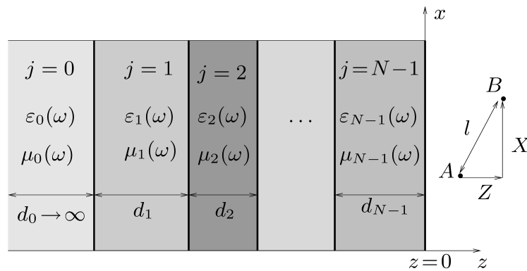
Figure 1: Sketch of the planar multilayer medium.

According to the decomposition (54) of the Green tensor, the two-atom potential $U_{AB}$, Eq. (50), can be decomposed into three parts,

$$U_{AB}(\mathbf{r}_{A},\mathbf{r}_{B}) = U_{AB}^{(0)}(\mathbf{r}_{A},\mathbf{r}_{B})+U_{AB}^{(1)}(\mathbf{r}_{A},\mathbf{r}_{B})$$ (72)

$$+U_{AB}^{(2)}(\mathbf{r}_{A},\mathbf{r}_{B}),$$

where

$$U_{AB}^{(0)}(\mathbf{r}_{A},\mathbf{r}_{B})=-\frac{\hbar\mu_{0}^{2}}{2\pi}\int_{0}^{\infty}{\mathrm{d}}u\,u^{4}\alpha_{A}(iu)\alpha_{B}(iu)\\ \times\,\mathrm{Tr}\bigl{[}{\bm{G}}^{(0)}(\mathbf{r}_{A},\mathbf{r}_{B},iu)\!\cdot\!{\bm{G}}^{(0)}(\mathbf{r}_{B},\mathbf{r}_{A},iu)\bigr{]}$$ (73)

is the bulk-part contribution, which is given by Eq. (IV.1) with $n(iu)$ $\!\equiv$ $\!1$ $\!\equiv$ $\!\mu(iu)$,

$$U_{AB}^{(1)}(\mathbf{r}_{A},\mathbf{r}_{B})=-\frac{\hbar\mu_{0}^{2}}{\pi}\int_{0}^{\infty}{\mathrm{d}}u\,u^{4}\alpha_{A}(iu)\alpha_{B}(iu)\\ \times\,\mathrm{Tr}\big{[}{\bm{G}}^{(0)}(\mathbf{r}_{A},\mathbf{r}_{B},iu)\!\cdot\!{\bm{G}}^{(1)}(\mathbf{r}_{B},\mathbf{r}_{A},iu)\big{]}\\ =-\frac{\hbar\mu_{0}^{2}}{32\pi^{3}l}\int_{0}^{\infty}{\mathrm{d}}u\,u^{4}\alpha_{A}(iu)\alpha_{\mathrm{B}}(iu)\,e^{-lu/c}\int_{0}^{\infty}{\rm d}q\,q\\ \times\,e^{-b_{N}Z_{+}}\left(\bigg{\{}\bigg{[}2f(\xi)-g(\xi)\frac{X^{2}}{l^{2}}\bigg{]}\bigg{[}\frac{r_{N}^{s}}{b_{N}}-\frac{b_{N}}{k_{N}^{2}}\,r_{N}^{p}\bigg{]}\right.\\ -2\bigg{[}f(\xi)-g(\xi)\frac{Z^{2}}{l^{2}}\bigg{]}\frac{q^{2}}{b_{N}k_{N}^{2}}\,r_{N}^{p}\bigg{\}}J_{0}(qX)\\ \left.-g(\xi)\frac{X^{2}}{l^{2}}\bigg{[}\frac{r_{N}^{s}}{b_{N}}+\frac{b_{N}}{k_{N}^{2}}\,r_{N}^{p}\bigg{]}J_{2}(qX)\right)$$ (74)

comes from the cross term of bulk and scattering parts [with $f(x)$ and $g(x)$ being defined by Eqs. (57) and (58), respectively, $\xi$ $\!=$ $\!c/(lu)$, and $Z$ $\!=$ $\!z_{B}$ $\!-$ $\!z_{A}$], and

$$U_{AB}^{(2)}(\mathbf{r}_{A},\mathbf{r}_{B})=-\frac{\hbar\mu_{0}^{2}}{2\pi}\int_{0}^{\infty}\!{\mathrm{d}}u\,u^{4}\alpha_{A}(iu)\alpha_{B}(iu)\\ \times\,\mathrm{Tr}\big{[}{\bm{G}}^{(1)}(\mathbf{r}_{A},\mathbf{r}_{B},iu)\!\cdot\!{\bm{G}}^{(1)}(\mathbf{r}_{B},\mathbf{r}_{A},iu)\big{]}\\ =-\frac{\hbar\mu_{0}^{2}}{64\pi^{3}}\int_{0}^{\infty}{\mathrm{d}}u\,u^{4}\alpha_{A}(iu)\alpha_{\mathrm{B}}(iu)\int_{0}^{\infty}\!{\rm d}q\,q\int_{0}^{\infty}\!{\rm d}q^{\prime}\,q^{\prime}\\ \times e^{-(b_{N}+b_{N}^{\prime})Z_{+}}\biggl{\{}\bigg{[}\frac{r_{N}^{s}r_{N}^{s\prime}}{b_{N}b_{N}^{\prime}}+\frac{r_{N}^{p}r_{N}^{p\prime}}{k_{N}^{4}}\bigg{(}b_{N}b_{N}^{\prime}+\frac{2q^{2}q^{\prime 2}}{b_{N}b_{N}^{\prime}}\bigg{)}\\ -\frac{b_{N}^{\prime}r_{N}^{s}r_{N}^{p\prime}}{b_{N}{k_{N}}^{2}}-\frac{b_{N}r_{N}^{s\prime}r_{N}^{p}}{b_{N}^{\prime}{k_{N}}^{2}}\bigg{]}J_{0}(qX)J_{0}(q^{\prime}X)\\ +\frac{4qq^{\prime}r_{N}^{p}r_{N}^{p\prime}}{k_{N}^{4}}J_{1}(qX)J_{1}(q^{\prime}X)+\bigg{[}\frac{r_{N}^{s}r_{N}^{s\prime}}{b_{N}b_{N}^{\prime}}\\ +\frac{b_{N}b_{N}^{\prime}r_{N}^{p}r_{N}^{p\prime}}{k_{N}^{4}}+\frac{b_{N}^{\prime}r_{N}^{s}r_{N}^{p\prime}}{b_{N}{k_{N}}^{2}}+\frac{b_{N}r_{N}^{s\prime}r_{N}^{p}}{b_{N}^{\prime}{k_{N}}^{2}}\bigg{]}\\ \times J_{2}(qX)J_{2}(q^{\prime}X)\biggr{\}}$$ (75)

is the scattering-part contribution [$b_{N}^{\prime}$ $\!=$ $\!b_{N}(q^{\prime},u)$, $r^{\sigma\prime}_{N}$ $\!=r^{\sigma}_{N}(q^{\prime},u)$].

IV.2.1 Perfectly reflecting plate

Let us consider the case $N$ $\!=$ $\!1$ (Fig. 2) in more detail and begin with the limiting case of a perfectly reflecting plate,

$$r_{p}\equiv r^{p}_{1}=\pm 1,\qquad r_{s}\equiv r^{s}_{1}=\mp 1,$$ (76)

where the upper (lower) sign corresponds to a perfectly conducting (permeable) plate. In the retarded limit, where $l,z_{\mathrm{A}},z_{\mathrm{B}}$ $\!\gg$ $\!c/\omega_{\mathrm{min}}$ [$\omega_{\mathrm{min}}$ $\!=$ $\mathrm{min}(\{\omega_{A^{\prime}}^{n}|A^{\prime}\!=\!A,B;\,n\!=\!1,2,\ldots\})$], $U_{AB}^{(0)}$ is given by Eq. (62) with $n(0)$ $\!\equiv$ $\!1$ $\!\equiv$ $\!\mu(0)$, whereas $U_{AB}^{(1)}$ [Eq. (74)] and $U_{AB}^{(2)}$ [Eq. (75)] can be given in closed form only in some special cases. If $X$ $\!\ll$ $\!Z_{+}$ (cf. Fig. 2), we derive, on using the relevant elements of the scattering Green tensor as given in App. C [Eqs. (C) and (C)],

$$U_{AB}^{(1)}=\pm\frac{32}{23}\,\frac{X^{2}+6l^{2}}{l^{3}Z_{+}(l+Z_{+})^{5}}\,C_{\mathrm{r}}\,,$$ (77)

$$U_{AB}^{(2)}=-\frac{C_{\mathrm{r}}}{Z_{+}^{7}}\,,$$ (78)

where $C_{\mathrm{r}}$ is given by Eq. (63) with $\varepsilon(0)$ $\!\equiv$ $\!1$ $\!\equiv$ $n(0)$. Thus, recalling Eq. (62), the interaction potential (72) reads

$$U_{AB}=\Big{[}-\frac{1}{l^{7}}\pm\frac{32}{23}\frac{X^{2}+6l^{2}}{l^{3}Z_{+}(l+Z_{+})^{5}}-\frac{1}{Z_{+}^{7}}\Big{]}C_{\mathrm{r}}\,.$$ (79)

In particular, if $z_{A}$ $\!\ll$ $\!z_{B}$, or equivalently $Z_{+}$ $\!\simeq$ $\!Z\simeq l$, from Eqs. (77) and (78) it follows that

$$U_{AB}^{(1)}=\mp\frac{6}{23}\,U_{AB}^{(0)}\,,$$ (80)

$$U_{AB}^{(2)}=U_{AB}^{(0)}\,,$$ (81)

so the interaction potential $U_{AB}$, Eq. (72), is enhanced by the presence of the perfectly reflecting plate:

$$U_{AB}=\left\{\begin{array}[]{cc}\frac{40}{23}U_{AB}^{(0)}&\ \mathrm{for}\ r_{p(s)}=\raisebox{2.5pt}{$+$}\raisebox{-2.5pt}{{\scriptsize(}$\!-\!$\scriptsize{)}}1,\\ &\\ \frac{52}{23}U_{AB}^{(0)}&\ \mathrm{for}\ r_{p(s)}=\raisebox{2.5pt}{$-$}\raisebox{-2.5pt}{{\scriptsize(}$\!+\!$\scriptsize{)}}1.\\ \end{array}\right.$$ (82)

Figure 2: Two atoms near a perfectly reflecting plate.

Next, we discuss the behavior of $U_{AB}$ in the case where the condition $z_{A}$ $\!\ll$ $\!z_{B}$ is not valid. Since the bulk part $U_{AB}^{(0)}$ [first term in the square brackets in Eq. (79)] is negative, the interaction potential is enhanced (reduced) by the plate if the scattering part $U_{AB}^{(1)}$ $\!+$ $\!U_{AB}^{(2)}$ [second and third terms in the square brackets in Eq. (79)] is negative (positive). In the case of a perfectly conducting plate, it is seen that especially for $Z$ $\!=$ $\!0$, briefly referred to as the parallel case, $U_{AB}^{(1)}$ $\!+$ $\!U_{AB}^{(2)}$ is positive, and hence the interaction potential is reduced by the plate, whereas for $X$ $\!=$ $\!0$, briefly referred to as the vertical case, $U_{AB}^{(1)}$ $\!+$ $\!U_{AB}^{(2)}$ is positive and the interaction potential is reduced iff

$$z_{B}/z_{A}\lesssim 4.90,$$ (83)

where, without loss of generality, atom $A$ is assumed to be closer to the plate than atom $B$. It is apparent from Eq. (79) that for a perfectly permeable plate $U_{AB}^{(1)}$ $\!+$ $\!U_{AB}^{(2)}$ is always negative, and hence the interaction potential is always enhanced by the plate.

Let us now turn to the nonretarded limit, where $l,z_{A},z_{B}$ $\!\ll$ $\!c/\omega_{\mathrm{max}}$ [$\omega_{\mathrm{max}}$ $\!=$ $\!\mathrm{max}(\{\omega_{A^{\prime}}^{n}|A^{\prime}\!=\!A,B;\,n$ $\!=1,2,\ldots\})$], and $U_{AB}^{(0)}$ is given by Eq. (64) [$\varepsilon(iu)$ $\!\equiv$ $\!1$]. From Eqs. (74) and (75) we derive, on making use of the relevant elements of the scattering Green tensor as given in App. C [Eqs. (137)–(140)],

$$U_{AB}^{(1)}=\pm\frac{4X^{4}-2Z^{2}Z_{+}^{2}+X^{2}(Z_{+}^{2}+Z^{2})}{3l^{5}l_{+}^{5}}\,C_{\mathrm{nr}}\,,$$ (84)

$$U_{AB}^{(2)}=-\frac{C_{\mathrm{nr}}}{l_{+}^{6}}$$ (85)

($l_{+}$ $\!=$ $\!\sqrt{X^{2}+Z_{+}^{2}}$), where $C_{\mathrm{nr}}$ is given by Eq. (65) with $\varepsilon(iu)$ $\!\equiv$ $\!1$. Hence, the interaction potential (72), reads, on recalling Eq. (64),

$$U_{AB}=\bigg{[}-\frac{1}{l^{6}}\pm\frac{4X^{4}-2Z^{2}Z_{+}^{2}+X^{2}(Z_{+}^{2}+Z^{2})}{3l^{5}l_{+}^{5}}-\frac{1}{l_{+}^{6}}\bigg{]}C_{\mathrm{nr}}\,.$$ (86)

Let us again consider the effect of the plate on the interaction potential for the parallel and vertical cases. In the parallel case, Eq. (86) takes the form

$$U_{AB}=\bigg{[}-\frac{1}{l^{6}}\pm\frac{4l^{2}+Z_{+}^{2}}{3l^{3}(l^{2}+Z_{+}^{2})^{\frac{5}{2}}}-\frac{1}{(l^{2}+Z_{+}^{2})^{3}}\bigg{]}C_{\mathrm{nr}}\,,$$ (87)

which in the on-surface limit $Z_{+}$ $\!\to$ $\!0$ approaches

$$U_{AB}=\left\{\begin{array}[]{cc}\frac{2}{3}U_{AB}^{(0)}&\ {\mathrm{for}}\ r_{p(s)}=\raisebox{2.5pt}{$+$}\raisebox{-2.5pt}{{\scriptsize(}$\!-\!$\scriptsize{)}}1,\\ \\ \frac{10}{3}U_{AB}^{(0)}&\ {\mathrm{for}}\ r_{p(s)}=\raisebox{2.5pt}{$-$}\raisebox{-2.5pt}{{\scriptsize(}$\!+\!$\scriptsize{)}}1.\\ \end{array}\right.$$ (88)

It can be seen easily that the term $U_{AB}^{(1)}$ [second term in the square brackets in Eq. (87)] dominates the term $U_{AB}^{(2)}$ [third term in the square brackets in Eq. (87)], so $U_{AB}^{(1)}$ $\!+$ $\!U_{AB}^{(2)}$ is positive (negative) for a perfectly conducting (permeable) plate, and hence the interaction potential is reduced (enhanced) due to the presence of the plate.

In the vertical case, from Eq. (86) the interaction potential is obtained to be

$$U_{AB}=\bigg{[}-\frac{1}{l^{6}}\mp\frac{2}{3Z_{+}^{3}l^{3}}-\frac{1}{Z_{+}^{6}}\bigg{]}C_{\mathrm{nr}}\,.$$ (89)

It is obvious that $U_{AB}^{(1)}$ $\!+$ $\!U_{AB}^{(2)}$ [second and third terms in Eq. (89)] is negative when the plate is perfectly conducting, thereby enhancing the interaction potential since $U_{AB}^{(0)}$ [first term in Eq. (89)] is negative. In the case of a perfectly permeable plate, $U_{AB}^{(1)}+U_{AB}^{(2)}$ is positive iff

$$\frac{z_{B}}{z_{A}}<1+\frac{2}{(\frac{3}{2})^{\frac{1}{3}}-1}\simeq 14.82,$$ (90)

where atom $A$ is again assumed to be closer to the plate than atom $B$.

Since $U_{AB}^{(0)}$ and $U_{AB}^{(2)}$ are negative in all cases, the realization of enhancement or reduction of the interaction potential depends only on the sign of $U_{AB}^{(1)}$ and its magnitude compared to that of $U_{AB}^{(2)}$.

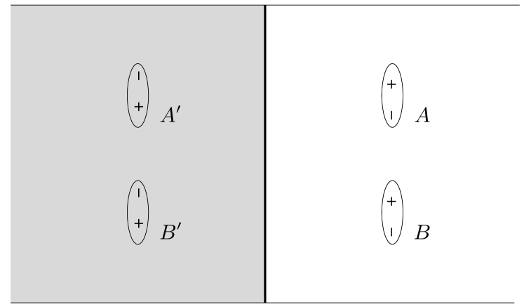
Figure 3: Two electric dipoles near a perfectly conducting plate (parallel case).

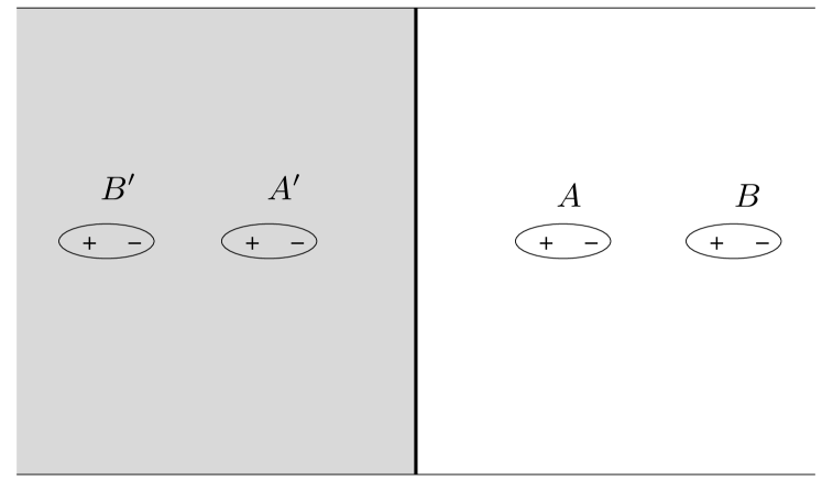
Figure 4: Two electric dipoles near a perfectly conducting plate (vertical case).

In particular, the results for the non-retarded limit (the sign of $U_{AB}^{(1)}$ being summarized in Tab. 1) can be explained by using the method of image charges, where the two-atom vdW interaction is regarded as being due to the interactions between fluctuating dipoles $A$ and $B$ and their images ${A}^{\prime}$ and ${B}^{\prime}$ in the plate, with

$$\hat{H}_{\mathrm{int}}=\hat{V}_{AB}+\hat{V}_{AB^{\prime}}+\hat{V}_{BA^{\prime}}$$ (91)

being the corresponding interaction Hamiltonian. Here, $\hat{V}_{AB}$ denotes the direct interaction between dipole $A$ and dipole $B$, while $\hat{V}_{AB^{\prime}}$ and $\hat{V}_{BA^{\prime}}$ denote the indirect interaction between each dipole and the image induced by the other one in the plate. The leading contribution to the energy shift is of second order in $H_{\mathrm{int}}$,

$$\Delta E_{AB}=-\sideset{}{{}^{\prime}}{\sum}_{n,m}\frac{\langle 0_{A},0_{B}|\hat{H}_{\mathrm{int}}|n_{A},m_{B}\rangle}{\hbar(\omega_{A}^{n}+\omega_{B}^{m})}\\ \times\,\langle n_{A},m_{B}|\hat{H}_{\mathrm{int}}|0_{A},0_{B}\rangle.$$ (92)

In this approach, $U_{AB}^{(0)}$ corresponds to the product of two direct interactions, so it is negative in agreement with Eq. (86), because of the minus sign on the r.h.s. of Eq. (92). Accordingly, $U_{AB}^{(2)}$ is due to the product of two indirect interactions and is also negative—in agreement with Eq. (86). The terms containing one direct and one indirect interaction are contained in $U^{(1)}_{AB}$ and determine its sign. We can hence predict the sign of $U^{(1)}_{AB}$ from a graphical construction of the image charges, as sketched in Figs. 3–6.

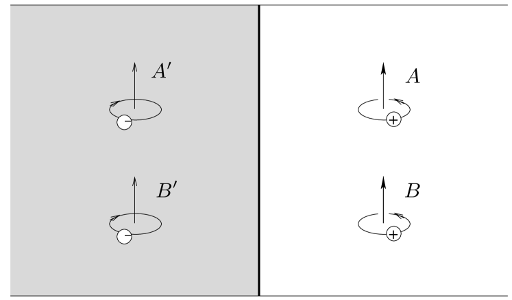
Figure 5: Two magnetic dipoles near a perfectly conducting plate (parallel case).

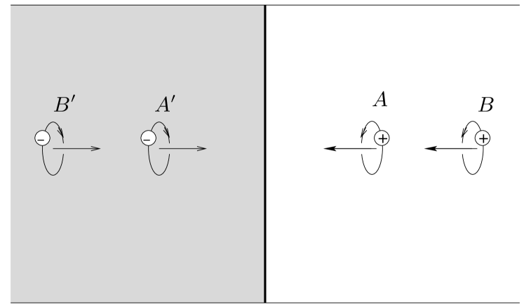
Figure 6: Two magnetic dipoles near a perfectly conducting plate (vertical case).

Figure 3 shows two electric dipoles in front of a perfectly conducting plate in the parallel case. The configuration of dipoles and images indicates repulsion between dipole $A(B)$ and dipole $B^{\prime}(A^{\prime})$, so $U_{AB}^{(1)}$ is positive, in agreement with Tab. 1. On the contrary, in the vertical case from Fig. 4 attraction is indicated, i.e., negative $U_{AB}^{(1)}$, which is also in agreement with Tab. 1.

	conducting plate	permeable plate
parallel case	$+$	$-$
vertical case	$-$	$+$

Table 1: Sign of $U_{AB}^{(1)}$ for a perfectly reflecting plate.

The case of two electric dipoles in front of a perfectly permeable plate can be treated by considering two magnetic dipoles in front of a perfectly conducting plate, as the two situations are equivalent due to the duality between electric and magnetic fields in the absence of free charges or currents. From Figs. 5 (parallel case) and 6 (vertical case) it is apparent that the interaction between dipole $A(B)$ and dipole $B^{\prime}(A^{\prime})$ is attractive in the parallel case and repulsive in the vertical case, again confirming the sign of $U_{AB}^{(1)}$ as given in Tab. 1. When the dipole–dipole separation in Fig. 6 is sufficiently small compared with the dipole–surface separations, then the direct interaction between the two dipoles is expected to be stronger than their indirect interaction via the image dipoles. As a result, $U_{AB}^{(1)}$ will be the dominant term in $U_{AB}^{(1)}$ $\!+$ $\!U_{AB}^{(2)}$ and $U_{AB}^{(1)}$ $\!+$ $\!U_{AB}^{(2)}$ becomes positive. However, when the dipole–dipole separation exceeds the dipole–surface separations, then the indirect interaction may become comparable to the direct one, and $U_{AB}^{(2)}$ may be the dominant term, leading to negative $U_{AB}^{(1)}+U_{AB}^{(2)}$. The image dipole model hence gives also a qualitative explanation of the condition (90).

IV.2.2 Semi-infinite magnetodielectric half space

Let us now abandon the assumption of perfect reflectivity and consider a magnetodielectric plate of permittivity $\varepsilon(\omega)$ and permeability $\mu(\omega)$. To be more specific, we restrict our attention to a sufficiently thick plate so that the model of a semi-infinite half space applies. In this case, Eq. (IV.2) for the reflection coefficients reduces to

$$r_{\sigma}\equiv r_{1}^{\sigma}=\frac{\lambda_{0}^{\sigma}b-b_{0}}{\lambda_{0}^{\sigma}b+b_{0}}\,,$$ (93)

with $b$ $\!\equiv$ $\!b_{1}$ $\!=$ $\!\sqrt{u^{2}/c^{2}\!+\!q^{2}}$, $b_{0}$ $\!=$ $\!\sqrt{\varepsilon(iu)\mu(iu)u^{2}/c^{2}\!+\!q^{2}}$, $\lambda_{0}^{s}$ $\!=$ $\!\mu(iu)$, and $\lambda_{0}^{p}$ $\!=$ $\!\varepsilon(iu)$.

In the retarded limit, $l,z_{A},z_{B}$ $\!\gg$ $\!c/\omega_{\mathrm{min}}$ [with $\omega_{\mathrm{min}}$ being defined as above Eq. (61)] we may again replace the atomic polarizability and the permittivity and permeability of the plate by their static values. Replacing the integration variable $q$ in Eq. (74) by $v$ $\!=$ $\!b_{1}c/u$ [cf. Eq. (132)] leads to

$$U_{AB}^{(1)}(\mathbf{r}_{A},\mathbf{r}_{B})=\frac{\hbar c}{32\pi^{3}l^{3}\varepsilon_{0}^{2}}\alpha_{A}(0)\alpha_{B}(0)\int_{1}^{\infty}{\rm d}v\,$$

$$\quad\times\bigg{\{}\bigg{[}v^{2}\bigg{(}Z^{2}A_{5-}+(Z^{2}-2X^{2})\bigg{[}\frac{A_{4-}}{l}+\frac{A_{3-}}{l^{2}}\bigg{]}$$

$$\qquad+l^{2}A_{5+}+lA_{4+}+A_{3+}\bigg{)}+2(v^{2}-1)\bigg{(}X^{2}B_{5}$$

$$\qquad+\big{(}X^{2}-2Z^{2}\big{)}\bigg{[}\frac{B_{4}}{l}+\frac{B_{3}}{l^{2}}\bigg{]}\bigg{)}\bigg{]}r_{p}$$

$$\qquad+\bigg{(}Z^{2}A_{5+}+\big{(}Z^{2}-2X^{2}\big{)}\bigg{[}\frac{A_{4+}}{l}+\frac{A_{3+}}{l^{2}}\bigg{]}$$

$$\qquad+l^{2}A_{5-}+lA_{4-}+A_{3-}\bigg{)}r_{s}\bigg{\}},$$ (94)

where, according to Eq. (93), the static reflection coefficients are given by

$$r_{s}=r_{s}(v)=\frac{\mu(0)v-\sqrt{\varepsilon(0)\mu(0)-1+v^{2}}}{\mu(0)v+\sqrt{\varepsilon(0)\mu(0)-1+v^{2}}}\,,$$ (95)

$$r_{p}=r_{p}(v)=\frac{\varepsilon(0)v-\sqrt{\varepsilon(0)\mu(0)-1+v^{2}}}{\varepsilon(0)v+\sqrt{\varepsilon(0)\mu(0)-1+v^{2}}}\,,$$ (96)

and

$$A_{n\pm}=\frac{1}{c^{n+1}}\int_{0}^{\infty}\mathrm{d}u\,u^{n}\,e^{-au/c}\big{[}J_{0}(\beta u/c)\pm J_{2}(\beta u/c)\big{]},$$ (97)

$$B_{n}=\frac{1}{c^{n+1}}\int_{0}^{\infty}{\mathrm{d}}u\,u^{n}e^{-au/c}J_{0}(\beta u/c),$$ (98)

with $\beta$ $\!=$ $\!X\sqrt{v^{2}-1}$ and $a$ $\!=$ $\!l$ $\!+$ $\!vZ_{+}$ (for explicit expressions of $A_{n\pm}$ and $B_{n}$, see App. D). Similarly, Eq. (75) reduces to

$$U_{AB}^{(2)}=-\frac{\hbar\mu_{0}^{2}}{64\pi^{3}c^{2}}\,\alpha_{A}(0)\alpha_{B}(0)\int_{1}^{\infty}{\rm d}v\int_{1}^{\infty}{\rm d}v^{\prime}$$

$$\quad\times\biggl{\{}\Big{(}r_{p}r_{p}^{\prime}\big{[}3v^{2}v^{\prime 2}-2(v^{2}+v^{\prime 2})+2\big{]}+r_{s}r_{s}^{\prime}-r_{s}r_{p}^{\prime}v^{\prime 2}$$

$$\quad-r_{p}r_{s}^{\prime}v^{2}\Big{)}M_{0}+4vv^{\prime}\sqrt{v^{2}-1}\sqrt{v^{\prime 2}-1}r_{p}r_{p}^{\prime}M_{1}$$

$$\quad+\big{(}r_{s}r_{s}^{\prime}+r_{p}r_{p}^{\prime}v^{2}v^{\prime 2}+r_{s}r_{p}^{\prime}v^{\prime 2}+r_{p}r_{s}^{\prime}v^{2}\big{)}M_{2}\biggr{\}}$$ (99)

[$r^{\prime}_{\sigma}=r_{\sigma}(v^{\prime})$], where

$$M_{n}=\int_{0}^{\infty}{\mathrm{d}}u\,u^{6}e^{-(v+v^{\prime})Z_{+}u/c}J_{n}(\beta u/c)J_{n}(\beta^{\prime}u/c)$$ (100)

($\beta^{\prime}$ $\!=$ $\!X\sqrt{v^{\prime 2}-1}$), which can be evaluated analytically only in some special cases. In particular, when $X$ $\!\ll$ $\!Z_{+}$, then approximately

$$M_{n}=J_{n}^{2}(0)\int_{0}^{\infty}{\mathrm{d}}u\,u^{6}e^{-(v+v^{\prime})Z_{+}u/c}=\frac{720c^{7}}{(v+v^{\prime})^{7}Z_{+}^{7}}\,\delta_{n0}.$$ (101)

In the nonretarded limit, $l,z_{A},z_{B}$ $\!\ll$ $\!c/[n(0)\omega_{\mathrm{max}}]$ [with $\omega_{\mathrm{max}}$ being defined as above Eq. (64)], $U_{AB}^{(1)}$ and $U_{AB}^{(2)}$ can be obtained by using in Eqs. (74) and (75), respectively, the relevant elements of the scattering part of Green tensor as given in App. C. In the case of a purely dielectric half space ($\mu$ $\!\equiv$ $\!1$) we derive [Eqs. (143)–(146)]

$$U_{AB}=-\frac{C_{\mathrm{nr}}}{l^{6}}\\ +\frac{\big{[}4X^{4}-2Z^{2}Z_{+}^{2}+X^{2}(Z^{2}+Z_{+}^{2})\big{]}C^{(1)}_{\mathrm{nr}}}{l^{5}l_{+}^{5}}-\frac{C^{(2)}_{\mathrm{nr}}}{l_{+}^{6}}\,,$$ (102)

where $C_{\mathrm{nr}}$ is given by Eq. (65) with $\varepsilon(iu)$ $\!\equiv$ $\!1$, and

$$C^{(1)}_{\mathrm{nr}}=\frac{\hbar}{16\pi^{3}\varepsilon_{0}^{2}}\int_{0}^{\infty}{\mathrm{d}}u\,\alpha_{A}(iu)\alpha_{\mathrm{B}}(iu)\frac{\varepsilon(iu)-1}{\varepsilon(iu)+1}\,,$$ (103)

$$C^{(2)}_{\mathrm{nr}}=\frac{3\hbar}{16\pi^{3}\varepsilon_{0}^{2}}\int_{0}^{\infty}{\rm d}u\,\alpha_{A}(iu)\alpha_{B}(iu)\bigg{[}\frac{\varepsilon(iu)-1}{\varepsilon(iu)+1}\bigg{]}^{2}\!.$$ (104)

In particular in the limiting case when $l$ $\!\ll$ $\!Z_{+}$, Eq. (102) reduces to

$$U_{AB}=-\frac{C_{\mathrm{nr}}}{l^{6}}+\frac{\big{(}X^{2}-2Z^{2}\big{)}C^{(1)}_{\mathrm{nr}}}{l^{5}Z_{+}^{3}}\,.$$ (105)

It is seen that the second term on the r.h.s. of this equation is positive (negative) in the parallel (vertical) case, so the vdW potential is reduced (enhanced) by the presence of the dielectric half space. In the case of a purely magnetic half space ($\varepsilon$ $\!\equiv$ $\!1$) we derive [Eqs. (C)–(150)]

$$U_{AB}=-\frac{C_{\mathrm{nr}}}{l^{6}}+\frac{\big{[}Z^{2}-2X^{2}+3Z_{+}(l_{+}-Z_{+})\big{]}C_{\mathrm{nr}}^{(3)}}{l^{5}l_{+}}\,,$$ (106)

where

$$C_{\mathrm{nr}}^{(3)}=\frac{\hbar}{64\pi^{3}\varepsilon_{0}^{2}c^{2}}\int_{0}^{\infty}{\rm d}u\,u^{2}\alpha_{A}(iu)\alpha_{B}(iu)\\ \times\;\frac{[\mu(iu)-1][\mu(iu)-3]}{\mu(iu)+1}\,.$$ (107)

Note that $U_{AB}^{(2)}$ does not contribute to the asymptotic nonretarded two-atom vdW potential $U_{AB}$ for the purely magnetic half space. In particular in the limiting case when $X$ $\!\ll$ $\!Z_{+}$, Eq. (106) reduces to

$$U_{AB}=-\frac{C_{\mathrm{nr}}}{l^{6}}+\frac{\big{(}2Z^{2}-X^{2}\big{)}C_{\mathrm{nr}}^{(3)}}{2l^{5}Z_{+}}\,.$$ (108)

It is seen that the second term in the r.h.s. of this equation is negative (positive) in the parallel (vertical) case, so the vdW potential is enhanced (reduced) due to the presence of the magnetic half space.

It should be pointed out that the nonretarded limit for the magnetodielectric half space is in general incompatible with the limit of perfect reflectivity [$\varepsilon(iu)\rightarrow\infty$ or $\mu(iu)$ $\!\to$ $\!\infty$] considered in Sec. IV.2.1, as is clearly seen from the condition given above Eq. (102) [cf. also the expansions (141) and (142), which are not well-behaved in the limit of perfect reflectivity]. As a consequence, Eq. (106) does not reduce to Eq. (86) via the limit $\mu(iu)$ $\!\to$ $\!\infty$. It is therefore remarkable that the result for a purely dielectric half space, Eq. (102), does reduce to Eq. (86) in the limit $\varepsilon(iu)$ $\!\to$ $\!\infty$, as already noted in Ref. Babiker76 in the case of the single-atom potential.

Figure 7: The vdW potential for two identical two-level atoms in the parallel case in presence of (a) a purely dielectric half space with $\omega_{\mathrm{P}e}/\omega_{10}$ $\!=$ $\!3$, $\omega_{\mathrm{T}e}/\omega_{10}$ $\!=$ $\!1$, and $\gamma_{e}/\omega_{10}$ $\!=$ $\!0.001$ (b) a purely magnetic half space with $\omega_{\mathrm{P}m}/\omega_{10}$ $\!=$ $\!3$, $\omega_{\mathrm{T}m}/\omega_{10}$ $\!=$ $\!1$, and $\gamma_{m}/\omega_{10}=0.001$ is shown as a function of the atom–atom separation $l$ [$\omega_{10}$ is the atomic transition frequency, and $U_{AB}^{(0)}(l)$ is the potential in free space]. The atom–half-space separations are $z_{A}\!=\!z_{B}$ $\!=$ $\!0.01c/\omega_{10}$ (solid line), $0.2c/\omega_{10}$ (dashed line), and $c/\omega_{10}$ (dotted line).

Figures 7–9 show the results of exact (numerical) calculation of the vdW interaction between two identical two-level atoms near a semi-infinite half space, as given by Eq. (72) together with Eqs. (IV.1), (74), and (75). In the figures the potentials and the forces are normalized w.r.t. their values in free space as given by Eq. (IV.1) [$n(iu)$ $\equiv$ $\!1$ $\!\equiv$ $\!\mu(iu)$]. In the calculations, we have used single-resonance Drude–Lorenz-type electric and magnetic susceptibilities of the half space,

$$\varepsilon(\omega)=1+\frac{\omega_{\mathrm{P}e}^{2}}{\omega^{2}_{{\mathrm{T}e}}-\omega^{2}-i\omega\gamma_{e}}\,,$$ (109)

$$\mu(\omega)=1+\frac{\omega_{\mathrm{P}m}^{2}}{\omega^{2}_{\mathrm{T}m}-\omega^{2}-i\omega\gamma_{m}}\,.$$ (110)

Figure 8: The vdW potential for two two-level atoms in the vertical case in the presence of (a) a purely dielectric half space and (b) a purely magnetic half space is shown as a function of the atom–atom separation $l$. The distance between atom $A$ (which is closer to the surface of the half space than atom $B$) and the surface is equal to $0.01c/\omega_{10}$ (solid line), $0.2c/\omega_{10}$ (dashed line), and $c/\omega_{10}$ (dotted line). All other parameters are the same as in Fig. 7.

Figure 9: The vdW force acting on atom $A$ (which is closer to the surface of the half space than atom $B$) in the presence of (a) a purely dielectric half space and (b) a purely magnetic half space is shown as a function of the atom–atom separation $l$. All parameters are the same as in Fig. 8.

From the figures it is seen that the vdW interaction is unaffected by the presence of the half space for atom–half-space separations that are much greater than the interatomic separations, while an asymptotic enhancement or reduction of the interaction is observed in the opposite limit.

Figure 7(a) shows the dependence of the normalized interaction potential $U_{AB}(l)$ on the atom–atom separation $l$ in the parallel case ($Z$ $\!=$ $\!0$) for different values of the distance $z_{A}$ $\!(=$ $\!z_{B})$ of the atoms from a purely dielectric half space. The ratio of the interatomic force along the connecting line of the two atoms, $F_{ABx}(l)$ [Eq. (55)] to the corresponding force in free space, $F^{(0)}_{ABx}(l)$, follows closely the ratio $U_{AB}(l)/U^{(0)}_{AB}(l)$, so that, within the resolution of the figures, the curves for $F_{ABx}(l)/F^{(0)}_{ABx}(l)$ (not shown) would coincide with those for $U_{AB}(l)/U^{(0)}_{AB}(l)$. The figure reveals that due to the presence of the dielectric half space the attractive interaction potential and force are reduced, in agreement with the predictions from the nonretarded limit, Eq. (105). The relative reduction of the potential and the force are not monotonic, there is a value of the atom–atom separation where the reduction is strongest. The $l$-dependence of $U_{AB}(l)/U^{(0)}_{AB}(l)$ in the presence of a purely magnetic half space in the parallel case is shown in Figs. 7(b). Again, the corresponding force ratio $F_{ABx}(l)/F^{(0)}_{ABx}(l)$ (not shown) behaves like $U_{AB}(l)/U^{(0)}_{AB}(l)$. The figure indicates that the presence of a purely magnetic half space enhances the vdW interaction between the two atoms, with the enhancement increasing with the atom-atom separation, in agreement with the nonretarded limit, Eq. (108).

Figure 8 shows $U_{AB}(l)/U^{(0)}_{AB}(l)$ in the vertical case ($X$ $\!=$ $\!0$) when the half space is purely dielectric [Fig. 8(a)] or purely magnetic [Fig. 8(b)]. In the figure, atom $A$ is assumed to be closer to the surface of the half space than atom $B$, and the graphs show the variation of the interaction potential with the atom–atom separation $l$ for different distances $z_{A}$ of atom $A$ from the surface of the half space. It is seen that for a purely dielectric half space the potential is enhanced compared to the one observed in the free-space case—in agreement with Eq. (105). Note that there are values of the atom–atom separation at which the enhancement is strongest. For a purely magnetic half space, the potential is seen to be typically enhanced although for very small atom–atom separations a reduction appears [inset in Fig. 8(b)]—in agreement with Eq. (108). As in the parallel case, the relative enhancement is monotonic. Whereas the force $F_{BAz}(l)/F^{(0)}_{BAz}(l)$ for the force acting on atom $B$ (not shown) again follows closely the potential ratio $U_{AB}(l)/U^{(0)}_{AB}(l)$, the ratio $F_{ABz}(l)/F^{(0)}_{ABz}(l)$, for the force acting on atom $A$ noticeably differs from $U_{AB}(l)/U^{(0)}_{AB}(l)$, as can be seen from comparing Figs. 8 and 9. Clearly, the reason must be seen in the different atom–atom and atom–half-space directions in the two cases (cf. Figs. 4 and 6).

Figs. 7(a) and 8(a) showing the interaction potential of two atoms in the presence of a purely dielectric half space in the parallel and vertical cases, respectively cover the results shown in Ref. Cho on a different scale. The results here are more complete because they show that the relative potential does not have the monotonic behavior suggested by the figures in Ref. Cho .

V Summary and Conclusions

Based on macroscopic QED in linear, causal media, we have obtained a general formula for the vdW potential of two ground-state atoms in the presence of an arbitrary arrangement of dispersing and absorbing magnetodielectric media by calculating the leading-(4th) order shift of the ground-state energy of the overall system. The result has been applied to two atoms (i) in bulk material (without taking into account local-field corrections), (ii) in the presence of a perfectly reflecting plate, and (iii) in the presence of a semi-infinite magnetodielectric half space. It has been found that the presence of a bulk magnetodielectric medium will reduce the interaction potential w.r.t. its well-known free-space value.

We have further shown that in the presence of a perfectly reflecting plate the vdW interaction can be enhanced or reduced depending on the (electric/magnetic) nature of the plate and the (parallel/vertical) alignment of the atoms. In particular, in the nonretarded limit these effects can be qualitatively explained using the method of image dipoles.

Finally, we have calculated the vdW potential in the presence of a magnetodielectric half space. The analytical results show that in the nonretarded limit the potential in the case of a purely dielectric half space is reduced (enhanced) in the parallel (vertical) case compared to its value in free space, while in the case of a purely magnetic half space it is enhanced (reduced) for parallel (vertical) alignment of the two atoms. The results for a purely dielectric half space are in qualitative agreement with those for the perfectly conducting plate, while for a magnetic plate the results for finite permeability disagree with those for the perfectly reflecting case in the asymptotic power laws—owing to the fact that the two limits of perfect reflectivity and nonretarded distance do not commute.

The numerical computation of the interaction potential in the whole distance regime confirms the analytical results. In addition, it shows that the relative enhancement/reduction of the vdW interaction is not always monotonous, but may in general display maxima or minima, in particular in the case of a purely dielectric half space.

Appendix A Intermediate states and interaction matrix elements

The intermediate states contributing to the two-atom vdW interaction according to Eq. (III) are listed in the first three columns of Tab. 2; the corresponding matrix elements of the interaction Hamiltonian (30) [together with Eqs. (8) and (25)] can be found by recalling the commutation relations (4) and (5) and using the relations (13) and (II). For example, for case (1) in Tab. 2 this leads to

Case	$|I\rangle$	$|II\rangle$	$|III\rangle$	Denominator
($1$)	$|n_{A},0_{B}\rangle|1^{(1)}\rangle$	$|0_{A},0_{B}\rangle|1^{(2)},1^{(3)}\rangle$	$|0_{A},m_{B}\rangle|1^{(4)}\rangle$	$D_{\mathrm{i}}=(\omega_{A}^{n}+\omega^{\prime})(\omega^{\prime}+\omega)(\omega_{B}^{m}+\omega^{\prime})$,
				$D_{\mathrm{ii}}=(\omega_{A}^{n}+\omega^{\prime})(\omega^{\prime}+\omega)(\omega_{B}^{m}+\omega)$
($2$)	-”-	$|n_{A},m_{B}\rangle|\{0\}\rangle$	$|0_{A},m_{B}\rangle|1^{(2)}\rangle$	$D_{\mathrm{iii}}=(\omega_{A}^{n}+\omega^{\prime})(\omega_{A}^{n}+\omega_{B}^{m})(\omega_{B}^{m}+\omega)$
($3$)	-”-	-”-	$|n_{A},0_{B}\rangle|1^{(2)}\rangle$	$D_{\mathrm{iv}}=(\omega_{A}^{n}+\omega^{\prime})(\omega_{A}^{n}+\omega_{B}^{m})(\omega_{A}^{n}+\omega)$
($4$)	-”-	$|n_{A},m_{B}\rangle|1^{(2)},1^{(3)}\rangle$	$|0_{A},m_{B}\rangle|1^{(4)}\rangle$	$D_{\mathrm{v}}=(\omega_{A}^{n}+\omega^{\prime})(\omega_{A}^{n}+\omega_{B}^{m}+\omega^{\prime}+\omega)(\omega_{B}^{m}+\omega^{\prime})$
($5$)	-”-	-”-	$|n_{A},0_{B}\rangle|1^{(4)}\rangle$	$D_{\mathrm{vi}}=(\omega_{A}^{n}+\omega^{\prime})(\omega_{A}^{n}+\omega_{B}^{m}+\omega^{\prime}+\omega)(\omega_{A}^{n}+\omega)$
($6$)	$|0_{A},m_{B}\rangle|1^{(1)}\rangle$	$|0_{A},0_{B}\rangle|1^{(2)},1^{(3)}\rangle$	$|n_{A},0_{B}\rangle|1^{(4)}\rangle$	$D_{\mathrm{vii}}=(\omega_{B}^{m}+\omega^{\prime})(\omega^{\prime}+\omega)(\omega_{A}^{n}+\omega^{\prime})$,
				$D_{\mathrm{viii}}=(\omega_{B}^{m}+\omega^{\prime})(\omega^{\prime}+\omega)(\omega_{A}^{n}+\omega)$
($7$)	-”-	$|n_{A},m_{B}\rangle|\{0\}\rangle$	$|n_{A},0_{B}\rangle|1^{(2)}\rangle$	$D_{\mathrm{ix}}=(\omega_{B}^{m}+\omega^{\prime})(\omega_{A}^{n}+\omega_{B}^{m})(\omega_{A}^{n}+\omega)$
($8$)	-”-	-”-	$|0_{A},m_{B}\rangle|1^{(2)}\rangle$	$D_{\mathrm{x}}=(\omega_{B}^{m}+\omega^{\prime})(\omega_{A}^{n}+\omega_{B}^{m})(\omega_{B}^{m}+\omega)$
($9$)	-”-	$|n_{A},m_{B}\rangle|1^{(2)},1^{(3)}\rangle$	$|n_{A},0_{B}\rangle|1^{(4)}\rangle$	$D_{\mathrm{xi}}=(\omega_{B}^{m}+\omega^{\prime})(\omega_{A}^{n}+\omega_{B}^{m}+\omega^{\prime}+\omega)(\omega_{A}^{n}+\omega^{\prime})$
($10$)	-”-	-”-	$|0_{A},m_{B}\rangle|1^{(4)}\rangle$	$D_{\mathrm{xii}}=(\omega_{B}^{m}+\omega^{\prime})(\omega_{A}^{n}+\omega_{B}^{m}+\omega^{\prime}+\omega)(\omega_{B}^{m}+\omega)$

Table 2: Intermediate states contributing to the two-atom vdW potential and corresponding denominators.

$$\langle 1^{(1)}|\langle n_{A}|\langle 0_{B}|H_{A\mathrm{F}}+H_{B\mathrm{F}}|0_{A}\rangle|0_{B}\rangle|\{0\}\rangle$$

$$\quad=-\big{[}\mathbf{d}^{n0}_{A}\!\cdot\!\bm{G}^{\ast}_{\lambda_{1}}(\mathbf{r}_{A},\mathbf{r}_{1},\omega_{1})\big{]}_{i_{1}},$$ (111)

$$\langle 1^{(2)},1^{(3)}|\langle 0_{A}|\langle 0_{B}|H_{A\mathrm{F}}+H_{B\mathrm{F}}|n_{A}\rangle|0_{B}\rangle|1^{(1)}\rangle$$

$$\quad=-\frac{1}{\sqrt{2}}\Big{\{}\big{[}\mathbf{d}_{A}^{0n}\!\cdot\!\bm{G}^{\ast}_{\lambda_{3}}(\mathbf{r}_{A},\mathbf{r}_{3},\omega_{3})\big{]}_{i_{3}}\delta^{(12)}$$

$$\qquad\,+\big{[}\mathbf{d}_{A}^{0n}\!\cdot\!\bm{G}^{\ast}_{\lambda_{2}}(\mathbf{r}_{A},\mathbf{r}_{2},\omega_{2})\big{]}_{i_{2}}\delta^{(13)}\Big{\}},$$ (112)

$$\langle 1^{(4)}|\langle 0_{A}|\langle m_{B}|H_{A\mathrm{F}}+H_{B\mathrm{F}}|0_{A}\rangle|0_{B}\rangle|1^{(2)},1^{(3)}\rangle$$

$$\quad=-\frac{1}{\sqrt{2}}\Big{\{}\big{[}\mathbf{d}_{B}^{m0}\!\cdot\!\bm{G}_{\lambda_{3}}(\mathbf{r}_{B},\mathbf{r}_{3},\omega_{3})\big{]}_{i_{3}}\delta^{(24)}$$

$$\qquad\,+\big{[}\mathbf{d}_{B}^{m0}\!\cdot\!\bm{G}_{\lambda_{2}}(\mathbf{r}_{B},\mathbf{r}_{2},\omega_{2})\big{]}_{i_{2}}\delta^{(34)}\Big{\}},$$ (113)

$$\langle\{0\}|\langle 0_{A}|\langle 0_{B}|H_{A\mathrm{F}}+H_{B\mathrm{F}}|0_{A}\rangle|m_{B}\rangle|1^{(4)}\rangle$$

$$\quad=-\big{[}\mathbf{d}_{B}^{0m}\!\cdot\!\bm{G}_{\lambda_{4}}(\mathbf{r}_{B},\mathbf{r}_{4},\omega_{4})\big{]}_{i_{4}},$$ (114)

where $\delta^{(\alpha\beta)}$ is given by Eq. (37). Substituting them into Eq. (III), one obtains Eq. (III) and subsequently Eq. (III), with energy denominators $D_{\mathrm{i}}$ and $D_{\mathrm{ii}}$ as given in Tab. 2. The other denominators listed in the last column of the table follow in a similar way from the respective intermediate states given in the first three columns.

Appendix B Derivation of Eq. (40)

From the energy denominators given in Tab. 2, it is straightforward to obtain

$$\frac{1}{D_{\mathrm{ii}}}+\frac{1}{D_{\mathrm{iii}}}+\frac{1}{D_{\mathrm{viii}}}+\frac{1}{D_{\mathrm{ix}}}+\frac{1}{D_{\mathrm{iv}}}+\frac{1}{D_{\mathrm{x}}}\\ =\frac{1}{\omega_{A}^{n}\!+\!\omega_{B}^{m}}\Biggl{[}\biggl{(}\frac{1}{\omega_{A}^{n}\!+\!\omega}+\frac{1}{\omega_{B}^{m}\!+\!\omega}\biggr{)}\biggl{(}\frac{1}{\omega\!+\!\omega^{\prime}}-\frac{1}{\omega\!-\!\omega^{\prime}}\biggr{)}\\ \quad+\biggl{(}\frac{1}{\omega_{A}^{n}\!+\!\omega^{\prime}}+\frac{1}{\omega_{B}^{m}\!+\!\omega^{\prime}}\biggr{)}\biggl{(}\frac{1}{\omega\!+\!\omega^{\prime}}+\frac{1}{\omega\!-\!\omega^{\prime}}\biggr{)}\Biggr{]}.$$ (115)

Since the denominators appear in combinations of the form of Eq. (III), where they are multiplied with terms (the two factors in square brackets) which are always the same and symmetric with respect to $\omega$ and $\omega^{\prime}$, we may interchange $\omega\leftrightarrow\omega^{\prime}$ in the second term and recombine it with the first one to obtain

$$\frac{1}{D_{\mathrm{ii}}}+\frac{1}{D_{\mathrm{iii}}}+\frac{1}{D_{\mathrm{viii}}}+\frac{1}{D_{\mathrm{ix}}}+\frac{1}{D_{\mathrm{iv}}}+\frac{1}{D_{\mathrm{x}}}\\ \to\frac{2}{\omega_{A}^{n}\!+\!\omega_{B}^{m}}\biggl{(}\frac{1}{\omega_{A}^{n}\!+\!\omega}+\frac{1}{\omega_{B}^{m}\!+\!\omega}\biggr{)}\biggl{(}\frac{1}{\omega\!+\!\omega^{\prime}}-\frac{1}{\omega\!-\!\omega^{\prime}}\biggr{)},$$ (116)

where the symbol $\to$ denotes equality under the double frequency integral. Similarly we have

$$\frac{1}{D_{\mathrm{i}}}+\frac{1}{D_{\mathrm{v}}}+\frac{1}{D_{\mathrm{vi}}}\\ =\frac{1}{(\omega_{A}^{n}\!+\!\omega^{\prime})(\omega_{B}^{m}\!+\!\omega^{\prime})}\biggl{(}\frac{1}{\omega\!+\!\omega^{\prime}}+\frac{1}{\omega\!-\!\omega^{\prime}}\biggr{)}\\ -\frac{1}{(\omega_{B}^{m}\!+\!\omega^{\prime})(\omega_{A}^{n}\!+\!\omega)(\omega\!-\!\omega^{\prime})}\,,$$ (117)

$$\frac{1}{D_{\mathrm{vii}}}\!+\!\frac{1}{D_{\mathrm{xi}}}+\frac{1}{D_{\mathrm{xii}}}\\ =\frac{1}{(\omega_{A}^{n}\!\!+\omega^{\prime})(\omega_{B}^{m}\!+\!\omega^{\prime})}\biggl{(}\frac{1}{\omega\!+\!\omega^{\prime}}+\frac{1}{\omega\!-\!\omega^{\prime}}\biggr{)}\\ -\frac{1}{(\omega_{A}^{n}+\omega^{\prime})(\omega_{B}^{m}+\omega)(\omega-\omega^{\prime})}\,.$$ (118)

The second terms in Eqs. (117) and (118) cancel each other after an interchange of $\omega\leftrightarrow\omega^{\prime}$ to yield

$$\frac{1}{D_{\mathrm{i}}}+\frac{1}{D_{\mathrm{v}}}+\frac{1}{D_{\mathrm{vi}}}+\frac{1}{D_{\mathrm{vii}}}+\frac{1}{D_{\mathrm{xi}}}+\frac{1}{D_{\mathrm{xii}}}\\ \to\frac{2}{(\omega_{A}^{n}\!+\!\omega)(\omega_{B}^{m}+\omega)}\biggl{(}\frac{1}{\omega\!+\!\omega^{\prime}}-\frac{1}{\omega\!-\!\omega^{\prime}}\biggr{)}.$$ (119)

Summation of Eqs. (116) and (119) immediately leads to Eq. (40).

Appendix C Scattering Green tensor for the planar multilayer system

The scattering Green tensor for a planar multilayer system can be given in the form chew

$$\bm{G}^{(1)}(\mathbf{r},\mathbf{r}^{\prime},iu)=\int\mathrm{d}^{2}q\,e^{i\mathbf{q}\cdot(\mathbf{r}-\mathbf{r}^{\prime})}\bm{G}^{(1)}(\mathbf{q},z,z^{\prime},iu)$$ (120)

($\mathbf{q}\perp\mathbf{e}_{z}$), where

$$\bm{G}^{(1)}(\mathbf{q},z,z^{\prime},iu)=\frac{1}{8\pi^{2}b_{N}}\sum_{\sigma=s,p}\mathbf{e}_{\sigma}^{+}\mathbf{e}_{\sigma}^{-}r^{\sigma}_{N}e^{-b_{N}(z+z^{\prime})},$$ (121)

with

$$\mathbf{e}_{s}^{\pm}=\sin{\phi}\,{\mathbf{e}}_{x}-\cos\phi\,{\mathbf{e}}_{y},$$ (122)

$$\mathbf{e}_{p}^{\pm}=\mp\frac{b_{N}}{k_{N}}(\cos\phi\,{\mathbf{e}}_{x}+\sin\phi\,{\mathbf{e}}_{y})-\frac{iq}{k_{N}}\,{\mathbf{e}}_{z}$$ (123)

($\mathbf{e}_{q}$ $\!=$ $\!\cos\phi\,\mathbf{e}_{x}$ $\!+$ $\!\sin\phi\,\mathbf{e}_{y}$ $\!=$ $\!\mathbf{q}/q$, $q$ $\!=$ $\!|\mathbf{q}|$) denoting the polarization vectors for $s$- and $p$-polarized waves propagating in the positive($+$)/negative($-$) $z$-direction. Further, $b_{N}$ and $k_{N}$, respectively, are defined according to Eqs. (69) and (70), and the generalized reflection coefficients are given in Eq. (IV.2). Equations (122) and (123) imply that

$$\mathbf{e}_{s}^{+}\mathbf{e}_{s}^{-}=\left(\begin{array}[]{lll}\sin^{2}\phi&-\sin\phi\cos\phi&0\\ -\sin\phi\cos\phi&\cos^{2}\phi&0\\ 0&0&0\end{array}\right),$$ (124)

$$\mathbf{e}_{p}^{+}\mathbf{e}_{p}^{-}=$$

$$\!\left(\begin{array}[]{lll}-\frac{b_{N}^{2}}{k_{N}^{2}}\cos^{2}\phi&-\frac{b_{N}^{2}}{k_{N}^{2}}\sin\phi\cos\phi&\frac{ib_{N}q}{k_{N}^{2}}\cos\phi\\ -\frac{b_{N}^{2}}{k_{N}^{2}}\sin\phi\cos\phi&-\frac{b_{N}^{2}}{k_{N}^{2}}\sin^{2}\phi&\frac{ib_{N}q}{k_{N}^{2}}\sin\phi\\ -\frac{ib_{N}q}{k_{N}^{2}}\cos\phi&-\frac{ib_{N}q}{k_{N}^{2}}\sin\phi&-\frac{q^{2}}{k_{N}^{2}}\end{array}\right).$$ (128)

Substituting these results into Eqs. (120) and (121), performing the $\phi$-integrals by means of abra

$$\int_{0}^{2\pi}{\mathrm{d}}x\,e^{iz\cos{x}}\cos(\nu x)=2\pi i^{\nu}J_{\nu}(x),$$ (130)

and using the relation

$$\frac{J_{1}(x)}{x}=\frac{J_{0}(x)-J_{2}(x)}{2}\,,$$ (131)

we arrive at the Eqs. (66)–(68).

In the particular case of a perfectly reflecting plate in the retarded limit, it is convenient to replace the integration variable $q$ in Eqs. (66)–(68) in favour of $v$ $\!=$ $\!b_{1}c/u$, i.e., $q$ $\!=$ $\!\sqrt{v^{2}-1}u/c$ [see Eq. (69)], and hence

$$\int_{0}^{\infty}{\mathrm{d}}q\,\frac{q}{b_{1}}\cdots\ \mapsto\ \int_{1}^{\infty}{\mathrm{d}}v\,\frac{u}{c}\cdots\,.$$ (132)

For $X$ $\!\ll$ $\!Z_{+}$, the exponential terms effectively limits the integrals in Eqs. (66)–(68) to the region where $qX$ $\!\ll$ $\!1$, hence we can approximate $J_{\nu}(qX)$ by $J_{\nu}(0)$ $\!=$ $\!\delta_{\nu 0}$, such that the nonzero scattering-Green tensor components read

$$G^{(1)}_{xx}(\mathbf{r}_{A},\mathbf{r}_{B},iu)=G^{(1)}_{yy}(\mathbf{r}_{A},\mathbf{r}_{B},iu)$$

$$\quad=\frac{1}{8\pi Z_{+}}\bigg{[}r_{s}-\bigg{(}1+2\frac{c}{Z_{+}u}+2\frac{c^{2}}{Z_{+}^{2}u^{2}}\bigg{)}r_{p}\bigg{]}e^{-Z_{+}u/c},$$ (133)

$$G^{(1)}_{zz}(\mathbf{r}_{A},\mathbf{r}_{B},iu)$$

$$\quad=-\frac{1}{2\pi Z_{+}}\bigg{(}\frac{c}{Z_{+}u}+\frac{c^{2}}{Z_{+}^{2}u^{2}}\bigg{)}r_{p}\,e^{-Z_{+}u/c},$$ (134)

leading to Eqs. (77) and (78), recall Eq. (61).

In the nonretarded limit it can be shown that the main contribution to the frequency integrals comes from the region where $u/(cb_{1})$ $\!\ll$ $\!1$ (cf. Ref. Thomas ). In this region we have

$$q=b_{1}\sqrt{1-\frac{u^{2}}{b_{1}^{2}c^{2}}}\simeq b_{1}\equiv b.$$ (135)

By changing the integration variable $q$ according to

$$\int_{0}^{\infty}{\rm d}q\,\frac{q}{b_{1}}\,\ldots\ \mapsto\ \int_{u/c}^{\infty}\mathrm{d}b\,\ldots$$ (136)

and setting the lower limit of integration to zero, from Eqs. (66)–(68) we find, after some algebra, the nonzero elements of the scattering Green tensor to be approximately given by

$$G^{(1)}_{xx}(\mathbf{r}_{A},\mathbf{r}_{B},iu)=\frac{c^{2}}{4\pi u^{2}}\frac{2X^{2}-Z_{+}^{2}}{l_{+}^{5}}\,r_{p},\quad$$ (137)

$$G^{(1)}_{yy}(\mathbf{r}_{A},\mathbf{r}_{B},iu)=-\frac{c^{2}}{4\pi u^{2}}\frac{1}{l_{+}^{3}}\,r_{p},\quad$$ (138)

$$G^{(1)}_{xz(zx)}(\mathbf{r}_{A},\mathbf{r}_{B},iu)=\raisebox{2.5pt}{$-$}\raisebox{-2.5pt}{{\scriptsize(}$\!+\!$\scriptsize{)}}\frac{c^{2}}{4\pi u^{2}}\frac{3XZ_{+}}{l_{+}^{5}}\,r_{p},$$ (139)

$$G^{(1)}_{zz}(\mathbf{r}_{A},\mathbf{r}_{B},iu)=\frac{c^{2}}{4\pi u^{2}}\frac{X^{2}-2Z_{+}^{2}}{l_{+}^{5}}\,r_{p},$$ (140)

with $l_{+}$ $\!=$ $\!\sqrt{X^{2}+Z_{+}^{2}}$, leading to Eqs. (84) and (85).

For a semi-infinite magnetodielectric half space in the nonretarded limit, we apply a similar procedure as below Eq. (C) and expand the reflection coefficients given by Eq. (93) in terms of $u/(bc)$,

$$r_{s}\simeq\frac{\mu(iu)-1}{\mu(iu)+1}-\frac{\mu(iu)[\varepsilon(iu)\mu(iu)-1]}{[\mu(iu)+1]^{2}}\frac{u^{2}}{b^{2}c^{2}}\,,$$ (141)

$$r_{p}\simeq\frac{\varepsilon(iu)-1}{\varepsilon(iu)+1}-\frac{\varepsilon(iu)[\varepsilon(iu)\mu(iu)-1]}{[\varepsilon(iu)+1]^{2}}\frac{u^{2}}{b^{2}c^{2}}\,.$$ (142)

Substituting (141) and (142) into Eqs. (66)–(68) and keeping only the leading-order terms of $u/bc$, in the case of the purely dielectric half space we can ignore $r_{s}$ and the second term in the r.h.s. of Eq. (142), so the relevant elements of the scattering Green tensor are approximately

$$G^{(1)}_{xx}(\mathbf{r}_{A},\mathbf{r}_{B},iu)=\frac{2X^{2}-Z_{+}^{2}}{4\pi l_{+}^{5}}\,\frac{\varepsilon(iu)-1}{\varepsilon(iu)+1}\frac{c^{2}}{u^{2}}\,,$$ (143)

$$G^{(1)}_{yy}(\mathbf{r}_{A},\mathbf{r}_{B},iu)=-\frac{1}{4\pi l_{+}^{3}}\frac{\varepsilon(iu)-1}{\varepsilon(iu)+1}\frac{c^{2}}{u^{2}}\,,$$ (144)

$$G^{(1)}_{xz}(\mathbf{r}_{A},\mathbf{r}_{B},iu) =-G^{(1)}_{zx}(\mathbf{r}_{A},\mathbf{r}_{B},iu)$$

$$=-\frac{3XZ_{+}}{4\pi l_{+}^{5}}\frac{\varepsilon(iu)-1}{\varepsilon(iu)+1}\frac{c^{2}}{u^{2}}\,,$$ (145)

$$G^{(1)}_{zz}(\mathbf{r}_{A},\mathbf{r}_{B},iu)=\frac{X^{2}-2Z_{+}^{2}}{4\pi l_{+}^{5}}\frac{\varepsilon(iu)-1}{\varepsilon(iu)+1}\frac{c^{2}}{u^{2}}\,.$$ (146)

For a purely magnetic half space, the first term on the r.h.s. of Eq. (142) vanishes, so the leading order of $u/bc$ is due to the second term as well as the first term on the r.h.s. of Eq. (141), so the nonzero elements of the scattering Green tensor can be approximated by

$$G^{(1)}_{xx}(\mathbf{r}_{A},\mathbf{r}_{B},iu)= \;\frac{l_{+}-Z_{+}}{4\pi X^{2}}\frac{\mu(iu)-1}{\mu(iu)+1}$$

$$+\frac{Z_{+}l_{+}-Z_{+}^{2}}{16\pi X^{2}l_{+}}[\mu(iu)-1],$$ (147)

$$G^{(1)}_{yy}(\mathbf{r}_{A},\mathbf{r}_{B},iu)= \;\frac{l_{+}-Z_{+}}{16\pi X^{2}}[\mu(iu)-1]$$

$$+\frac{Z_{+}l_{+}-Z_{+}^{2}}{4\pi X^{2}l_{+}}\frac{\mu(iu)-1}{\mu(iu)+1}\,,$$ (148)

$$G^{(1)}_{xz}(\mathbf{r}_{A},\mathbf{r}_{B},iu) =-G^{(1)}_{zx}(\mathbf{r}_{A},\mathbf{r}_{B},iu)$$

$$=\frac{l_{+}-Z_{+}}{16\pi Xl_{+}}[\mu(iu)-1],$$ (149)

$$G^{(1)}_{zz}(\mathbf{r}_{A},\mathbf{r}_{B},iu)=\frac{1}{16\pi l_{+}}[\mu(iu)-1].$$ (150)

Appendix D Explicit forms of $\bm{A_{n\pm}}$ and $\bm{B_{n}}$ in Eqs. (97) and (98)

The integrals in Eqs. (97) and (98) can be performed to obtain the following explicit expressions:

$$A_{3+}=\frac{6a}{\bigl{(}a^{2}+\beta^{2}\bigr{)}^{\frac{5}{2}}}\,,$$ (151)

$$A_{3-}=\frac{6\bigl{(}a^{3}-4a\beta^{2}\bigr{)}}{\bigl{(}a^{2}+\beta^{2}\bigr{)}^{\frac{7}{2}}}\,,$$ (152)

$$A_{4+}=\frac{6\bigl{(}4a^{2}-\beta^{2}\bigr{)}}{\bigl{(}a^{2}+\beta^{2}\bigr{)}^{\frac{7}{2}}}\,,$$ (153)

$$A_{4-}=\frac{6\bigl{(}4a^{4}-27a^{2}\beta^{2}+4\beta^{4}\bigr{)}}{\bigl{(}a^{2}+\beta^{2}\bigr{)}^{\frac{9}{2}}}\,,$$ (154)

$$A_{5+}=\frac{30\bigl{(}4a^{3}-3a\beta^{2}\bigr{)}}{\bigl{(}a^{2}+\beta^{2}\bigr{)}^{\frac{9}{2}}}\,,$$ (155)

$$A_{5-}=\frac{30\bigl{(}4a^{5}-41a^{3}\beta^{2}+18a\beta^{4}\bigr{)}}{\bigl{(}a^{2}+\beta^{2}\bigr{)}^{\frac{11}{2}}}\,,$$ (156)

$$B_{3}=\frac{3a\bigl{(}2a^{2}-3\beta^{2}\bigr{)}}{\bigl{(}a^{2}+\beta^{2}\bigr{)}^{\frac{7}{2}}}\,,$$ (157)

$$B_{4}=\frac{3\bigl{(}8a^{4}-24a^{2}\beta^{2}+3\beta^{4}\bigr{)}}{\bigl{(}a^{2}+\beta^{2}\bigr{)}^{\frac{9}{2}}}\,,$$ (158)

$$B_{5}=\frac{15a\bigl{(}8a^{4}-40a^{2}\beta^{2}+15\beta^{4}\bigr{)}}{\bigl{(}a^{2}+\beta^{2}\bigr{)}^{\frac{11}{2}}}\,.$$ (159)

References

- (1) F. London, Z. Phys. 63, 245 (1930); Z. Phys. Chem. Abt. B 11, 222 (1930).
- (2) H. B. G. Casimir and D. Polder, Phys. Rev. 73, 360 (1948).
- (3) G. Feinberg and J. Sucher, J. Chem. Phys. 48, 3333 (1968); G. Feinberg and J. Sucher, Phys. Rev. A 2, 2395 (1970); see also T. H. Boyer, Phys. Rev. 180, 19 (1969).
- (4) C. Farina, F. C. Santos, and A. C. Tort, J. Phys. A 35, 2477 (2002); Am. J. Phys. 70, 421 (2002).
- (5) E. Lubkin, Phys. Rev. A 4, 416 (1971).
- (6) L. Rizzuto, R. Passante, and F. Persico, Phys. Rev. A 70 012107 (2004).
- (7) E. A. Power and T. Thirunamachandran, Phys. Rev. A 51, 3660 (1995).
- (8) Y. Sherkunov, Phys. Rev. A 72, 052703 (2005).
- (9) B. W. Ninham and J. Daicic, Phys. Rev. A 57, 1870 (1998).
- (10) H. Wennerström, J. Daicic, and B. W. Ninham, Phys. Rev. A 60, 2581 (1999).
- (11) G. H. Goedecke and R. C. Wood, Phys. Rev. A 60, 3, 2577 (1999).
- (12) G. Barton, Phys. Rev. A 64, 032102 (2001).
- (13) P. W. Milonni and A. Smith, Phys. Rev. A 53, 3484 (1996).
- (14) B. M. Axilrod and E. Teller, J. Chem. Phys. 11, 299 (1943); B. M. Axilrod, J. Chem. Phys. 17, 1349 (1949); ibid. 19, 719 (1951).
- (15) M. R. Aub and S. Zienau, Proc. R. Soc. London, Ser. A 257, 464 (1960).
- (16) M. Cirone and R. Passante, J. Phys. B 29, 1871 (1996).
- (17) R. Passante, F. Persico, and L. Rizzuto, J. Mod. Opt. 52, 1957 (2005).
- (18) E. A. Power and T. Thirunamachandran, Proc. R. Soc. London Ser. A 401, 267 (1985).
- (19) E. A. Power and T. Thirunamachandran, Phys. Rev. A 50, 3929 (1994).
- (20) B. W. Ninham and V. Yaminsky, Langmuir 17, 2097 (1997).
- (21) M. Boström, D. R. M. Williams, and B. W. Ninham, Langmuir 17, 4475 (2001).
- (22) E. Rabinowicz, Friction and Wear of Materials (Wiley, New York, 1965).
- (23) J. S. Rowlinson and B. Widom, Molecular Theory of Capillarity (Dover, Minneola, 2002).
- (24) M. Boström, D. R. M. Williams, and B. W. Ninham, Phys. Rev. Lett. 87, 168103 (2001).
- (25) W. B. Russel, D. A. Saville, and W. R. Schowalter, Colloidal Dispersions (Cambridge University Press, New York, 1989).
- (26) J. Mahanty and B. W. Ninham, J. Phys. A 5, 1447 (1972).
- (27) J. Mahanty and B. W. Ninham, J. Phys. A 6, 1140 (1973).
- (28) J. Mahanty and B. W. Ninham, Dispersion Forces (Academic Press, London, 1976).
- (29) M. Boström, J. J. Longdell, and B. W. Ninham, Phys. Rev. A 64, 062702 (2001).
- (30) M. Marcovitch and H. Diamant, Phys. Rev. Lett. 95, 223203 (2005).
- (31) M. Cho and R. J. Silbey, J. Chem. Phys. 104, (1996).
- (32) L. Knöll, S. Scheel, and D.-G. Welsch, in Coherence and Statistics of Photons and Atoms, edited by J. Peřina (Wiley, New York, 2001), p. 1; for an update, see eprint quant-ph/0006121.
- (33) Ho Trung Dung, S. Y. Buhmann, L. Knöll, D.-G. Welsch, S. Scheel, and J. Kästel, Phys. Rev. A 68, 043816 (2003).
- (34) S. Y. Buhmann, L. Knöll, D.-G. Welsch, and Ho Trung Dung, Phys. Rev. A 70, 052117 (2004).
- (35) D. P. Craig and T. Thirunamachandran Molecular Quantum Electrodynamics (Academic Press, New York, 1984), Sec. 7.4.
- (36) V. M. Fain and Y. I. Khanin, Quantum Electronics (Cambridge, Mass., MIT Press, 1969). Note that here no distinction is made between bare and shifted transition frequencies; see also P. W. Milonni and R. W. Boyd, Phys. Rev. A 69, 023814 (2004).
- (37) S. Scheel, L. Knöll, and D.-G. Welsch, Phys. Rev. A 60, 4094 (1999).
- (38) Ho Trung Dung, S. Y. Buhmann, and D.-G. Welsch, submitted to Phys. Rev. A; eprint quant-ph/0605089.
- (39) M. Babiker and G. Barton, J. Phys. A: Math. Gen. 9, 129 (1976).
- (40) W. C. Chew, Waves and Fields in Inhomogeneous Media (IEEE Press, New York, 1995), Secs. 2.1.3, 2.1.4, and 7.4.2.
- (41) M. Abramowitz and I. A. Stegun, Pocketbook of Mathematical Functions (Verlag Harri Deutsch, Frankfurt, 1984), Sec. 9.
- (42) S. Y. Buhmann, D.-G. Welsch and T. Kampf, Phys. Rev. A 72, 032112 (2005).