The classical capacity for continuous variable teleportation channel

Abstract

The process of quantum teleportation can be considered as a quantum channel. The exact classical capacity of the continuous variable teleportation channel is given. Also, the channel fidelity is derived. Consequently, the properties of the continuous variable quantum teleportation are discussed and interesting results are obtained. Hopefully the method here can also be applied to the cases for dense coding and swapping, which are crucial quantum information protocols as well.

Unknown quantum states can be transmitted between distant users by means of classical communication aided with quantum entanglement, which was labeled teleportation by its authors tele . The teleportation process can be regarded as a quantum channel chuang ; preskill ; pati ; bowen . The teleportation channel is of great significance by exploiting the intriguing properties of quantum entanglement. This protocol was initially put forth in the discrete case. Vaidman generalized the protocol for quantum states of an infinite dimensional Hilbert space, i.e., the teleportation for continuous variables vaidman . The teleportation protocols have been experimentally demonstrated both discrete and continuous cases finite ; infinite .

The interest for continuous variable teleportation is motivated by the following reasons:

(1). In continuous variable teleportation, although it is hard to generate highly entangled states, the Bell measurement can be easily implemented with the method of the homodyne detection infinite ; zoller ;

(2). As we will demonstrate, the capacity for the continuous variable teleportation is proportional to the input mean photon number. Ideally, there is no up bound to the channel capacity. Same conclusion holds in classical continuous variable channels thomas .

The theory of continuous variable quantum teleportation has been extensively studied kimble ; rmp ; banjpa ; ban2002 ; ban2003 ; ban2004 ; stefano . The formulae of continuous variable teleportation are presented and important properties are discussed, especially the channel fidelity. These works are quite stimulating.

Calculating the capacities of quantum channels has been a principal goal of quantum information theory chuang ; preskill . However, the evaluations of the capacities have been an intractable issue. Although many efforts have been devoted to this endeavor capacity , only a handful channels’ capacities have been solved. To our knowledge, the classical capacity for continuous variable quantum teleportation channel is still obscure.

In this Letter, we address the problem of continuous variable quantum teleportation channel by providing its classical capacity. Further, we give the fidelity for this teleportation channel. And we present detailed analysis of the properties of channel capacity and fidelity. Some interesting results are obtained.

Quantum channels are completely positive, trace-preserving linear maps chuang ; preskill . Quantum teleportation can be regarded as such a map, denoted as $\Lambda$. The map $\Lambda$ transforms an input state $\rho_{in}$ to an output state $\rho_{out}$. As for continuous variable teleportation, it can be regarded as a bosonic channel. The messages are encoded in the position and momentum quadratures of $\rho_{in}$, and then decoded from $\rho_{out}$ via homodyne measurements.

The one shot channel capacity of $\Lambda$ is given by the Holevo-Schumacher-Westmoreland (HSW) theorem holevo

$$\chi\left(\Lambda\right)\equiv\max_{\left\{p_{i},\rho_{i}\right\}}\left[S(\Lambda(\sum_{i}p_{i}\rho_{i}))-\sum_{i}p_{i}S\left(\Lambda\left(\rho_{i}\right)\right)\right]$$ (1)

where the maximum is taken over all ensembles $\left\{p_{i},\rho_{i}\right\}$ of possible input states $\rho_{i}$ to the channel. Here $p_{i}$ are the a priori probability distributions, and $S\left(\rho\right)=-Tr\left(\rho\log_{2}\rho\right)$ is the von Neumann entropy. We declare here that the basis of the logarithm function is $2$ all through the Letter. $\chi\left(\Lambda\right)$ is also called the Holevo bound. So far as the purely lossy bosonic channel is concerned, it is proven that a Gaussian mixture of coherent states, namely, a thermal state, achieves the Holevo bound macchi ; qin .

In teleportation, Alice the sender and Bob the receiver share an arbitrary bipartite quantum state $\rho_{AB}$ beforehand. When Alice is supplied with an arbitrary unknown state $\rho_{in}$, she performs the joint measurement of position and momentum for $\rho_{in}$ and the part of the bipartite system in $\rho_{AB}$. Then Alice tells Bob the measurement results over a classical channel. Obtaining the results, Bob employs the unitary transformation to the other part of the $\rho_{AB}$ system to gain the final output state $\rho_{out}$ tele .

Assume Alice and Bob share a two-mode squeezed-vacuum state $\rho_{AB}$ through a noisy quantum channel. $\rho_{AB}$ is denoted as

$$\rho_{AB} = S\left[s\left(a_{1}^{+}b_{1}^{+}-a_{1}b_{1}\right)\right]\left|0^{A}\right\rangle\left\langle 0^{A}\right|$$

$$\otimes\left|0^{B}\right\rangle\left\langle 0^{B}\right|S\left[-s\left(a_{1}^{+}b_{1}^{+}-a_{1}b_{1}\right)\right]$$

where $a_{1}$ $\left(b_{1}\right)$ and $a_{1}^{+}$ $\left(b_{1}^{+}\right)$ are the bosonic annihilation and creation operators for the modes $A$ $(B)$, respectively. $s\in\left[0,\infty\right)$ is the squeezing parameter, representing how highly entangled $\rho_{AB}$ is. The modes $A$ and $B$ are assigned to Alice and Bob, respectively.

For simplicity, we suppose that the input quantum state $\rho_{in}$ of the continuous variable quantum teleportation is the coherent state

$$\rho_{in}=\left|\alpha\right\rangle\left\langle\alpha\right|$$ (2)

then the output state $\rho_{out}$ is given as follows ban2004

$$\rho_{out}=\Lambda\left(\rho_{in}\right)=\int d^{2}\beta q\left(\beta\right)D\left(\beta\right)\rho_{in}D^{+}\left(\beta\right)$$ (3)

where $d^{2}\beta=d\Re\left(\beta\right)d\Im\left(\beta\right)$ while $D\left(\beta\right)=e^{\beta a^{+}-\beta^{\ast}a}$ denotes the displacement operator. Here $a^{+}\left(a\right)$ is the creation (annihilation) operator of the input coherent state. The noise in this continuous variable teleportation channel is presented by $q\left(\beta\right)=\frac{1}{\pi\overline{n}_{s}}e^{-\frac{\left|\beta\right|^{2}}{\overline{n}_{s}}}$. Here $\overline{n}_{s}=2\left[1-T\left[1-\exp\left(-2s\right)\right]\right]$ ,which is the noise variance, with $T\in\left[0,1\right]$ being the channel transmission coefficient of the noisy channel ban2004 . When $T=1$, the teleportation channel is noiseless. The teleportation channel $\Lambda$ then randomly displaces an input coherent state according to a Gaussian distribution, which results in a thermal state.

According to the energy conservation law, there is an energy constraint to the continuous variable teleportation channel macchi

$$\sum_{i}p_{i}Tr\left(\rho_{i}a^{+}a\right)\leq\overline{n}$$

To begin with, the integral of $\rho_{out}$ is derived as

$$\rho_{out} = \int d^{2}\beta q\left(\beta\right)D\left(\beta\right)\left|\alpha\right\rangle\left\langle\alpha\right|D^{+}\left(\beta\right)$$ (4)

$$= \int d^{2}\beta q\left(\beta\right)D\left(\beta\right):e^{-\left(a^{+}-\alpha^{\ast}\right)\left(a-\alpha\right)}:D^{+}\left(\beta\right)$$

$$= \int d^{2}\beta q\left(\beta\right):e^{-\left(a^{+}-\alpha^{\ast}-\beta^{\ast}\right)\left(a-\alpha-\beta\right)}:$$

$$= \frac{1}{1+\overline{n}_{s}}:e^{-\frac{1}{1+\overline{n}_{s}}\left(a^{+}-\alpha^{\ast}\right)\left(a-\alpha\right)}:$$

$$= \frac{1}{1+\overline{n}_{s}}D\left(\alpha\right):e^{-\frac{1}{1+\overline{n}_{s}}a^{+}a}:D^{+}\left(\alpha\right)$$

$$= \frac{1}{1+\overline{n}_{s}}e^{\ln\frac{\overline{n}_{s}}{1+\overline{n}_{s}}\left(a^{+}-\alpha^{\ast}\right)\left(a-\alpha\right)}$$

In order to calculate the channel capacity, we have to derive the thermal state $\overline{\rho}$

$$\overline{\rho} = \int d^{2}\alpha q\left(\alpha\right)\rho_{out}$$

$$= \int d^{2}\alpha\frac{1}{\pi\overline{n}}e^{-\frac{\left|\alpha\right|^{2}}{\overline{n}}}\rho_{out}$$

$$= \int d^{2}\alpha\frac{1}{\pi\overline{n}}e^{-\frac{\left|\alpha\right|^{2}}{\overline{n}}}\frac{1}{1+\overline{n}_{s}}:e^{-\frac{1}{1+\overline{n}_{s}}\left(a^{+}-\alpha^{\ast}\right)\left(a-\alpha\right)}:$$

$$= \frac{1}{\left(1+\overline{n}_{s}\right)\overline{n}}\int\frac{d^{2}\alpha}{\pi}:e^{-\frac{1}{1+\overline{n}_{s}}\left(a^{+}-\alpha^{\ast}\right)\left(a-\alpha\right)-\frac{1}{\overline{n}}\alpha^{\ast}\alpha}:$$

$$= \frac{1}{1+\overline{n}_{s}+\overline{n}}:e^{-\frac{1}{1+\overline{n}_{s}+\overline{n}}a^{+}a}:$$

$$= \frac{1}{1+\overline{n}_{s}+\overline{n}}e^{\frac{\overline{n}_{s}+\overline{n}}{1+\overline{n}_{s}+\overline{n}}a^{+}a}$$

Hence, due to Eq. (1) the channel capacity is

$$\chi\left(\Lambda\right)=S\left(\overline{\rho}\right)-\int d^{2}\alpha q\left(\alpha\right)S\left(\rho_{out}\right)$$ (5)

Straightforward calculation shows

$$S\left(\rho_{out}\right) = -Tr\left(\rho_{out}\log\rho_{out}\right)$$ (6)

$$= \log\left(1+\overline{n}_{s}\right)Tr\left(\rho_{out}\right)$$

$$-\log\left(\frac{\overline{n}_{s}}{1+\overline{n}_{s}}\right)Tr\left(\rho_{out}\left(a^{+}-\alpha^{\ast}\right)\left(a-\alpha\right)\right)$$

$$= \log\left(1+\overline{n}_{s}\right)-\overline{n}_{s}\log\left(\frac{\overline{n}_{s}}{1+\overline{n}_{s}}\right)$$

$$= \left(\overline{n}_{s}+1\right)\log_{2}\left(\overline{n}_{s}+1\right)-\overline{n}_{s}\log_{2}\overline{n}_{s}$$

and

$$S\left(\overline{\rho}\right) = -Tr\left(\overline{\rho}\log\overline{\rho}\right)$$ (7)

$$= \log\left(1+\overline{n}_{s}+\overline{n}\right)$$

$$-\log\left(\frac{\overline{n}_{s}+\overline{n}}{1+\overline{n}_{s}+\overline{n}}\right)Tr\left(\overline{\rho}a^{+}a\right)$$

$$= \log\left(\overline{n}+\overline{n}_{s}+1\right)$$

$$-\left(\overline{n}_{s}+\overline{n}\right)\log\left(\frac{\overline{n}_{s}+\overline{n}}{1+\overline{n}_{s}+\overline{n}}\right)$$

$$= \left(\overline{n}+\overline{n}_{s}+1\right)\log\left(\overline{n}+\overline{n}_{s}+1\right)$$

$$-\left(\overline{n}+\overline{n}_{s}\right)\log\left(\overline{n}+\overline{n}_{s}\right)$$

Substituting Eqs. (6) and (7) into Eq. (5), we obtain the channel capacity

$$\chi\left(\Lambda\right) = \left(\overline{n}+\overline{n}_{s}+1\right)\log\left(\overline{n}+\overline{n}_{s}+1\right)$$ (8)

$$-\left(\overline{n}+\overline{n}_{s}\right)\log\left(\overline{n}+\overline{n}_{s}\right)$$

$$-\left(\overline{n}_{s}+1\right)\log\left(\overline{n}_{s}+1\right)$$

$$+\overline{n}_{s}\log\overline{n}_{s}$$

For a vivid picture, the channel capacity is plotted in Figs. 1&2, under the circumstances of $\overline{n}=0.2$ and $\overline{n}=0.8$, respectively.

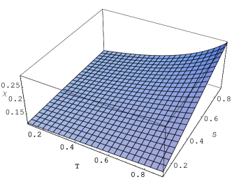
Figure 1: The capacity when $\overline{n}=0.2$.

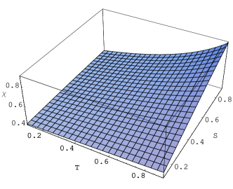
Figure 2: The capacity when $\overline{n}=0.8$.

Examining these diagrams in Figs. 1&2, we can see that the channel capacity always increases with the input signal $\overline{n}$, $T$ and $s$. This is comprehensive, since the noise intensity decreases with larger $T$ and $s$. Meanwhile, $s$ represents how highly entangled $\rho_{AB}$ is. We observe that larger $s$ gives rise to larger channel capacity. So it can be inferred that to gain high channel capacity, the more entangled $\rho_{AB}$ is, the better.

In addition, the fidelity measures the similarity between the input state and the output state. And from the view of quantum information theory, it evaluates how well the channel preserves the transmitted information chuang ; preskill . Thus the fidelity is an important characteristic of quantum channels and a nontrivial quantity to study.

For the input state $\left|\alpha\right\rangle\left\langle\alpha\right|$, the channel fidelity $F$ can be derived as

$$F \equiv \left\langle\alpha\right|\rho_{out}\left|\alpha\right\rangle$$ (9)

$$= \left\langle\alpha\right|\frac{1}{1+\overline{n}_{s}}:e^{-\left(\frac{1}{1+\overline{n}_{s}}+1\right)\left(a^{+}-\alpha^{\ast}\right)\left(a-\alpha\right)}:\left|\alpha\right\rangle$$

$$= \frac{1}{1+\overline{n}_{s}}\times e^{-\left(\frac{1}{1+\overline{n}_{s}}+1\right)\left(\alpha^{\ast}-\alpha^{\ast}\right)\left(\alpha-\alpha\right)}$$

$$= \frac{1}{1+\overline{n}_{s}}$$

For a better understanding, the channel fidelity is plotted as in Fig. 3.

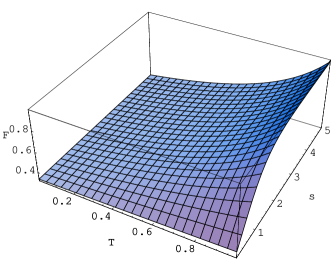
Figure 3: The channel fidelity $F$.

Obviously the channel fidelity $F$ decreases with noise $\overline{n}_{s}$. This is intuitive: The quantum state being transmitted in the channel will become more distorted when the channel is more noisy. Specifically, the channel fidelity increases with $T$ and $s$. As $s$ represents how highly entangled $\rho_{AB}$ is, we can see that the more entangled $\rho_{AB}$ is, the larger the channel fidelity $F$ is.

On the other hand, the channel fidelity here is independent of input signal $\overline{n}$, viz., the mean photon number. This is not always the case. If the bosonic channel is lossy, the channel fidelity decreases with the input signal $\overline{n}$ qin . Therefore, it can be concluded that the channel fidelity is independent of input signal when the channel is not lossy.

In conclusion, we employ the method in Refs. macchi ; qin to examine the properties of continuous variable quantum teleportation. The exact classical capacity of the continuous variable teleportation is given. We find that the channel capacity $\chi$ increases with mean photon number of the input state, and decreases with the growing intensity of the noise. The channel capacity is closely related to the entangled state preshared by Alice and Bob. The more highly entangled $\rho_{AB}$ is, the larger the channel capacity is.

Furthermore, we give the exact channel fidelity in the case when the input state is the coherent state. As expected, the fidelity drops off when the channel becomes more noisy. And surprisingly the channel fidelity is independent of the input mean photon number. The fidelity share the similar properties of the channel capacity. The more entangled $\rho_{AB}$ is, the larger the channel fidelity is.

The scenario we study here can be extended to more complex cases when different input states other than coherent state, such as the squeezed coherent states are considered. Hopefully more interesting outcomes can be obtained.

Noticeably, the method to derive for channel capacity and fidelity in this Letter can be applied to the cases for continuous variable quantum dense coding dense ; kimbledense and continuous variable quantum swapping swapping . Both continuous variable dense coding and swapping can be treated as quantum bosonic channels and they share resembled formulations as continuous variable teleportation does. By making use of the same method in this Letter, similar results will be expected.

Teleportation plays an important role in quantum information theory. We hope our results can stimulate more interest on this subject.

References

- (1) Charles H. Bennett, Gilles Brassard, Claude Crépeau, Richard Jozsa, Asher Peres, and William K. Wootters, Phys. Rev. Lett. 70, 1895 (1993).
- (2) M. Nielson and I. Chuang, Quantum Computation and Quantum Information, Cambridge (2000).
- (3) John Preskill, http://www.theory.caltech.edu/~preskill/ph229
- (4) S. L. Braunstein and A. K. Pati, Quantum Information Theory with Continuous Variables, Dordrecht: Kluwer (2002).
- (5) Garry Bowen and Sougato Bose, Phys. Rev. Lett. 87, 267901 (2001).
- (6) Lev Vaidman, Phys. Rev. A 49, 1473 (1994).
- (7) Dik Bouwmeester, Jian-Wei Pan, Klaus Mattle, Manfred Eibl, Harald Weinfurter, Anton Zeilinger, Nature 390, 575 (1997).
- (8) A. Furusawa, J. L. Sørensen, S. L. Braunstein, C. A. Fuchs, H. J. Kimble, and E. S. Polzik, Science 282, 706 (1998).
- (9) C. W. Gardiner and P. Zoller, Quantum Noise, Springer (2000).
- (10) Thomas M. Cover and Joy A. Thomas, Elements of Information Theory, Wiley-Interscience (1991).
- (11) S. L. Braunstein and H. J. Kimble, Phys. Rev. Lett. 80, 869 (1998)
- (12) Samuel L. Braunstein and Peter van Loock, Rev. Mod. Phys. 77, 513 (2005).
- (13) Masashi Ban, Masahide Sasaki and Masahiro Takeoka, J. Phys. A: Math. Gen. 35, L401 (2002).
- (14) Masahiro Takeoka, Masashi Ban and Masahide Sasaki, J. Opt. B: Quantum Semiclass. Opt. 4, 114 (2002).
- (15) M. Takeoka, M. Sasaki, and M. Ban, Opt. Spectrosc. 94, 675 (2003).
- (16) Ban Masashi, J. Opt. B: Quantum Semiclass. Opt. 6, 224 (2004).
- (17) Stefano Pirandola, Stefano Mancini, and David Vitali, Phys. Rev. A 71, 042326 (2005).
- (18) C. H. Bennett and P. W. Shor, IEEE Trans. Inf. Theory 44, 2724 (1998); A. S. Holevo, Tamagawa Univ. Res. Rev. 4 (1998), quant-ph/9809023.
- (19) A. S. Holevo, IEEE Trans. Inf. Theory 44 269 (1998); P. Hausladen, R. Jozsa, B. Schumacher, M. Westmoreland, and W. K. Wootters, Phys. Rev. A 54 1869 (1996); B. Schumacher and M. D. Westmoreland, ibid. 56 131 (1997).
- (20) Nicolas J. Cerf, Julien Clavareau, Chiara Macchiavello, and Jérémie Roland, Phys. Rev. A 72, 042330 (2005).
- (21) Tao Qin, Meisheng Zhao and Yongde Zhang, quant-ph/0512068
- (22) Masashi Ban, J. Opt. B: Quantum Semiclass. Opt. 2, 786 (2000).
- (23) S. L. Braunstein and H. J. Kimble, Phys. Rev. A 61, 042302 (2000)
- (24) Masashi Ban, J. Phys. A: Math. Gen. 37, L385 (2004).