Geometrical aspects of entanglement

Abstract

We study geometrical aspects of entanglement, with the Hilbert–Schmidt norm defining the metric on the set of density matrices. We focus first on the simplest case of two two-level systems and show that a “relativistic” formulation leads to a complete analysis of the question of separability. Our approach is based on Schmidt decomposition of density matrices for a composite system and non-unitary transformations to a standard form. The positivity of the density matrices is crucial for the method to work. A similar approach works to some extent in higher dimensions, but is a less powerful tool. We further present a numerical method for examining separability, and illustrate the method by a numerical study of bound entanglement in a composite system of two three-level systems.

I Introduction

Entanglement is considered to be one of the main signatures of quantum mechanics, and in recent years the study of different aspects of entanglement has received much attention. One approach has been to study the formal, geometrical characterization of entangled states as opposed to non-entangled or separable states Kus01 ; Verstraete02 ; Pittenger03 . In such a geometrical approach the Hilbert–Schmidt metric defines in many ways the natural metric on the space of of physical states. This metric follows quite naturally from the Hilbert space norm, when the quantum description is extended from pure to mixed states, and it is a Euclidean metric on the set of density matrices. For a composite quantum system the separable states form a convex subset of the full convex set of density matrices, and one of the aims of the geometrical approach is to give a complete specification of this set and thereby of the non-separable or entangled states.

The purpose of this paper is to examine some questions related to the geometrical description of entanglement. We focus primarily on the simplest composite systems consisting of two two-level systems ($2\times 2$ system) or two three-level systems ($3\times 3$ system), but examine also some questions relevant for higher dimensions. In the case of two two-level systems the separable states can be fully identified by use of the Peres criterion Peres96 . This criterion states that every separable density matrix is mapped into a positive semidefinite matrix by partial transposition, i.e., by a transposition relative to one of the subsystems. Since also hermiticity and trace normalization is preserved under this operation, the partial transpose of a separable density matrix is a new density matrix.

A non-separable density matrix, on the other hand, may or may not satisfy Peres’ condition. This means that, in general, Peres’ condition is necessary but not sufficient for separability. However, for the special case of a $2\times 2$ system as well as for a $2\times 3$ system the connection is stronger, and the Peres condition is both necessary and sufficient for a density matrix to be separable Horodecki96 . To identify the separable density matrices, and thereby the entangled states, is therefore in these cases relatively simple. In higher dimensions, in particular for the $3\times 3$ system, that is not the case. Peres’ condition is there not sufficient for separability, and the convex subset consisting of all the density matrices that satisfy this condition is larger than the set of separable matrices. This is part of the reason that the identification of the set of separable states in higher dimensions is a hard problem Gurvits03 .

In the present paper we first give, in Sect. 2, a brief introduction to the geometry of density matrices and separable states. As a next step, in Sect. 3 we focus on the geometry of the two-level system and discuss the natural extension of the Euclidean three dimensional Hilbert–Schmidt metric to a four dimensional indefinite Lorentz metric. This indefinite metric is useful for the discussion of entanglement in the $2\times 2$ system, where Lorentz transformations can be used to transform any density matrix to a diagonal standard form in a way which preserves separability and the Peres condition (Sect. 4). By using this standard form it is straightforward to demonstrate the known fact that any matrix that satisfies the Peres condition is also separable.

The transformation to the diagonal standard form is based on an extension of the Schmidt decomposition to the matrix space with indefinite metric. For general matrices such a decomposition cannot be done, but for density matrices it is possible due to the positivity condition. We show in Sect. 5 that the Schmidt decomposition in this form can be performed not only for the $2\times 2$ system, but for bipartite systems of arbitrary dimensions. However, only for the $2\times 2$ system the decomposition can be used to bring the matrices to a diagonal form where separability can be easily demonstrated. In higher dimensions the Schmidt decomposition gives only a partial simplification. This indicates that to study separability in higher dimensions one eventually has to rely on the use of numerical methods Ioannou04 ; Bruss05 ; Horodecki00 ; Doherty02 ; Badziag05 .

In Sect. 6 we discuss a new numerical method to determine separability Dahl06 , and use the method to study entanglement in the $3\times 3$ system. The method is based on a numerical estimation of the Hilbert–Schmidt distance from any chosen density matrix to the closest separable one. We focus particularly on states that are non-separable but still satisfy the Peres condition. These are states that one usually associates with bound entanglement. A particular example of such states is the one-parameter set discussed by P. Horodecki Horodecki97 and extended by Bruss and Peres Bruss00 . We study numerically the density matrices in the neighbourhood of one particular Horodecki state and provide a map of the states in a two dimensional subspace.

II The geometry of density matrices

II.1 The convex set of density matrices

A density matrix $\rho$ of a quantum system has the following properties,

$$\mbox{$$}\rho^{{\dagger}} = \rho\quad\text{hermiticity}$$

$$\rho > 0\quad\text{positivity}$$

$$\text{Tr}\;\rho = 1\quad\text{normalization}$$ (1)

The matrices that satisfy these conditions form a convex set, and can be written in the form

$$\mbox{$$}\rho=\sum_{k}p_{k}\,|\psi_{k}\rangle\langle\psi_{k}|$$ (2)

with $|\psi_{k}\rangle$ as Hilbert space unit vectors and

$$\mbox{$$}p_{k}\geq 0,\quad\sum_{k}p_{k}=1$$ (3)

The coefficient $p_{k}$, for given $k$, can be interpreted as the probability that the quantum system is in the pure state $|\psi_{k}\rangle$. This interpretation depends, however, on the representation (2), which is by no means unique. In particular, the vectors $|\psi_{k}\rangle$ may be chosen to be orthonormal, then they are eigenvectors of $\rho$ with eigenvalues $p_{k}$, and Eq. (2) is called the spectral representation of $\rho$.

The pure states, represented by the one dimensional projections $|\psi\rangle\langle\psi|$, are the extremal points of the convex set of density matrices. That is, they generate all other density matrices, corresponding to mixed states, by convex combinations of the form (2), but cannot themselves be expressed as non-trivial convex combinations of other density matrices.

The hermitian matrices form a real vector space with a natural scalar product, $\text{Tr}(AB)$, which is bilinear in the two matrices $A$ and $B$ and is positive definite. From this scalar product a Euclidean metric is derived which is called the Hilbert–Schmidt (or Frobenius) metric on the matrix space,

$$\mbox{$$}ds^{2}={1\over 2}\,\mathop{\rm Tr}\nolimits((d\rho)^{2})$$ (4)

The scalar product between pure state density matrices $\rho_{1}=|\psi\rangle\langle\psi|$ and $\rho_{2}=|\phi\rangle\langle\phi|$ is

$$\mbox{$$}\mathop{\rm Tr}\nolimits(\rho_{1}\rho_{2})=|\langle\psi|\phi\rangle|^{2}$$ (5)

For an infinitesimal displacement $|d\psi\rangle$ on the unit sphere in Hilbert space the displacement in the matrix space is

$$\mbox{$$}d\rho=|d\psi\rangle\langle\psi|+|\psi\rangle\langle d\psi|$$ (6)

and the Hilbert–Schmidt metric is

$$\mbox{$$}ds^{2}=\langle d\psi|d\psi\rangle-|\langle\psi|d\psi\rangle|^{2}$$ (7)

where we have used that $\mathop{\rm Tr}\nolimits(d\rho)=\langle\psi|d\psi\rangle+\langle d\psi|\psi\rangle=0$. This may be interpreted as a metric on the complex projective space, called the Fubini–Study metric. It is derived from the Hilbert space metric and is a natural measure of distance between pure quantum states, in fact, $ds$ is the infinitesimal angle between rays (one dimensional subspaces) in Hilbert space. Since the Hilbert–Schmidt metric on density matrices is a direct extension of the Hilbert space metric, it is a natural metric for all, both pure and mixed, quantum states.

A complete set of basis vectors $\{J_{a}\}$, in the space of hermitian matrices, can be chosen to satisfy the normalization condition

$$\mbox{$$}\mathop{\rm Tr}\nolimits(J_{a}J_{b})=\delta_{ab}$$ (8)

For $n\times n$ matrices the dimension of the matrix space, and the number of basis vectors, is $n^{2}$. One basis vector, $J_{0}$, can be chosen to be proportional to the identity $\mathbbm{1}$, then the other basis vectors are traceless matrices. A general density matrix can be expanded in the given basis as

$$\mbox{$$}\rho=\sum_{a}\xi_{a}J_{a}$$ (9)

where the coefficients $\xi_{a}$ are real, and the trace normalization of $\rho$ fixes the value of $\xi_{0}$. With the chosen normalization of $J_{0}$ we have $\xi_{0}=1/\sqrt{n}$.

Due to the normalization, the density matrices are restricted to a hyperplane of dimension $n^{2}-1$, shifted in the direction of $J_{0}$ relative to a plane through the origin. The set of density matrices is further restricted by the positivity condition, so it forms a closed, convex set centered around the point $\rho_{0}=J_{0}/\sqrt{n}$. This point corresponds to the maximally mixed state, which has the same probability $\langle\psi|\rho_{0}|\psi\rangle=1/n$ for any pure state $|\psi\rangle$. The geometry is schematically shown in Fig. 1, where the set of density matrices is pictured as the interior of a circle. One should note that the normalization condition in a sense is trivial and can always be corrected for by a simple scale factor. In the discussion to follow we will find it sometimes convenient to give up this constraint. The quantum states can then be viewed as rays in the matrix space, and the positivity condition restricts these to a convex sector (the cone in Fig. 1).

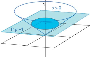
Figure 1: A schematic representation of the set of density matrices in the vector space of hermitian matrices. The positive matrices form a cone about the axis defined by the unit matrix, and the normalization condition restricts the density matrices to a convex subset, here represented by the shaded circle.

II.2 Unitary transformations

The hermitian matrices $J_{a}$ can be viewed as generators of unitary transformations,

$$\mbox{$$}U=\exp\!\left(i\sum_{a}\zeta_{a}J_{a}\right)$$ (10)

with real coefficients $\zeta_{a}$, which act on the density matrices in the following way,

$$\mbox{$$}\rho\rightarrow\tilde{\rho}=U\rho U^{{\dagger}}$$ (11)

If $\rho$ is represented as in Eq. (2), then we see that

$$\mbox{$$}\tilde{\rho}=\sum_{k}p_{k}\,|\tilde{\psi}_{k}\rangle\langle\tilde{\psi}_{k}|$$ (12)

where $|\tilde{\psi}_{k}\rangle=U|\psi_{k}\rangle$. Thus, the matrix transformation $\rho\rightarrow U\rho U^{{\dagger}}$ is induced by the vector transformation $|\psi\rangle\rightarrow U|\psi\rangle$. An immediate consequence of Eq. (12) is that the transformed density matrix $U\rho U^{{\dagger}}$ is positive.

Such unitary transformations respect both the trace and positivity conditions and therefore leave the set of density matrices invariant. Also the von Neumann entropy

$$\mbox{$$}S=-\mathop{\rm Tr}\nolimits(\rho\ln\rho)$$ (13)

is unchanged, which means that the degree of mixing, as measured by the entropy, does not change.

Since the dimension of the set of density matrices grows quadratically with the Hilbert space dimension $n$ the geometry rapidly gets difficult to visualize as $n$ increases. However, the high degree of symmetry under unitary transformations simplifies the picture. The unitary transformations define an $SU(n)$ subgroup of the rotations in the $n^{2}-1$ dimensional matrix space, and all density matrices can be obtained from the diagonal ones by these transformations. In this sense the geometry of the set of density matrices is determined by the geometry of the set of diagonal density matrices. The diagonal matrices form a convex set with a maximal set of $n$ commuting pure states as extremal points. Geometrically, this set is a regular hyperpyramid, a simplex, of dimension $n-1$ with the pure states as corners. The geometrical object corresponding to the full set of density matrices is generated from this by the $SU(n)$ transformations.

In Fig. 2 the set of diagonal density matrices is illustrated for $n=2,3$ and $4$, where in the first case the hyperpyramid has collapsed to a line segment, for $n=3$ it is an equilateral triangle and for $n=4$ it is a tetrahedron. For $n=2$, the $SU(2)$ transformations generate from the line segment the three dimensional Bloch sphere of density matrices. This case is special in the sense that the pure states form the complete surface of the set of density matrices. This does not happen in higher dimensions. In fact, the dimension of the set of pure states is $2n-2$, the dimension of $SU(n)/(U(1)\times SU(n-1))$, because one given pure state has a $U(1)\times SU(n-1)$ invariance group. This dimension grows linearly with $n$, while the dimension of the surface, $n^{2}-2$, grows quadratically.

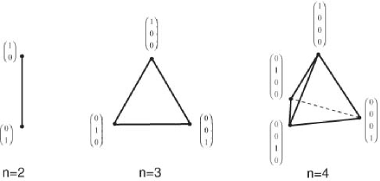
Figure 2: Geometric representation of the diagonal density matrices for the three cases of Hilbert space dimension 1, 2 and 3. For general dimension $n$ they define a hyperpyramid of dimension $n-1$.

The faces of the hyperpyramid of dimension $n-1$ are hyperpyramids of dimension $n-2$, corresponding to density matrices of the subspace orthogonal to the pure state of the opposite corner. Similarly, the hyperpyramid of dimension $n-2$ is bounded by hyperpyramids of dimension $n-3$, etc. This hierarchy is present also in the full set of density matrices, generated from the diagonal ones by $SU(n)$ transformations. Thus, to each extremal point (pure state) the boundary surface opposite to it is a flat face corresponding to the set of density matrices of one lower dimension. In this way the boundary surface of the set of density matrices contains a hierarchy of sets of density matrices of lower dimensions.

The boundary of the set of density matrices is characterized by at least one of the eigenvalues of the density matrices being zero, since outside the boundary the positivity condition is broken. This means that at the boundary the density matrices satisfy the condition $\det\rho=0$, which is an algebraic equation for the coordinates of the boundary points. When $n$ is not too large the equation can be solved numerically. This has been done in Fig. 6 where a two dimensional section of the set of density matrices is shown. One should note that there will be solutions to the equation $\det\rho=0$ also outside the set of density matrices. The boundary of the set of density matrices can be identified as the closed surface, defined by $\det\rho=0$, that encloses the maximally mixed state and is closest to this point.

II.3 More general transformations

We shall later make use of the complex extension of the transformations (10), by allowing $\zeta_{a}$ to be complex. This means that the transformation group is extended from $SU(n)$ to $SL(n,\mathbbm{C})$ (the normalization condition $\det U=1$, or $\zeta_{0}=0$, is trivial). Transformations of the form $\tilde{\rho}=V\rho V^{{\dagger}}$ do not respect the trace condition $\mathop{\rm Tr}\nolimits\rho=1$ if $V$ is non-unitary, but they do respect the positivity condition, because they are still vector transformations of the form (12), with $|\tilde{\psi}_{k}\rangle=V|\psi_{k}\rangle$. This means that they leave the sector of non-normalized density matrices invariant. They no longer keep the entropy unchanged, however. Thus, the larger group $SL(n,\mathbbm{C})$ connects a larger set of density matrices than the restricted group $SU(n)$.

One further generalization is possible. In fact, even if we allow $V$ to be antilinear, the transformation $\tilde{\rho}=V\rho V^{{\dagger}}$ still preserves positivity, because Eq. (12) still holds with $|\tilde{\psi}_{k}\rangle=V|\psi_{k}\rangle$. This point needs some elaboration.

An operator $V$ is antilinear if

$$\mbox{$$}V\,(a\,|\psi\rangle+b\,|\phi\rangle)=a^{\ast}V\,|\psi\rangle+b^{\ast}V\,|\phi\rangle$$ (14)

for any vectors $|\psi\rangle$, $|\phi\rangle$ and complex numbers $a$, $b$. Let $\{|i\rangle\}$ be a set of orthonormal basis vectors, let $\psi_{i}=\langle i|\psi\rangle$ and write $|V\psi\rangle$ for the vector $V\,|\psi\rangle$. Then

$$\mbox{$$}|V\psi\rangle=V\sum_{i}\psi_{i}\,|i\rangle=\sum_{i,j}V_{ji}\psi_{i}^{\ast}\,|j\rangle$$ (15)

with $V_{ji}=\langle j|V|i\rangle$. The hermitian conjugate $V^{{\dagger}}$ is defined in a basis independent way by the identity

$$\mbox{$$}\langle\psi|V^{{\dagger}}\phi\rangle\equiv\langle\phi|V\psi\rangle=\sum_{i,j}\phi_{j}^{\ast}V_{ji}\psi_{i}^{\ast}$$ (16)

or equivalently,

$$\mbox{$$}|V^{{\dagger}}\phi\rangle=V^{{\dagger}}\,|\phi\rangle=\sum_{i,j}\phi_{j}^{\ast}V_{ji}\,|i\rangle$$ (17)

By definition, $V$ is antiunitary if $V^{{\dagger}}=V^{-1}$.

Familiar relations valid for linear operators are not always valid for antilinear operators. For example, when $V$ is antilinear and $|V\psi\rangle=V|\psi\rangle$, it is no longer true that $\langle V\psi|=\langle\psi|V^{{\dagger}}$. This relation cannot hold, simply because $\langle V\psi|$ is a linear functional on the Hilbert space, whereas $\langle\psi|V^{{\dagger}}$ is an antilinear functional. What is nevertheless true is that $V|\psi\rangle\langle\psi|V^{{\dagger}}=|V\psi\rangle\langle V\psi|\;$. In fact, both of these operators are linear, and they act on the vector $|\phi\rangle=\sum_{j}\phi_{j}|j\rangle$ as follows,

$$\mbox{$$}V|\psi\rangle\langle\psi|V^{{\dagger}}|\phi\rangle=V\left(\sum_{i,j}\phi_{j}^{\ast}V_{ji}\psi_{i}^{\ast}|\psi\rangle\right)=\sum_{i,j}\psi_{i}V_{ji}^{\ast}\phi_{j}V\,|\psi\rangle=|V\psi\rangle\langle V\psi|\phi\rangle$$ (18)

As a consequence of this identity the form (12) is valid for the antiunitary transformations, and the positivity is thus preserved.

The transposition of matrices, $\rho\rightarrow\rho^{T}$, obviously preserves positivity, since it preserves the set of eigenvalues. This is not an $SU(n)$ transformation of the form (11), as one can easily check. However, transposition of a hermitian matrix is the same as complex conjugation of the matrix, and if we introduce the complex conjugation operator $K$, which is antilinear and antiunitary, we may write

$$\mbox{$$}\rho^{T}=K\rho K^{{\dagger}}$$ (19)

Note that transposition is a basis dependent operation. The complex conjugation operator $K$ is also basis dependent, it is defined to be antilinear and to leave the basis vectors invariant, $K\,|i\rangle=|i\rangle$. We see that $K^{{\dagger}}=K=K^{-1}$.

One may ask the general question, which are the transformations that preserve positivity of hermitian matrices. If we consider an invertible linear transformation on the real vector space of matrices, then it has to be a one-to-one mapping of the extremal points of the convex set of positive matrices onto the extremal points. In other words, it is a one-to-one mapping of one dimensional projections onto one dimensional projections. In yet other words, it is an invertible vector transformation $|\psi\rangle\rightarrow V|\psi\rangle$, defined up to a phase factor, or more generally an arbitrary non-zero complex factor, for each pure state $|\psi\rangle$. One can show that these complex factors can be chosen in such a way that $V$ becomes either linear or antilinear, and that the matrix transformation is $\rho\rightarrow V\rho V^{{\dagger}}$. However, we will not go into details about this point here.

II.4 Geometry and separability

We consider next a composite system with two subsystems $A$ and $B$, of dimensions $n_{A}$ and $n_{B}$ respectively. By definition, the separable states of the system are described by density matrices that can be written in the form

$$\mbox{$$}\rho=\sum_{k}\,p_{k}\,\rho^{A}_{k}\otimes\rho^{B}_{k}$$ (20)

where $\rho^{A}_{k}$ and $\rho^{B}_{k}$ are density matrices of the two subsystems and $p_{k}$ is a probability distribution over the set of product density matrices labelled by $k$. The separable states form a convex subset of the set of all density matrices of the composite system, with the pure product states $|\psi\rangle\langle\psi|$, where $|\psi\rangle=|\phi\rangle\otimes|\chi\rangle$, as extremal points. Our interest is to study the geometry of this set, and thereby the geometry of the set of entangled states, defined as the complement of the set of separable states within the full set of density matrices.

The Peres criterion Peres96 gives a necessary condition for a density matrix to be separable. Let us introduce orthonormal basis vectors $|i\rangle_{A}$ in ${\cal H}_{A}$ and $|j\rangle_{B}$ in ${\cal H}_{B}$, as well as the product vectors

$$\mbox{$$}|ij\rangle=|i\rangle_{A}\otimes|j\rangle_{B}$$ (21)

We write the matrix elements of the density matrix $\rho$ as

$$\mbox{$$}\rho_{ij;kl}=\langle ij|\rho|kl\rangle$$ (22)

The partial transposition with respect to the $B$ system is defined as the transformation

$$\mbox{$$}\rho\rightarrow\rho^{P}:\quad\rho^{P}_{ij;kl}\equiv\rho_{il;kj}$$ (23)

This operation preserves the trace, but not necessarily the positivity of $\rho$. However, for separable states one can see from the expansion (20) that it preserves positivity, because it is just a transposition of the density matrices $\rho^{B}_{k}$ of the subsystem $B$.

Thus, the Peres criterion states that preservation of positivity under a partial transposition is a necessary condition for a density matrix $\rho$ to be separable. Conversely, if the partial transpose $\rho^{P}$ is not positive definite, it follows that $\rho$ is non-separable or entangled. The opposite is not true: if $\rho^{P}$ is positive, the density matrix $\rho$ is not necessarily separable.

It should be emphasized that the Peres condition, i.e., positivity of both $\rho$ and $\rho^{P}$, is independent of the choice of basis vectors $|i\rangle_{A}$ and $|j\rangle_{B}$. In fact, a change of basis may result in another definition of the partial transpose $\rho^{P}$, which differs from the first one by a unitary transformation, but this does not change the eigenvalue spectrum of $\rho^{P}$. The condition is also the same if transposition is defined with respect to subsystem $A$ rather than $B$. This is obvious, since partial transposition with respect to the $A$ subsystem is just the combined transformation $\rho\rightarrow(\rho^{T})^{P}$.

Let us consider the Peres condition from a geometrical point of view. We first consider the transposition of matrices, $\rho\rightarrow\rho^{T}$, and note that it leaves the Hilbert–Schmidt metric invariant. Being its own inverse, transposition is an inversion in the space of density matrices, or a rotation if the number of inverted directions, $n(n-1)/2$ in an $n\times n$ hermitian matrix, is even. Since $\rho$ and $\rho^{T}$ have the same set of eigenvalues, transposition preserves positivity and maps the set of density matrices onto itself. Thus, the set of density matrices ${\cal D}$ is invariant under transposition as well as under unitary transformations.

Similarly, a partial transposition $\rho\rightarrow\rho^{P}$ preserves the metric and therefore also corresponds to an inversion or rotation in the space of matrices. On the other hand, it does not preserve the eigenvalues and therefore in general does not preserve positivity. This means that the set of density matrices, ${\cal D}$, is not invariant under partial transposition, but is mapped into an inverted or rotated copy ${\cal D}^{P}$. These two sets will partly overlap, in particular, they will overlap in a neighbourhood around the maximally mixed state, since this particular state is invariant under partial transposition. We note that, even though partial transposition is basis dependent, the set of transposed matrices ${\cal D}^{P}$ does not depend on the chosen basis. Nor does it depend on whether partial transposition is defined with respect to subsystem $A$ or $B$.

To sum up the situation, we consider the following three convex sets. ${\cal D}$ is the full set of density matrices of the composite system, while ${\cal P}={\cal D}\cap{\cal D}^{P}$ is the subset of density matrices that satisfy the Peres condition, and ${\cal S}$ is the set of separable density matrices. In general we then have the following inclusions,

$$\mbox{$$}{\cal S}\subset{\cal P}\subset{\cal D}$$ (24)

The Peres criterion is useful thanks to the remarkable fact that partial transposition does not preserve positivity. This fact is indeed remarkable, for the following reason. We have seen that any linear or antilinear vector transformation $|\psi\rangle\rightarrow V|\psi\rangle$ will preserve the positivity of hermitian matrices by the transformation $\rho\rightarrow V\rho V^{{\dagger}}$. It would seem that $V=\mathbbm{1}_{A}\otimes K_{B}$, a complex conjugation on subsystem $B$, would be a vector transformation such that $\rho^{P}=V\rho V^{{\dagger}}$, and hence, that partial transposition would preserve positivity. What is wrong with this argument is that there exists no such operator as $\mathbbm{1}_{A}\otimes K_{B}$. To see why, choose a complex number $c$ with $|c|=1$, and consider the transformation of a product vector $|\psi\rangle=|\phi\rangle\otimes|\chi\rangle$,

$$\mbox{$$}(\mathbbm{1}_{A}\otimes K_{B})|\psi\rangle=(\mathbbm{1}_{A}\otimes K_{B})((c\,|\phi\rangle)\otimes(c^{\ast}\,|\chi\rangle))=c^{2}(|\phi\rangle\otimes(K|\chi\rangle))$$ (25)

The arbitrary phase factor $c^{2}$ invalidates the attempted definition.

The boundary of the congruent (or reflected) image ${\cal D}^{P}$ of ${\cal D}$ is determined by the condition $\det\rho^{P}=0$ in the same way as the boundary of the set of density matrices ${\cal D}$ is determined by $\det\rho=0$. As a consequence, to determine whether a density matrix $\rho$ belongs to the set ${\cal P}$ is not a hard problem. One simply checks whether the determinants of $\hat{\rho}$ and $\hat{\rho}^{P}$ are both positive for every $\hat{\rho}$ on the line segment between $\rho$ and the maximally mixed state $\rho_{0}$. However, to check whether a density matrix is separable and thus belongs to the subset ${\cal S}$ is in general not easy, even though the definition (20) of separability has a simple form. The exceptional cases are the systems of Hilbert space dimensions $2\times 2$, $2\times 3$ or $3\times 2$, where ${\cal S}={\cal P}$.

II.5 Schmidt decomposition and transformation to a standard form

A general density matrix of the composite system can be expanded as

$$\mbox{$$}\rho=\sum_{a=0}^{n_{A}^{2}-1}\sum_{b=0}^{n_{B}^{2}-1}\xi_{ab}\,J^{A}_{a}\otimes J^{B}_{b}$$ (26)

where the coefficients $\xi_{ab}$ are real, and $J^{A}_{a}$ and $J^{B}_{b}$ are orthonormal basis vectors of the two subsystems. We may use our convention that $J^{A}_{0}=\mathbbm{1}_{A}/\sqrt{n_{A}}$ and $J^{B}_{0}=\mathbbm{1}_{B}/\sqrt{n_{B}}$, and that $J^{A}_{k}$ and $J^{B}_{k}$ with $k>0$ are generators of $SU(n_{A})$ and $SU(n_{B})$.

A Schmidt decomposition is a diagonalization of the above expansion. By a suitable choice of basis vectors $\hat{J}^{A}_{a}$ and $\hat{J}^{B}_{b}$, depending on $\rho$, we may always write

$$\mbox{$$}\rho=\sum_{a=0}^{n_{A}^{2}-1}\hat{\xi}_{a}\,\hat{J}^{A}_{a}\otimes\hat{J}^{B}_{a}$$ (27)

assuming that $n_{A}\leq n_{B}$. There exist many different such diagonal representations of a given $\rho$, in fact it is possible to impose various extra conditions on the new basis vectors. It is usual to impose an orthonormality condition, that the new basis vectors should be orthonormal with respect to some positive definite scalar product. Then the Schmidt decomposition of $\rho$ is the same as the singular value decomposition Golub of the $n_{A}^{2}\times n_{B}^{2}$ matrix $\xi_{ab}$. Below, we will introduce a Schmidt decomposistion based on other types of extra conditions.

The usefulness of the representation (27) is limited by the fact that we expand in basis vectors depending on $\rho$. However, we may make a transformation of the form

$$\mbox{$$}\rho\rightarrow\tilde{\rho}=V\rho V^{{\dagger}}$$ (28)

where $V=V_{A}\otimes V_{B}$ is composed of transformations $V_{A}\in SL(n_{A},\mathbbm{C})$ and $V_{B}\in SL(n_{B},\mathbbm{C})$ that act independently on the two subsystems and transform the basis vectors $\hat{J}^{A}_{a}$ and $\hat{J}^{B}_{b}$ into $V_{A}\hat{J}^{A}_{a}V_{A}^{{\dagger}}$ and $V_{B}\hat{J}^{B}_{b}V_{B}^{{\dagger}}$. A transformation of this form obviously preserves the set ${\cal S}$ of separable states, since a sum of the form (20) is transformed into a sum of the same form. It also preserves the set ${\cal P}$ of density matrices satisfying the Peres condition. In fact, it preserves the positivity not only of $\rho$, but also of the partial transpose $\rho^{P}$, since

$$\mbox{$$}(\tilde{\rho})^{P}=(V_{A}\otimes V^{\ast}_{B})\rho^{P}(V_{A}\otimes V^{\ast}_{B})^{{\dagger}}$$ (29)

Here $V^{\ast}_{B}$ is the complex conjugate of $V_{B}$. What is not preserved by the transformation is the trace, but this can easily be corrected by introducing a normalization factor. Such transformations have been considered e.g. by Cen et al. Cen03 .

As we will later show, it is possible to choose the transformation $V=V_{A}\otimes V_{B}$ in such a way that the transformed and normalized density matrix $\tilde{\rho}$ can be brought into the special form

$$\mbox{$$}\tilde{\rho}={1\over n_{A}n_{B}}\left(\mathbbm{1}+\sum_{k=1}^{n_{A}^{2}-1}\tilde{\xi}_{k}\,\tilde{J}^{A}_{k}\otimes\tilde{J}^{B}_{k}\right)$$ (30)

with $\tilde{J}^{A}_{k}$ and $\tilde{J}^{B}_{k}$ as new sets of traceless orthonormal basis vectors. We have some freedom in choosing $V_{A}$ and $V_{B}$, because the form (30) is preserved by unitary transformations of the form $U=U_{A}\otimes U_{B}$.

In the case $n_{A}=n_{B}=2$ we may choose $V_{A}$ and $V_{B}$ so that $\tilde{J}^{A}_{k}$ and $\tilde{J}^{B}_{k}$ are fixed sets of basis vectors, independent of the density matrix $\rho$. In particular, we may use the standard Pauli matrices as basis vectors. In this way we define a special form of the density matrices $\tilde{\rho}$, which we refer to as the standard form. Any density matrix can be brought into this form by a transformation that preserves separability and the Peres condition. All matrices of the resulting standard form commute and can be simultaneously diagonalized. This makes it easy to prove the equality ${\cal S}={\cal P}$, and thereby solve the separability problem. Although this result is well known, the proof given here is simpler than the original proof.

The decomposition (30) is generally valid, but when either $n_{A}$, $n_{B}$, or both are larger than 2, it is impossible to choose both $\tilde{J}^{A}_{k}$ and $\tilde{J}^{B}_{k}$ to be independent of $\rho$. Simply by counting the number of parameters one easily demonstrates that this cannot be done in higher dimensions. Thus, the product transformations $V_{A}\otimes V_{B}$ are specified by $2n_{A}^{2}+2n_{B}^{2}-4$ parameters, while the number of parameters in (30) is $n_{A}^{2}-1$, when the generators $\tilde{J}^{A}_{k}$ and $\tilde{J}^{B}_{k}$ are fixed. This gives a total number of parameters $3n_{A}^{2}+2n_{B}^{2}-5$, when $n_{A}\leq n_{B}$, compared to the number of parameters of the general density matrix, which is $n_{A}^{2}n_{B}^{2}-1$. Only for $n_{A}=n_{B}=2$ do these numbers match.

The mismatch in the number of parameters shows that the independent transformations $V_{A}$ and $V_{B}$ performed on the two subsystems are less efficient in simplifying the form of the density matrices in higher dimensions. In particular, it is impossible to transform all density matrices to a standard form of commuting matrices. Thus, the question of separability is no longer trivially solved. Nevertheless, we consider the Schmidt decomposition to be interesting and important, if only because the number of dimensions in the problem is reduced. We expect this to be useful, even if, at the end, separability can only be determined by numerical methods.

III The two-level system

The density matrices of a two-level system describe the states of a qubit, and represent a simple, but important, special case. It is well known that the normalized density matrices, expressed in terms of the Pauli matrices $\boldsymbol{\sigma}=(\sigma_{1},\sigma_{2},\sigma_{3})$ as

$$\mbox{$$}\rho=\frac{1}{2}\,(\mathbbm{1}+{\bf r}\cdot\boldsymbol{\sigma})$$ (31)

can geometrically be pictured as the interior of a three dimensional unit sphere, the Bloch sphere, with each point identified by a vector ${\bf r}$. The two-level case is special in that the pure states form the complete surface $|{\bf r}|=1$ of the set of density matrices. The diagonal $2\times 2$ matrices, in any chosen basis, correspond to a line segment through the origin with the two pure basis states as end points.

The two-level system is special also in the sense that the Euclidean metric of the three dimensional space of density matrices can be extended in a natural way to an indefinite metric in four dimensions. The extension is analogous to the extension from the three dimensional Euclidean metric to the four dimensional Lorentz metric in special relativity. Since it is useful for the discussion of entanglement in the two qubit system, we shall briefly discussed it here.

We write the density matrix in relativistic notation as

$$\mbox{$$}\rho=\frac{1}{2}\,x^{\mu}\sigma_{\mu}$$ (32)

where $\sigma_{0}$ is the identity matrix $\mathbbm{1}$. The trace normalization condition is that $\mathop{\rm Tr}\nolimits\rho=x^{0}=1$. We may relax this condition and retain only the positivity condition on $\rho$, which means that $x^{0}$ is positive and dominates the vector part ${\bf r}$ of the four-vector $x^{\mu}$, as expressed by the covariant condition

$$\mbox{$$}4\,\det\rho=(x^{0})^{2}-|{\bf r}|^{2}=x^{\mu}x_{\mu}=g_{\mu\nu}x^{\mu}x^{\nu}\geq 0$$ (33)

In other words, the four-vector $x^{\mu}$ is restricted by the positivity condition to be either a time-like vector inside the forward light cone, or a light-like vector on the forward light cone. The light-like vectors correspond to pure states, and the time-like vectors to mixed states. As already discussed, all points on a given line through the origin represent the same normalized density matrix (see Fig. 3).

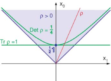
Figure 3: A relativistic view of the density matrices of a two-level system. The positive hermitian matrices are represented by the forward light cone and a density matrix by a time-like or light-like ray (red line). The standard normalization $\mathop{\rm Tr}\nolimits\rho=x^{0}=1$ breaks relativistic invariance (green horizontal line), but may be replaced by the relativistically invariant normalization $\det\rho=x^{\mu}x_{\mu}/4=1/4$ (green hyperbola).

Positivity is conserved by matrix transformations of the form

$$\mbox{$$}\rho\rightarrow\tilde{\rho}=V\rho V^{{\dagger}}=\frac{1}{2}\,L^{\nu}_{\;\;\mu}x^{\mu}\sigma_{\nu}$$ (34)

If we restrict $V$ to be linear (not antilinear), invertible, and normalized by $\det V=1$, then it belongs to the group $SL(2,\mathbbm{C})$, and $L$ is a continuous Lorentz transformation (continuous in the sense that it can be obtained as a product of small transformations). Thus, preservation of positivity by the $SL(2,\mathbbm{C})$ transformations corresponds to preservation of the forward light cone by the continuous Lorentz transformations.

In order to compare the indefinite Lorentz metric to the Euclidean scalar product $\mathop{\rm Tr}\nolimits(AB)$ introduced earlier, we introduce the operation of space inversion,

$$\mbox{$$}\sigma_{\mu}=(\mathbbm{1},\boldsymbol{\sigma})\rightarrow\bar{\sigma}_{\mu}\equiv(\mathbbm{1},-\boldsymbol{\sigma})$$ (35)

It is obtained as a combination of matrix transposition, or equivalently complex conjugation, which for the standard Pauli matrices inverts the sign of $\sigma_{y}=\sigma_{2}$, and a rotation of $\pi$ about the $y$-axis. Thus, for a general hermitian $2\times 2$ matrix $A$ it acts as

$$\mbox{$$}A\rightarrow\bar{A}=RA^{T}R^{{\dagger}}$$ (36)

where

$$\mbox{$$}R=\left(\begin{array}[]{cc}0&-1\\ 1&0\end{array}\right)$$ (39)

We may also write $A^{T}=KAK^{{\dagger}}$, where $K=K^{{\dagger}}$ is complex conjugation.

The Lorentz metric is now expressed by

$$\mbox{$$}\mathop{\rm Tr}\nolimits(\bar{\sigma}_{\mu}\sigma_{\nu})=2g_{\mu\nu}$$ (40)

and the Lorentz invariant scalar product between two hermitian matrices $A=a^{\mu}\sigma_{\mu}$ and $B=b^{\mu}\sigma_{\mu}$ is

$$\mbox{$$}\mathop{\rm Tr}\nolimits(\bar{A}B)=2a^{\mu}b_{\mu}$$ (41)

The invariance of the scalar product (40) can be seen directly from the transformation properties under $SL(2,\mathbbm{C})$ transformations,

$$\mbox{$$}A\rightarrow A^{\prime}=VAV^{{\dagger}}\Rightarrow\bar{A}\rightarrow\bar{A}^{\prime}=V^{{\dagger}-1}\bar{A}V^{-1}$$ (42)

Thus, $A$ and $\bar{A}$ transform under contragredient representations of $SL(2,\mathbbm{C})$.

The Lorentz transformed Pauli matrices

$$\mbox{$$}\tilde{\sigma}_{\mu}=V\sigma_{\mu}V^{{\dagger}}=L^{\nu}_{\;\mu}\sigma_{\nu}\;,\quad V\in SL(2,\mathbbm{C})$$ (43)

satisfy the same metric condition (40) as the standard Pauli matrices $\sigma_{\mu}$. Conversely, any set of matrices $\tilde{\sigma}_{\mu}$ satisfying relations of the form (40) are related to the Pauli matrices by a Lorentz transformation, which need not, however, be restricted to the continuous part of the Lorentz group, but may include space inversion or time reversal, or both.

It is clear from the relativistic representation that any density matrix can be reached from the maximally mixed state $\rho_{0}=\mathbbm{1}/2$ by a transformation corresponding to a boost. The Lorentz boosts generate from $\rho_{0}$ a three dimensional hyperbolic surface (a “mass shell”) where $x^{\mu}x_{\mu}=1$. This surface will intersect any time-like line once and only once. Thus, any mixed state is obtained from $\rho_{0}$ by a unique boost. However, the pure states, corresponding to light-like vectors, can only be reached asymptotically, when the boost velocity approaches the speed of light, here set equal to 1. The form of the $SL(2,\mathbbm{C})$ transformation corresponding to a pure boost is

$$\mbox{$$}V(\boldsymbol{\xi})=\exp\!\left(\frac{1}{2}\,\boldsymbol{\xi}\cdot\boldsymbol{\sigma}\right)$$ (44)

where the three dimensional real vector $\boldsymbol{\xi}$ is the boost parameter, called rapidity. Since the boost matrices are hermitian, a density matrix defined by a boost of the maximally mixed state will have the form

$$\mbox{$$}\rho=N(\xi)V(\boldsymbol{\xi})^{2}=N(\xi)(\cosh\xi\,\mathbbm{1}+\sinh\xi\;\hat{\boldsymbol{\xi}}\cdot\boldsymbol{\sigma})\;,\quad\hat{\boldsymbol{\xi}}=\frac{\boldsymbol{\xi}}{\xi}$$ (45)

where $N(\xi)$ is a normalization factor determined by the trace normalization condition. The normalized density matrix is

$$\mbox{$$}\rho=\frac{1}{2}\,(\mathbbm{1}+\tanh\xi\;\hat{\boldsymbol{\xi}}\cdot\boldsymbol{\sigma})$$ (46)

Thus, the boost parameter $\boldsymbol{\xi}$ gives a representation which is an alternative to the Bloch sphere representation. The relation between the parameters ${\bf r}$ and $\boldsymbol{\xi}$ is that

$$\mbox{$$}{\bf r}=\tanh\xi\;\hat{\boldsymbol{\xi}}$$ (47)

which means that ${\bf r}$ can be identified as the velocity of the boost, in the relativistic picture, with $|{\bf r}|=1$ corresponding to the speed of light. We note that the positivity condition gives no restriction on $\boldsymbol{\xi}$, and the extremal points, i.e.,  the pure states, are points at infinity in the $\boldsymbol{\xi}$ variable.

IV Entanglement in the $2\times 2$ system

We consider now in some detail entanglement between two two-level systems. We will show that with the use of non-unitary transformations the density matrices can be written in a standardized Schmidt decomposed form. In this form the question of separability is easily determined and the equality of the two sets ${\cal P}$ and ${\cal S}$ is readily demonstrated.

IV.1 Schmidt decomposition by Lorentz transformations

We consider transformations $V=V_{A}\otimes V_{B}$ composed of $SL(2,\mathbbm{C})$ transformations acting independently on the two subsystems, and therefore respecting the product form (20) of the separable matrices. We will show that by means of such transformations any density matrix of the composite system can be transformed to the form

$$\mbox{$$}\tilde{\rho}=\frac{1}{4}\left(\mathbbm{1}+\sum_{k=1}^{3}d_{k}\,\sigma_{k}\otimes\sigma_{k}\right)$$ (48)

which we refer to as the standard form. Note that the real coefficients $d_{k}$ must be allowed to take both positive and negative values.

We start by writing a general density matrix in the form

$$\mbox{$$}\rho=c^{\mu\nu}\,\sigma_{\mu}\otimes\sigma_{\nu}$$ (49)

The transformation $V=V_{A}\otimes V_{B}$ produces independent Lorentz transformation $L_{A}$ and $L_{B}$ on the two subsystems,

$$\mbox{$$}\rho\rightarrow\tilde{\rho}=V\rho V^{{\dagger}}=\tilde{c}^{\,\mu\nu}\sigma_{\mu}\otimes\sigma_{\nu}$$ (50)

with

$$\mbox{$$}\tilde{c}^{\,\mu\nu}=L^{\mu}_{A\rho}L^{\nu}_{B\sigma}c^{\rho\sigma}$$ (51)

The Schmidt decomposition consists in choosing $L_{A}$ and $L_{B}$ in such a way that $\tilde{c}^{\,\mu\nu}$ becomes diagonal. We will show that this is always possible when $\rho$ is strictly positive.

Note that the standard Schmidt decomposition, also called the singular value decomposition, involves a compact group of rotations, leaving invariant a positive definite scalar product. The present case is different, because it involves a non-compact group of Lorentz-transformations, leaving invariant an indefinite scalar product.

The positivity condition on $\rho$ plays an essential part in the proof. It states that

$$\mbox{$$}\langle\psi|\rho|\psi\rangle\geq 0$$ (52)

where $|\psi\rangle$ is an arbitrary state vector. Let us consider a density matrix $\rho$ which is strictly positive so that (52) is satisfied with $>$ and not only with $\geq$, and let us restrict $|\psi\rangle$ to be of product form, $|\psi\rangle=|\phi\rangle\otimes|\chi\rangle$. With $\rho$ expressed by (49), the positivity condition then implies

$$\mbox{$$}c^{\mu\nu}m_{\mu}n_{\nu}>0$$ (53)

with

$$\mbox{$$}m_{\mu}=\langle\phi|\sigma_{\mu}|\phi\rangle\;,\quad n_{\nu}=\langle\chi|\sigma_{\nu}|\chi\rangle$$ (54)

These two four-vectors are on the forward light cone, in fact, it is easy to show that

$$\mbox{$$}m_{\mu}m^{\mu}=n_{\mu}n^{\mu}=0\;,\quad m_{0}=n_{0}=1$$ (55)

We note that by varying the state vectors $|\phi\rangle$ and $|\chi\rangle$ all directions on the light cone can be reached. The inequality (53) holds for forward time-like vectors as well, because any such vector may be written as a linear combination of two forward light-like vectors, with positive coefficients. We may actually write a stronger inequality

$$\mbox{$$}c^{\mu\nu}m_{\mu}n_{\nu}\geq C>0$$ (56)

valid for all time-like or light-like vectors $m$ and $n$ with $m_{0}=n_{0}=1$. In fact, this inequality holds because the set of such pairs of four-vectors $(m,n)$ is compact.

Now define the function

$$\mbox{$$}f(m,n)={c^{\mu\nu}m_{\mu}n_{\nu}\over\sqrt{m^{\rho}m_{\rho}\,n^{\sigma}n_{\sigma}}}$$ (57)

It is constant for $m$ and $n$ lying on two fixed, one dimensional rays inside the forward light cone. It goes to infinity when either $m$ or $n$ becomes light-like, because

$$\mbox{$$}f(m,n)\geq{Cm_{0}n_{0}\over\sqrt{m^{\rho}m_{\rho}\,n^{\sigma}n_{\sigma}}}$$ (58)

Using again a compactness argument, we conclude that there exist four-vectors $\bar{m}$ and $\bar{n}$ such that $f(\bar{m},\bar{n})$ is minimal. We may now choose the Lorentz transformations $L_{A}$ and $L_{B}$ such that

$$\mbox{$$}L^{0}_{A\mu}=\bar{m}_{\mu}\;,\quad L^{0}_{B\mu}=\bar{n}_{\mu}$$ (59)

assuming the normalization conditions $\bar{m}^{\mu}\bar{m}_{\mu}=\bar{n}^{\mu}\bar{n}_{\mu}=1$. This defines $L_{A}$ and $L_{B}$ uniquely up to arbitrary three dimensional rotations. Define

$$\mbox{$$}\tilde{f}(m,n)={\tilde{c}^{\,\mu\nu}m_{\mu}n_{\nu}\over\sqrt{m^{\rho}m_{\rho}\,n^{\sigma}n_{\sigma}}}$$ (60)

Since $\tilde{f}(m,n)=f(\tilde{m},\tilde{n})$, with $\tilde{m}_{\mu}=L^{\rho}_{A\mu}m_{\rho}$ and $\tilde{n}_{\mu}=L^{\rho}_{B\mu}n_{\rho}$, it follows that $\tilde{f}(m,n)$ has a minimum at $m=n=(1,0,0,0)$. The condition for an extremum at $m=n=(1,0,0,0)$ is that $\tilde{c}^{\,0k}=\tilde{c}^{\,k0}=0$ for $k=1,2,3$, so that

$$\mbox{$$}\tilde{\rho}=\tilde{c}^{\,00}\,\mathbbm{1}+\sum_{k=1}^{3}\sum_{l=1}^{3}\tilde{c}^{\,kl}\,\sigma_{k}\otimes\sigma_{l}$$ (61)

The coefficient $\tilde{c}^{\,00}$ is the minimum value of $f(m,n)$, and hence positive.

The last term of Eq. (61) can be diagonalized by a standard Schmidt decomposition, and by a further normalization $\tilde{\rho}$ can be brought into the form (30). Finally, a unitary transformation $\tilde{\rho}\rightarrow U\tilde{\rho}U^{{\dagger}}$ of the product form $U=U_{A}\otimes U_{B}$ may be performed, where the unitary matrices $U_{A}$ and $U_{B}$ may be chosen so that $U_{A}\tilde{J}^{A}_{k}U_{A}^{{\dagger}}=\pm\sigma_{k}$ and $U_{B}\tilde{J}^{B}_{k}U_{B}^{{\dagger}}=\pm\sigma_{k}$. This is aways possible, because $SU(2)$ transformations generate the full three dimensional rotation group, excluding inversions. In this way we obtain the standard form (48).

Note that the standard form  (48) of a given density matrix $\rho$ is not unique, because there exists a discrete subgroup of 24 unitary transformations that transform one matrix of this form into other matrices of the same form. This group includes all permutations of the three basis vectors $\sigma_{k}\otimes\sigma_{k}$, as well as simultaneous reversals of any two of the basis vectors. It is the full symmetry group of a regular tetrahedron. If we want to make the standard form unique we may, for example, impose the conditions $d_{1}\geq d_{2}\geq|d_{3}|$, allowing both positive and negative values of $d_{3}$.

IV.2 Density matrices in the standard form

The density matrices of the standard form (48) define a convex subset of lower dimension than the full set of density matrices. It is a three dimensional section of the 15 dimensional set of density matrices, consisting of commuting (simultaneously diagonalizable) matrices. The eigenvalues, as functions of the parameters $d_{k}$ of Eq. (48), are

$$\mbox{$$}\lambda_{1,2}={1\over 4}\,(1\pm(d_{1}-d_{2})+d_{3})\;,\quad\lambda_{3,4}={1\over 4}\,(1\pm(d_{1}+d_{2})-d_{3})$$ (62)

The pure states (with eigenvalues $1,0,0,0$) that are the extremal points of the convex set of commuting matrices are specified by the conditions

$$\mbox{$$}|d_{1}|=|d_{2}|=|d_{3}|=1\;,\quad d_{1}d_{2}d_{3}=-1$$ (63)

There are four such states, corresponding to the four corners of the tetrahedron of diagonal density matrices, and these are readily identified as four orthogonal Bell states (maximally entangled pure states).

We now consider the action of the partial transposition on the tetrahedron of diagonal density matrices. It preserves the standard form, and transforms the coefficients as $d_{1}\rightarrow d_{1},d_{2}\rightarrow-d_{2},d_{3}\rightarrow d_{3}$. Thus it produces a mirror image of the tetrahedron, by a reflection in the $d_{2}$ direction (see Fig. 4). The density matrices of standard form belonging to the set ${\cal P}$, i.e., satisfying the Peres condition that they remain positive after the partial transposition, form an octahedron which is the intersection of the two tetrahedra.

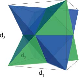
Figure 4: Geometric representation of the diagonal matrices spanned by orthogonal Bell states of the $2\times 2$ system. The density matrices form a tetrahedron (green) while the matrices obtained from this by a partial transposition defines a mirror image (blue). The separable states are defined by the intersection between the two tetrahedra, and forms an octahedron (in the center).

We will now show that for the density matrices of standard form the Peres condition is both necessary and sufficient for separability. What we have to show is that all the density matrices of the octahedron are separable. Since, in general, the separable matrices form a convex set, it is sufficient to show that the corners of the octahedron correspond to separable states.

The density matrices of the octahedron satisfy a single inequality

$$\mbox{$$}|d_{1}|+|d_{2}|+|d_{3}|\leq 1$$ (64)

and its six corners are $(d_{1},d_{2},d_{3})=(\pm 1,0,0),(0,\pm 1,0),(0,0,\pm 1)$, corresponding to the midpoints of the six edges of each of the two tetrahedra. The corners are separable by the identities

$$\mbox{$$}\frac{1}{4}\,(\mathbbm{1}\pm\sigma_{k}\otimes\sigma_{k})={1\over 8}\,[(\mathbbm{1}+\sigma_{k})\otimes(\mathbbm{1}\pm\sigma_{k})+(\mathbbm{1}-\sigma_{k})\otimes(\mathbbm{1}\mp\sigma_{k})]$$ (65)

This completes our proof that the Peres condition is both necessary and sufficient for separability of density matrices on the standard form. Furthermore, since any (non-singular) density matrix can be obtained from a density matrix of standard form by a transformation that preserves both separability and the Peres condition, this reproduces the known result that for the $2\times 2$ system the set of density matrices that remain positive after a partial transposition is identical to the set of separable density matrices.

With this we conclude the discussion of the two-qubit system. The main point has been to show the usefulness of applying the non-unitary Lorentz transformations in the discussion of separability. Also in higher dimensions such transformations can be applied in the form of $SL(n,\mathbbm{C})$ transformations, although not in precisely the same form as with two-level systems.

V Higher dimensions

The relativistic formulation is specific for the two-level system, but some elements can be generalized to higher dimensions. We consider first a single system with Hilbert space dimension $n$. Again, if the trace condition is relaxed, the symmetry group $SU(n)$ of the set of density matrices is extended to $SL(n,\mathbbm{C})$. The Hilbert–Schmidt metric is not invariant under this larger group, but the determinant is invariant for any $n$. However, it is only for $n=2$ that the determinant is quadratic and can be interpreted as defining an invariant indefinite metric.

The generalization to $n>2$ of the Lorentz boosts are the hermitian matrices

$$\mbox{$$}V=V^{{\dagger}}\;,\quad\det V=1$$ (66)

and expressed in terms of the $SU(n)$ generators ${\bf J}$ they have the form

$$\mbox{$$}V=\exp(\boldsymbol{\xi}\cdot{\bf J})$$ (67)

with real group parameters $\boldsymbol{\xi}$. Here ${\bf J}$ and $\boldsymbol{\xi}$ are $n^{2}-1$ dimensional vectors. Any strictly positive density matrix $\rho$ (with $\det\rho>0$) can be factorized in terms of hermitian matrices (67) as

$$\mbox{$$}\rho=NV^{2}=N\,\exp(2\boldsymbol{\xi}\cdot{\bf J})$$ (68)

with the normalization factor

$$\mbox{$$}N={1\over\mathop{\rm Tr}\nolimits\exp(2\boldsymbol{\xi}\cdot{\bf J})}=(\det\rho)^{{1\over n}}$$ (69)

Thus, in the same way as for $n=2$, any strictly positive density matrix can be generated from the maximally mixed state by an $SL(n,\mathbbm{C})$ transformation of the form (67). The boundary matrices, however, which satisfy $\det\rho=0$, cannot be expressed in this way, they can be reached by hermitian transformations only asymptotically, as $|\boldsymbol{\xi}|\rightarrow\infty$. In this limit $N\rightarrow 0$, and therefore $\mathop{\rm Tr}\nolimits V^{2}\rightarrow\infty$ for the non-normalized density matrix $V^{2}$.

V.1 Schmidt decomposition

We now consider a composite system, consisting of two subsystems of dimension $n_{A}$ and $n_{B}$, and assume $\rho$ to be a strictly positive density matrix on the Hilbert space ${\cal H}={\cal H}_{A}\otimes{\cal H}_{B}$ of the composite system. The general expansion of $\rho$ in terms of the $SU(n)$ generators is given by (26). Our objective is to show that by a transformation of the form (28), with $V_{A}\in SL(n_{A},\mathbbm{C})$ and $V_{B}\in SL(n_{B},\mathbbm{C})$, followed by normalization, the density matrix can be transformed to the simpler form (30).

Let ${\cal D}_{A}$ and ${\cal D}_{B}$ be the sets of density matrices of the two subsystems $A$ and $B$. The Cartesian product ${\cal D}_{A}\times{\cal D}_{B}$, consisting of all product density matrices $\rho_{A}\otimes\rho_{B}$ with normalization $\mathop{\rm Tr}\nolimits\rho_{A}=\mathop{\rm Tr}\nolimits\rho_{B}=1$, is a compact set of matrices on the full Hilbert space ${\cal H}$. For the given density matrix $\rho$ we define the following function of $\rho_{A}$ and $\rho_{B}$, which does not depend on the normalizations of $\rho_{A}$ and $\rho_{B}$,

$$\mbox{$$}f(\rho_{A},\rho_{B})={\mathop{\rm Tr}\nolimits\left(\rho\,(\rho_{A}\otimes\rho_{B})\right)\over(\det\rho_{A})^{1/n_{A}}\,(\det\rho_{B})^{1/n_{B}}}$$ (70)

This function is well defined on the interior of ${\cal D}_{A}\times{\cal D}_{B}$, where $\det\rho_{A}>0$ and $\det\rho_{B}>0$. Because $\rho$ is assumed to be strictly positive, we have the strict inequality

$$\mbox{$$}\mathop{\rm Tr}\nolimits\left(\rho\,(\rho_{A}\otimes\rho_{B})\right)>0$$ (71)

and since ${\cal D}_{A}\times{\cal D}_{B}$ is compact, we have an even stronger inequality on ${\cal D}_{A}\times{\cal D}_{B}$,

$$\mbox{$$}\mathop{\rm Tr}\nolimits(\rho\,(\rho_{A}\otimes\rho_{B}))\geq C>0$$ (72)

with a lower bound $C$ depending on $\rho$. It follows that $f\to\infty$ on the boundary of ${\cal D}_{A}\times{\cal D}_{B}$, where either $\det\rho_{A}=0$ or $\det\rho_{B}=0$. It follows further that $f$ has a positive minimum on the interior of ${\cal D}_{A}\times{\cal D}_{B}$, with the minimum value attained for at least one product density matrix $\tau_{A}\otimes\tau_{B}$ with $\det\tau_{A}>0$ and $\det\tau_{B}>0$. For $\tau_{A}$ and $\tau_{B}$ we may use the representation (68), written as

$$\mbox{$$}\tau_{A}=T_{A}^{{\dagger}}T_{A}\;,\qquad\tau_{B}=T_{B}^{{\dagger}}T_{B}$$ (73)

ignoring normalization factors. The matrices $T_{A}\in SL(n_{A},\mathbbm{C})$ and $T_{B}\in SL(n_{B},\mathbbm{C})$ may be chosen to be hermitian, but they need not be, since they may be multiplied from the left by arbitrary unitary matrices. We further write $T=T_{A}\otimes T_{B}$, so that

$$\mbox{$$}\tau_{A}\otimes\tau_{B}=T^{{\dagger}}T$$ (74)

Now define a transformed density matrix

$$\mbox{$$}\tilde{\rho}=T\rho T^{{\dagger}}$$ (75)

and define

$$\mbox{$$}\tilde{f}(\rho_{A},\rho_{B})={\mathop{\rm Tr}\nolimits\left(\tilde{\rho}\,(\rho_{A}\otimes\rho_{B})\right)\over(\det\rho_{A})^{1/n_{A}}\,(\det\rho_{B})^{1/n_{B}}}=f(T_{A}^{{\dagger}}\rho_{A}T_{A}\,,\,T_{B}^{{\dagger}}\rho_{B}T_{B})$$ (76)

This transformed function $\tilde{f}$ has a minimum for

$$\mbox{$$}\rho_{A}\otimes\rho_{B}=(T^{{\dagger}})^{-1}\tau_{A}\otimes\tau_{B}T^{-1}=\mathbbm{1}_{A}\otimes\mathbbm{1}_{B}=\mathbbm{1}$$ (77)

Since $\tilde{f}$ is stationary under infinitesimal variations about the minimum, it follows that

$$\mbox{$$}\mathop{\rm Tr}\nolimits(\tilde{\rho}\;\delta(\rho_{A}\otimes\rho_{B}))=0$$ (78)

for all infinitesimal variations

$$\mbox{$$}\delta(\rho_{A}\otimes\rho_{B})=\delta\rho_{A}\otimes\mathbbm{1}_{B}+\mathbbm{1}_{A}\otimes\delta\rho_{B}$$ (79)

subject to the constraints $\det(\mathbbm{1}_{A}+\delta\rho_{A})=\det(\mathbbm{1}_{B}+\delta\rho_{B})=1$, or equivalently,

$$\mbox{$$}\mathop{\rm Tr}\nolimits(\delta\rho_{A})=\mathop{\rm Tr}\nolimits(\delta\rho_{B})=0$$ (80)

The variations satisfying the constraints are the general linear combinations of the $SU$ generators,

$$\mbox{$$}\delta\rho_{A}=\sum_{i}\delta c^{A}_{i}\,J^{A}_{i}\;,\qquad\delta\rho_{B}=\sum_{j}\delta c^{B}_{j}\,J^{B}_{j}$$ (81)

It follows that

$$\mbox{$$}\mathop{\rm Tr}\nolimits(\tilde{\rho}\;J^{A}_{i}\otimes\mathbbm{1}_{B})=\mathop{\rm Tr}\nolimits(\tilde{\rho}\;\mathbbm{1}_{A}\otimes J^{B}_{j})=0$$ (82)

for all $SU(n_{A})$ generators $J^{A}_{i}$ and all $SU(n_{B})$ generators $J^{B}_{j}$. This means that the terms proportional to $J^{A}_{i}\otimes\mathbbm{1}_{B}$ and $\mathbbm{1}_{A}\otimes J^{B}_{j}$ vanish in the expansion for $\tilde{\rho}$, which therefore has the form

$$\mbox{$$}\tilde{\rho}={1\over{n_{A}n_{B}}}\left(\mathbbm{1}+\sum_{k=1}^{n_{A}^{2}-1}\sum_{l=1}^{n_{B}^{2}-1}\xi_{kl}J^{A}_{k}\otimes J^{B}_{l}\right)$$ (83)

In order to write $\tilde{\rho}$ in the Schmidt decomposed form (30), we have to make a change of basis, from the fixed basis sets $J^{A}_{i}$ and $J^{B}_{j}$ to other orthonormal $SU$ generators $\tilde{J}^{A}_{i}$ and $\tilde{J}^{B}_{j}$ depending on $\tilde{\rho}$. This final Schmidt decomposition involves a standard singular value decomposition of the matrix $\xi_{kl}$ by orthogonal transformations. We may make further unitary transformations $U=U_{A}\otimes U_{B}$, but as already pointed out, this is in general not sufficient to obtain a standard form independent of $\rho$.

VI Numerical approach to the study of separability

In higher dimensions the Peres condition is not sufficient to identify the separable states. In other words, there exist entangled states that remain positive after a partial transposition. This is known not only from general theoretical considerations Horodecki96 , but also from explicit examples Horodecki97 . States of this type have been referred to as having bound entanglement. However, whereas it is a fairly simple task to check the Peres condition, it is in general difficult to identify the separable states Gurvits03 .

In this section we discuss a general numerical method for identifying separability, previously introduced in Dahl06 . It is based on an iterative scheme for calculating the closest separable state and the distance to it, given an arbitrary density matrix (test state). The method can be used to test single density matrices for separability or to make a systematic search to identify the boundary of the set of separable density matrices. After giving an outline of the method we show how to apply the method in a numerical study of bound entanglement in a $3\times 3$ system.

VI.1 Outline of the method

Assume a test state $\rho$ has been chosen. This may typically be close to the boundary of the set of states that satisfy the Peres condition. Let $\rho_{s}$ be a separable state, an approximation in the iterative scheme to the closest separable state. We may start for example with $\rho_{s}=\mathbbm{1}/n$, the maximally mixed state, or with any pure product state. The direction from $\rho_{s}$ to $\rho$ is denoted $\sigma=\rho-\rho_{s}$. In order to improve the estimate $\rho_{s}$ we look for a pure product state $\rho_{p}$ that maximizes the scalar product

$$\mbox{$$}s=\mathop{\rm Tr}\nolimits((\rho_{p}-\rho_{s})\sigma)$$ (84)

or equivalently, maximizes $s^{\prime}=\mathop{\rm Tr}\nolimits(\rho_{p}\sigma)$ (see Fig. 5).

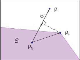
Figure 5: Schematic illustration of the method of finding the separable state closest to a test matrix $\rho$. The matrix $\rho_{s}$ represents the best approximation to the closest separable state at a given step in the iteration, while $\rho_{p}$ is the product matrix that maximizes the scalar product with the matrix $\sigma=\rho-\rho_{s}$. This matrix is used to improve $\rho_{s}$ at the next step in the iteration. The colored area ${\cal S}$ in the figure illustrates a section through the set of separable density matrices.

If $s>0$, then it is possible to find a closer separable state $\rho^{\prime}_{s}$ by mixing in the product state $\rho_{p}$. This search for closer separable states is iterated, either until no pure product state $\rho_{p}$ can be found such that $s>0$, which means that $\rho_{s}$ is already the unique separable state closest to $\rho$, or until some other convergence criterion is satisfied.

There are two separate mathematical subproblems that have to be solved numerically in this scheme. The first problem is to find the pure product state maximizing the scalar product $s^{\prime}$. The second problem is the so called quadratic programming problem: given a finite number of pure product states, to find the convex combination of these which is closest to the given state $\rho$. Our approach to these two problems is described briefly below. We refer to reference Dahl06 for more details.

To approach the first subproblem, note that a pure product state $\rho_{p}$ has matrix elements of the form

$$\mbox{$$}\langle ij|\rho_{p}|kl\rangle=\phi_{i}\chi_{j}\phi_{k}^{\ast}\chi_{l}^{\ast}$$ (85)

where $\sum_{i}|\phi_{i}|^{2}=\sum_{j}|\chi_{j}|^{2}=1$. We want to find complex coefficients $\phi_{i}$ and $\chi_{j}$ that maximize

$$\mbox{$$}s^{\prime}=\mathop{\rm Tr}\nolimits(\rho_{p}\sigma)=\sum_{i,j,k,l}\phi_{i}^{\ast}\,\chi_{j}^{\ast}\,\sigma_{ij;kl}\,\phi_{k}\,\chi_{l}$$ (86)

The following iteration scheme turns out in practice to be an efficient numerical method. It may not necessarily give a global maximum, but at least it gives a useful local maximum that may depend on a randomly chosen starting point.

The method is based on the observation that the maximum value of $s^{\prime}$ is actually the maximal eigenvalue $\mu$ in the two linked eigenvalue problems

$$\mbox{$$}\sum_{k}A_{ik}\,\phi_{k}=\mu\phi_{i}\;,\qquad\sum_{l}B_{jl}\,\chi_{l}=\mu\chi_{j}$$ (87)

where

$$\mbox{$$}A_{ik}=\sum_{j,l}\chi_{j}^{\ast}\,\sigma_{ij;kl}\,\chi_{l}\;,\qquad B_{jl}=\sum_{i,k}\phi_{i}^{\ast}\,\sigma_{ij;kl}\,\phi_{k}$$ (88)

Thus, we may start with any arbitrary unit vector $|\chi\rangle=\sum_{j}\chi_{j}\,|j\rangle_{B}\in{\cal H}_{B}$ and compute the hermitian matrix $A$. We compute the unit vector $|\phi\rangle=\sum_{i}\phi_{i}\,|i\rangle_{A}\in{\cal H}_{A}$ as an eigenvector of $A$ with maximal eigenvalue, and we use it to compute the hermitian matrix $B$. Next, we compute a new unit vector $|\chi\rangle$ as an eigenvector of $B$ with maximal eigenvalue, and we iterate the whole procedure.

This iteration scheme is guaranteed to produce a non-decreasing sequence of function values $s^{\prime}$, which must converge to a maximum value $\mu$. This is at least a local maximum, and there corresponds to it at least one product vector $|\phi\rangle\otimes|\chi\rangle$ and product density matrix $\rho_{p}=(|\phi\rangle\langle\phi|)\otimes(|\chi\rangle\langle\chi|)$.

The above construction of $\rho_{p}$ implies, if $s>0$, that there exist separable states

$$\mbox{$$}\rho^{\prime}_{s}=(1-\lambda)\rho_{s}+\lambda\rho_{p}$$ (89)

with $0<\lambda\leq 1$, closer to $\rho$ than $\rho_{s}$ is. However, it turns out to be very inefficient to search only along the line segment from $\rho_{s}$ to $\rho_{p}$ for a better approximation to $\rho$. It is much more efficient to append the new $\rho_{p}$ to a list of product states $\rho_{pk}$ found in previous iterations, and then minimize

$$\mbox{$$}F=\mathop{\rm Tr}\nolimits\left(\rho-\sum_{k}\lambda_{k}\rho_{pk}\right)^{2}$$ (90)

which is a quadratic function of coefficients $\lambda_{k}\geq 0$ with $\sum_{k}\lambda_{k}=1$. We solve this quadratic programming problem by an adaptation of the conjugate gradient method, and we throw away a given product matrix $\rho_{pk}$ if and only if the corresponding coefficient $\lambda_{k}$ becomes zero when $F$ is minimized. In practice, this means that we may construct altogether several hundred or even several thousand product states, but only a limited number of those, typically less than 100 in the cases we have studied, are actually included in the final approximation $\rho_{s}$.

VI.2 Bound entanglement in the $3\times 3$ system

For the $3\times 3$ system (composed of two three-level systems) there are explicit examples of entangled states that remain positive under a partial transposition. This was first discussed by Horodecki Horodecki97 and then an extended set of states was found by Bruss and Peres Bruss00 . We apply the method outlined above to density matrices limited to a two dimensional planar section of the full set. The section is chosen to contain one of the Horodecki states and a Bell state in addition to the maximally mixed state, and the method is used to identify the boundary of the separable states in this two dimensional plane.

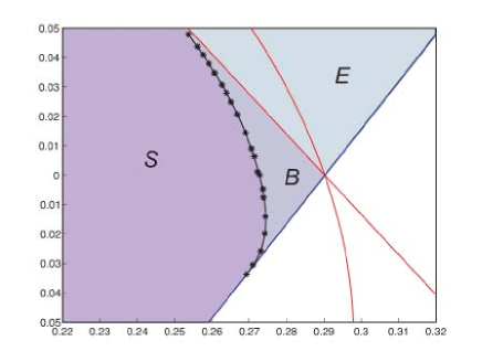
Figure 6: The boundary of the set of separable states in a two dimensional section, as determined by the numerical method. ${\cal S}$ denotes the set of separable states, ${\cal B}$ the states with bound entanglement and ${\cal E}$ the entangled states violating the Peres condition. The blue straight line is determined by the algebraic equation $\det\rho=0$ and gives the boundary of the full set of density matrices. The red curves are determined by the equation $\det\rho_{p}=0$, in particular, the red straight line gives the boundary of the set of states that satisfy the Peres condition. The black dots are the numerically determined points on the boundary of the set of separable states. Note that the coordinates given in this plot differs from the distance defined in the main text by a factor $\sqrt{2}$.

Since the separable states $\cal S$ are contained in the set ${\cal P}$ of states that remain positive under partial transposition, we start the search for the boundary of ${\cal S}$ with a series of states located at the boundary of ${\cal P}$. This boundary is found by solving the algebraic equations $\det\rho=0$ and $\det\rho^{P}=0$. For each chosen state we find the distance to the closest separable state and change the test state $\rho$ on a straight line between this point and the maximally mixed state, in a step of length equal to the evaluated distance. In a small number of steps the intersection of the straight line and the boundary of the separable states is found within a small error, typically chosen to be $10^{-6}$. (The distance from the maximally mixed state to the pure states in this case is $d=2/3$.)

In Fig. 6 we show a plot of the results of the calculations. The numerically determined points on the border of the set of separable states ${\cal S}$ are indicated by black dots, while the border of the set of states ${\cal P}$ that satisfy Peres’ condition, determined by solving the algebraic equations, is shown as blue and red lines which cross at the position of the Horodecki state. One should note that the states with bound entanglement in the corner of the set ${\cal P}$ cover a rather small area.

VII Conclusions

To summarize, we have in this paper focussed on some basic questions concerning the geometry of separability. The simplest case of $2\times 2$ matrices has been used to demonstrate the usefulness of relaxing the normalization requirement $\mathop{\rm Tr}\nolimits\rho=1$. Thus, if this condition is replaced by $\det\rho=1$, a relativistic description with a Minkowski metric can be used, where all (non-pure) states can be connected by Lorentz transformations. For a composite system consisting of two two-level systems, independent Lorentz transformations performed on the two sub-systems can be used to diagonalize an arbitrary density matrix in a way that respects separability. We have used this diagonalization to demonstrate the known fact that the Peres condition and the separability condition are equivalent in this case.

Although the diagonalization with Lorentz transformations is restricted to the composite $2\times 2$ system, we have shown that the generalized form of the Schmidt decomposition used in this diagonalization can be extended to higher dimensions. The decomposition involves the use of non-unitary $SL(n,\mathbb{C})$ transformations for the two subsystems. Although a full diagonalization is not obtained in this way, we suggest that the Schmidt decomposed form may be of interest in the study of separability and bound entanglement.

A third part of the paper has been focussed on the use of a numerical method to study separability. This method exploits the fact that the set of separable states is convex, and is based on an iterative scheme to find the closest separable state for an arbitrary density matrices. We have demonstrated the use of this method in a numerical study of bound entanglement in the case of a $3\times 3$ system. A further study of separability with this method is under way.

Acknowledgments

We acknowledge the support of NorForsk under the Nordic network program Low-dimensional physics: The theoretical basis of nanotechnology. One of us (JML) would like to thank Prof. B. Janko at the Institute for Theoretical Sciences, a joint institute of University of Notre Dame and the Argonne Nat. Lab., for the support and hospitality during a visit in the fall of 2005.

References

- (1) M. Kus and K. Zyczkowski, Geometry of entangled states, Phys. Rev. A 63, 032307 (2001).
- (2) F. Verstraete, J. Dehaene and B. De Moor, On the geometry of entangled states, Jour. Mod. Opt. 49, 1277 (2002).
- (3) A.O. Pittinger and M.H. Rubin, Geometry of entanglement witnesses and local detection of entanglement, Phys. Rev. A 67, 012327 (2003).
- (4) A. Peres, Separability Criterion for Density Matrices Phys. Rev. Lett. 77 (1996) 1413.
- (5) M. Horodecki, P. Horodecki and R. Horodecki, Separability of mixed states: necessary and sufficient conditions, Phys. Lett. A 223 (1996) 1.
- (6) L. Gurvits, Classical deterministic complexity of Edmonds problem and quantum entanglement. In Proceedings of the Thirty-Fifth ACM Symposium on Theory of Computing (ACM, New York, 2003), pp. 10-19.
- (7) L. Ioannou, B. Travaglione, D. Cheung, A. Ekert, Improved algorithm for quantum separability and entanglement detection , Phys. Rev. A 70, 060303 (2004).
- (8) F. Hulpke, D. Bruss, A two-way algorithm for the entanglement problem, J. Phys. A:Math. Gen, 38 (2005) 5573
- (9) P. Horodecki, M. Lewenstein, G. Vidal, I. Cirac, Operational criterion and constructive checks for the separability of low rank density matrices, Phys. Rev. A 62, 032310 (2000).
- (10) A.C. Doherty, P.A. Parrilo, F.M. Spedalieri, Distinguishing separable and entangled states, Phys. Rev. Lett. 88, 187904 (2002).
- (11) P. Badzia̧g, P. Horodecki, R. Horodecki, Towards efficient algorithm deciding separability of distributed quantum states, arXiv:quant-ph/0504041 (2005).
- (12) G. Dahl, J.M. Leinaas, J. Myrheim and E. Ovrum, A tensor product matrix approximation problem in quantum physics , University of Oslo, Dept. of Math/CMA, preprint in Pure Mathematics no.3, 2006.
- (13) P. Horodecki, Separability criterion and inseparable mixed states with positive partial transposition, Phys. Lett. A 232, 333 (1997).
- (14) D. Bruss and A. Peres, Construction of quantum states with bound entanglement, Phys. Rev. A 61, 030301 (2000).
- (15) G.H. Golub and C.F. Van Loan, Matrix Computations (North Oxford Academic Publishing, 1986).
- (16) Li-Xiang Cen, Xin-Qi Li and Yi Jing Yan, Characterization of entanglement transformation via group representation theory, J. Phys. A: Math. Gen. 36 12267 (2003).