Geometrical phase of thermal state in hydrogen atom

Abstract

In this paper, the geometric phase of thermal state in hydrogen atom under the effects of external magnetic field is considered. Especially the effects of the temperature upon the geometric phase is discussed. Also we discuss the time evolution of entanglement of the system. They show some similar behaviors.

I Introduction

The concept of geometric phase was first introduced by Panchartnam in his study of interference of classical light in distinct states of polarization pancharatnam . Berry’s work showed a quantum pure state can retain the information of its motion when it undergoes a cyclic evolution berry . Simon simon subsequently recasted the mathematical formation of Berry phase with the language of differential geometry and fibre bundles. He observed that the origin of Berry phase is attributed to the holonomy in the parameter space. It has been pointed out that the non-Abelian holonomy may be used in the construction of universal sets of quantum gates for the purpose of achieving fault-tolerant quantum computation zanardi1 ; zanardi2 . The holonomy quantum information processing is vary important due to its robustness to imperfections, such as decoherence and the random unitary perturbations.

For a composite system, the Berry phase will be changed by the intersubsystem couplings. Berry phase can be used to the implementation of quantum computation; all the system for the above purpose are composite. Composite systems have great importance in quantum computation, such as the manipulation of qubits, the construction of entanglement and the realization of logic operations. X.X. Yi et al xxyi studied the Berry phase in a composite system with one driven subsystem and found that the Berry phase for a mixed state $\rho(t)=\sum_{j}p_{j}|E_{j}\rangle\langle E_{j}|$ is the average of the individual Berry phases, weighted by their eigenvalues $p_{j}$.

In the early discussions, most researches were focused on the evolution of pure states. Uhlmann was probably the first to address the issue of mixed state holonomy, but as a purely mathematical problem uhlmann1 ; uhlmann2 . Later Sjöqvist et al discussed the geometric phase for non-degenerate mixed state under unitary evolution in his famous paper sjoqvist , basing on the Mach-Zender interferometer. The holonomy attacked interested due to its potential importance to fault-tolerent quantum information processing. M. Nordling et al introduced the concept of non-Abelian holonomy for adiabatic transport of energetically degenerate mixed quantum states nordling .

Recently Tong, et altong proposed a definition for mixed-state geometric phase which was gauge invariant and applicable to the non-unitary evolution,

$$\gamma_{g}=\arg(\sum_{k=1}^{4}\sqrt{\lambda_{k}(0)\lambda_{k}(t)}\langle k|U(t)|k\rangle e^{-\int_{0}^{t}\langle k(t^{\prime})|\dot{k}(t^{\prime})\rangle dt^{\prime}}).$$ (1)

where $\lambda_{k}(t)$ is the k-th eigenvalue of the density matrix $\rho(t)$. When the Hamiltonian is independent of time, the phase can be reduced into

$$\gamma_{g}=\arg(\sum_{k=1}^{4}\lambda_{k}\langle k|U(t)|k\rangle e^{i\langle k|H|k\rangle t})$$ (2)

in which $U=e^{-iHt}$ and $|k\rangle$ is the eigenstate of the initial density operator.

The connection between geometric phase and entanglement has now drawn much attention. In a recent work, S. Ryu and Y. Hatsugai ryu tried to establish a connection between the lower bound of the von-Neumann entropy and the Berry phase defined for quantum ground states. It has been proved that in the XY spin chains, geometric phase shows scaling behavior in the vicinity of quantum phase transition point slzhu , just like entanglement osterloh . Up to now, the relationship between geometric phase and entanglement is not clear yet.

II Model

In this paper, the thermal state of the hydrogen atom is discussed. As one knows, in the hydrogen atom, the electron spin is coupled to the nuclear spin by the hyperfine interaction. The hyperfine line for the hydrogen atom has a measured magnitude of 1420 MHz in frequency. Some calculation on the basis of first-order perturbation for the magnetic dipole interaction between the electron and nucleus gives contribution to the coupling strength of $\mathbf{I}\cdot\mathbf{S}$ term. Taking account of the effect of an external magnetic field, one can have a model Hamiltonian which is bec

$$H=H_{0}+H_{I}$$ (3)

where

$$H_{0} = J(I_{x}\cdot S_{x}+I_{y}\cdot S_{y}+I_{z}\cdot S_{z}),$$ (4)

$$H_{I} = CS_{z}+DI_{z},$$ (5)

$J$ is the coupling constant. Here we have assumed that the electronic orbital angular momentum $L$ is zero. The parameters $C$ and $D$ are related with external magnetic fields,

$$C=g\mu_{B}B,\ \ D=-\frac{\mu}{I}B.$$

It is obvious that the commutation $[H_{0},H_{I}]\neq 0$.

As we know, for a hydrogen atom, the nucleus and electron has both spin-1/2, $\mathbf{I}=\mathbf{S}=\frac{1}{2}\mathbf{\sigma}$. The nuclear magnetic moment $\mu$ equals $2.793\mu_{N}$ where $\mu_{N}=e\hbar/(2m_{p})$. In general C is much larger than D, $|C/D|\sim m_{p}/m_{e}\approx 2000$, so for most applications D may be neglected. At the same level of approximation the $g$ factor of the electron may be put equal to 2.

In the next sections one can discuss the geometric phase and entanglement for hydrogen atom ${}^{1}H$.

III Geometric Phase

In this section, the geometric phase of mixed states for hydrogen atom will be discussed. One can assume that at the initial time $t=0$, the system is subject to the external magnetic field $\mathbf{B}$, the model is not degenerate. As we know, if the magnetic field is not imposed, the ground state is degenerate. The external fields destroy the degeneracy completely. The initial state is set to be a thermal state,

$$\rho_{0}=\sum_{i=1}^{4}p_{i}|\psi_{i}\rangle\langle\psi_{i}|.$$ (6)

Here $p_{i}=\exp(-\beta E_{i})/Z$ and $Z=Tr\exp\{-\beta H\}$ is the partition function. $\beta=1/(kT)$. In fact,

$$\rho_{0}=e^{-\beta H}/Tre^{-\beta H}.$$ (7)

where $H=H_{0}+H_{I}$.

At that time, the four eigenvalues of the initial Hamiltonian $H$ are $(J\pm 2C)/4$, $(-J\pm\sqrt{C^{2}+J^{2}})/4$. It is obvious that the system is non-degenerate.

At the time t=0+, one can assume that there is a little change of external magnetic fields, the interaction term is now $(1+\epsilon)H_{I}$ and $\epsilon$ is a small constant. The eigenstate of the model will evolve with the time. Now the time evolution matrix becomes $U=e^{-iH^{\prime}t}$, and $H^{\prime}=H_{0}+(1+\epsilon)H_{I}$ which implies that magnetic field jumps to another fixed value at that moment. Then one calculate the geometric phase of thermal states which involve with the time by means of Eq.4. Obviously, the geometric phase is dependent on the external magnetic field, intersubsystem couplings, temperature and the time.

The explicit form of geometric phase is very tedious, one only can study some special cases. Then one can discuss the effects of some parameters upon the geometric phase respectively.

(1). The coupling constant $C$, in fact, the external magnetic field.

When the C approaches zero, i.e., the magnetic field vanishes, the Hamiltonian $H$ and the density matrix $\rho$ is commutative, the density matrix is not changed with the time. Therefore in this case the geometric phase is zero.

For simplicity, we assume at the initial time, J=1, C=1, $\beta=1$. Then one study the time evolution of geometric phase for different coupling C, i.e., for different external magnetic field. Here one only need to study the effect of $\epsilon$ upon the geometric phase. The Fig.1 shows that for the same initial state, the magnetic field changes more, the geometric phase changes fast accordingly.

Figure 1: Hydrogen, for different $\epsilon$.

One can consider a special case in which $\epsilon=-1$, which means at that moment the external magnetic field is disappeared. The geometric phase still evolve with the time. The relationship can be plotted in the Fig.2.

Figure 2: For hydrogen, the external magnetic field is disappeared. $J=1$, $\beta=1$, $C=1$.

(2). The coupling constant $J$.

The Fig.3 shows at certain time $t=1$, if $J=0$, the geometric phase $\gamma_{g}$ vanishes. For $J>0$ and $J<0$, the behaviors are not same. When $J>0$, $\gamma_{g}$ can reach a larger maximum in the process of evolution than the case of $J<0$. Obviously, when $|J|$ approaches infinity, geometric phase is vanishing. It is obvious that in this case,the term $H_{0}$ will dominate the whole Hamiltonian, the density matrix will approaches zero.

Figure 3: For hydrogen atom, geometric phase versus J, when $C=1$, $\beta=1$ at the time $t=1$.

(3). The temperature parameter $T$.

One also can study the the relationship between geometric phase and the temperature at certain time. The results can be plotted in the Fig.4.

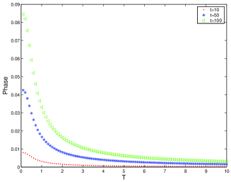
Figure 4: Geometric phase versus temperature at certain time.

From the figure, one can see at certain time, the geometric phase vanishes when the temperature is relatively high. One can see the details in the Fig.5.

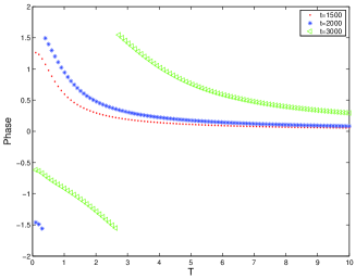
Figure 5: Geometric phase versus temperature.

When the temperature is increased, the system becomes more mixed and disordered. It drivers the geometric phase to approach zero.

IV Concurrence

In the above, we have discussed the time evolution of geometric phase. As we know, entanglement may be created via the interaction of jointed measure, therefore the way in which intersubsystem couplings changes, the geometric phase of a composite system and those of the subsystem is of interest. Here, we shall study the time evolution of entanglement. As we know, for a bi-qubit system, one can use concurrence to measure the entanglement. Speaking briefly, for a bipartite system with the density matrix $\rho$, one can define concurrence

$$\mathfrak{C}=\max\{0,\lambda_{1}-\lambda_{2}-\lambda_{3}-\lambda_{4}\},$$ (8)

where $\lambda_{i}$ is the eigenvalue of the matrix $\sqrt{\rho\sigma_{y}\otimes\sigma_{y}\rho^{\ast}\sigma_{y}\otimes\sigma_{y}}$ and $\lambda_{1}$ is the biggest one. The system is unentangled (maximally entangled) when the concurrence $\mathfrak{C}$ is 0 (1) wootters1 ; wootters2 . Later, the concurrence was used to study the entanglement of the spin chains at finite temperature when the density is the Gibbs density matrix $\rho=e^{-H/kT}/Z$ and $Z=tre^{-H/kT}$ arnesen .

In our work, the density matrix is dependent on the time,

$$\rho(t)=e^{-iHt}\rho_{0}e^{iHt}.$$ (9)

The result is a bit complicated. Fig.6 shows that with the time increasing, the concurrence changes like wave with the time. The entanglement do not vanishes as the time approaches infinity.

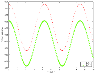
Figure 6: Concurrence versus time at different time.

Fig.7 shows that as the temperature becomes lower, the value of concurrence becomes larger, which implies the system is more entangled at lower temperature. When the temperature is higher than a threshold value, the concurrence vanishes. It implicates that in this case the system is not entangled.

Figure 7: The time evolution of Concurrence versus temperature.

If one compares the properties of the temperature evolution of geometric phase and concurrence respectively, one can see there are some similar properties of them. At certain time, the two both approach zero as the temperature increases. At relatively low temperature, they both decrease with the temperature, which implies there are some relationship between the geometric phase and entanglement. For a relatively large temperature interval, geometric phase is varying very slowly with temperature.

V Summary

We has discussed the time evolution of geometric phase of the hydrogen atom. The relationship between geometric phase and some parameters, such as temperature, external field and coupling constant, has been obtained. We also discussed the time evolution of entanglement. There are some similar properties of their behaviors.

The helpful discussions with Zhe Sun is acknowledged. The work is supported by NSF-China under grant No. 10405019, 10225419 and 90103022.

References

- (1) S. Pacharatnam, Proc. Indian. Acad. Sci. Set. A, 44, 247 (1956).
- (2) M. V. Berry, Proc. R. Soc. London A. 392, 45 (1984).
- (3) B. Simon, Phys. Rev. Lett. 51, 2167 (1983)
- (4) P. Zanardi and M. Rasetti Phys. Lett. A, 264, 94 (1999).
- (5) J. Pachos, P. Zanardi, and M. Rasetti, Phys. Rev. A 61, 010305(R) (2000)
- (6) X.X. Yi, L.C. Wang, and T.Y. Zheng, Phys. Rev. Lett. 92, 150406, (2004).
- (7) A. Uhlmann, Rep. Math. Phys. 24, 229 (1986).
- (8) A. Uhlmann, Lett.Math. Phys. 21, 229 (1991).
- (9) E. Sjöqvist, A. K. Pati, A. Ekert, J. S. Anandan, M. Ericsson, D. K. L. Oi, V. Vedral, Phys. Rev. Lett. 85, 2845 (2000).
- (10) M. Nordling and E. Sjöqvist, Phys. Rev. A, 71, 012110 (2005).
- (11) D. M. Tong, E. Sjöqvist, L. C. Kwek, C. H. Oh, Phys. Rev. Lett. 93, 080405 (2004).
- (12) S. Ryu and Y. Hatsugai, Preprint, cond-mat/0601237.
- (13) S.-L. Zhu, Phys. Rev. Lett. 96, 077206 (2006).
- (14) A. Osterloh, L. Amico, G. Falci, and R. Fazio, Nature, 416, 032110 (2002).
- (15) C. J. Pethick, H. Smith, Bose-Einstein Condensation in Dilute Gases, Cambridge Press, Cambridge, 2002.
- (16) S. Hill and W. K. Wootters, Phys. Rev. Lett. 78 5022,(1997).
- (17) W. K. Wootters, Phys. Rev. Lett. 80, 2245,(1998)
- (18) M. C. Arnesen, S. Bose, V. Vedral, Phys. Rev. Lett. 87 , 017901,(2001).