The Wavefunction of an Anyon

Abstract

We consider a two-dimensional spin system in a honeycomb lattice configuration that exhibits anyonic and fermionic excitations [Kitaev, cond-mat/0506438]. The exact spectrum that corresponds to the translationally invariant case of a vortex-lattice is derived from which the energy of a single pair of vortices can be estimated. The anyonic properties of the vortices are demonstrated and their generation and transportation manipulations are explicitly given. A simple interference experiment with six spins is proposed that can reveal the anyonic statistics of this model.

I Introduction

Lately, a remarkable effort has been made towards the understanding of topological systems (see e.g. Kitaev ; Preskill ; Freedman and references therein). This ranges from the realization of systems that exhibit topological behavior Tsui ; Picciotto ; Xia to the systematic identification and characterization of their topological properties  Kitaev_97 ; Moore ; Read ; Slingerland ; Cooper ; Doucot ; Freedman . These efforts have been greatly boosted by an interest in performing error-free quantum computation Kitaev_97 ; Freedman1 . The idea is to take advantage of the non-trivial statistical properties of anyonic particles, that deviate from the bosonic or fermionic behavior, in order to encode and process information. In these systems, quantum computation is protected from any local errors that do not destroy the nature of the anyons.

This article considers in detail a specific two dimensional lattice model presented by Kitaev Kitaev . It comprises of spin-1/2 particles in a honeycomb configuration that are subject to nearest neighbor interactions. The corresponding quadratic Hamiltonian has been solved analytically in the vortex-free sector and a perturbation treatment was given for its vortex sector Kitaev . Here we present a non-perturbative study of the vortex-lattice sector. The latter consists of vortices placed at each hexagonal plaquette of the lattice. From these analytic results one can estimate the spectrum of two individual vortices in the limit that the interactions between vortices are negligible. Our findings are supported by numerical diagonalization of a small lattice system with 16 spins. A detailed presentation is given of the manipulation procedures required to generate or transport the anyons. The considered system can be employed to perform robust quantum computation with abelian anyons Pachos .

This article is organized as follows. In Section II we present the model and the symmetry properties that enable its analytic treatment. In Section III the separation of the spectrum into different vortex sectors is presented and the properties of anyonic vortices are elaborated. The particular cases of the vortex-free and vortex-lattice sectors are considered and their spectrum is explicitly derived. In the conclusions, the properties of the spectrum are analyzed and an exact numerical treatment is presented that supports our findings. Finally, a minimal lattice cell with six spins is presented that supports anyonic excitations. A simple interference setup is proposed that can reveal the anyonic statistics experimentally.

II Presentation of the model

Consider a two dimensional system with spin-1/2 particles located at the vertices of a honeycomb lattice Kitaev . The spins are assumed to interact with each other via the following Hamiltonian

$$H=-J_{x}\sum_{\text{x-links}}\sigma_{j}^{x}\sigma_{k}^{x}-J_{y}\sum_{\text{y-links}}\sigma_{j}^{y}\sigma_{k}^{y}-J_{z}\sum_{\text{z-links}}\sigma_{j}^{z}\sigma_{k}^{z},$$ (1)

where “x-links”, “y-links” and “z-links” are depicted in Figure 1. Here we shall adopt periodic boundary conditions although open boundary conditions can be similarly treated. Consider an individual hexagonal plaquette and the corresponding operator

$$\hat{w}_{p}=\sigma_{1}^{x}\sigma_{2}^{y}\sigma_{3}^{z}\sigma_{4}^{x}\sigma_{5}^{y}\sigma_{6}^{z},$$ (2)

where $\sigma^{\alpha}_{i}$ is a Pauli operator at vertex $i$ of the hexagon. This operator commutes with the Hamiltonian, $H$, as well as with the corresponding operators, $\hat{w}_{p^{\prime}}$, of all the other plaquettes. Thus, its eigenvalues, $w_{p}=\pm 1$, are conserved quantities. Hence we can split the Hilbert space in sectors, ${\cal L}_{w}$, characterized by a fixed configuration of $w_{p}$’s and solve for the eigenvalues of the Hamiltonian in each sector. A plaquette with $w_{p}=-1$ corresponds to a vortex with anyonic statistics as we shall see in the following. Here the exact diagonalization of the Hamiltonian will be presented for the limiting cases, where $w_{p}=1$ or $w_{p}=-1$, for all plaquettes, $p$. They correspond to the vortex-free and a regular vortex-lattice configuration, the latter having a vortex at each hexagonal plaquette.

To diagonalize Hamiltonian (1) we rewrite the spin operators in terms of Majorana fermions. The latter are defined as the “real” and “imaginary” parts of usual fermionic operators, $a_{k}$ and $a_{k}^{\dagger}$, in the following way

$$c_{2k-1}\equiv a_{k}+a_{k}^{\dagger},\,\,\,\,\,\,c_{2k}\equiv{a_{k}-a_{k}^{\dagger}\over i}.$$ (3)

The Hermitian operators, $c_{i}$, satisfy the following relations, $c_{i}^{\dagger}=c_{i}$ and $\{c_{i},c_{j}\}=2\delta_{ij}$. Here we introduce the fermionic picture by representing each spin with two fermionic modes, $a_{1}$ and $a_{2}$ in such a way that the no-fermion state represents a spin up and the two-fermion state represents a spin down. There are four Majorana operators that correspond to each spin given by

$$c_{0}=a_{1}+a_{1}^{\dagger}=c,\,\,\,\,\,\,c_{1}={a_{1}-a_{1}^{\dagger}\over i}=b^{x},\,\,\,\,\,\,c_{2}=a_{2}+a_{2}^{\dagger}=b^{y},\,\,\,\,\,\,c_{3}={a_{2}-a_{2}^{\dagger}\over i}=b^{z}.$$ (4)

It is possible to project the full space of states of the two fermions to the physical space ${\cal L}$ of the spin states by employing the projection operator $D=b^{x}b^{y}b^{z}c$, where

$$\left|\,\Psi\right\rangle\in{\cal{L}}\Leftrightarrow D\left|\,\Psi\right\rangle=\left|\,\Psi\right\rangle.$$ (5)

Within the subspace ${\cal L}$ the following identifications hold

$$\sigma^{\alpha}=ib^{\alpha}c,\,\,\,\,\,\,(\alpha=x,y,z),$$ (6)

where $\sigma^{\alpha}$ is a specific representation of the Pauli algebra.

To employ this representation for Hamiltonian (1) we introduce four Majorana fermions $b^{x}_{j}$, $b^{y}_{j}$, $b^{z}_{j}$ and $c_{j}$ for each site $j$. As $[\sigma^{\alpha}_{j},D_{k}]=0$ the diagonalization of Hamiltonian (1) is re-expressed as diagonalization of $H(\!\{\sigma^{\alpha}\})=H(\!\{ib^{\alpha}_{j}c_{j}\})$ accompanied by the constraint $D_{j}\left|\,\Psi\right\rangle=\left|\,\Psi\right\rangle$. With the above transformation we have that $\sigma^{\alpha}_{j}\sigma^{\alpha}_{k}=-i\hat{u}_{jk}c_{j}c_{k}$ with $\hat{u}_{jk}\equiv ib^{\alpha}_{j}b^{\alpha}_{k}$, finally obtaining

$$H={i\over 4}\sum_{j,k}\hat{A}_{jk}c_{j}c_{k},\,\,\,\,\,\,\text{where}\,\,\,\,\,\,\hat{A}_{jk}=\left\{\begin{array}[]{c}2J_{\alpha}\hat{u}_{jk},\\ 0,\end{array}\begin{array}[]{l}\text{if $j$ and $k$ are connected by a link,}\\ \text{otherwise.}\end{array}\right.$$ (7)

Observe that $[H,\hat{u}_{jk}]=0$, $\hat{u}^{\dagger}_{jk}=\hat{u}_{jk}$ and $\hat{u}_{jk}^{2}=1$, hence, one can restrict to an eigenspace of states given by a certain configuration of eigenvalues ($u_{jk}=\pm 1$) of the $\hat{u}_{jk}$ operator. This reduces the diagonalization of Hamiltonian (7) to the diagonalization of the corresponding Hamiltonian, where $\hat{A}_{jk}$ is substituted by a certain configuration $A_{jk}$ obtained by replacing $\hat{u}_{jk}$ with its chosen eigenvalue. Thus, instead of considering the decomposition of the Hilbert space with respect to eigenvalues of $\hat{w}_{p}$ one can consider the decomposition, ${\cal L}_{u}$, with respect to the eigenstates of $\hat{u}_{ij}$. Restricted in the physical subspace ${\cal L}$ the following relation holds

$$\hat{w}_{p}=\prod_{(j,k)\in\,boundary(p)}\hat{u}_{jk}$$ (8)

where the $(j,k)$ links are ordered in a clockwise fashion around the plaquette boundary. However, the operators $\hat{u}_{jk}$ and $D_{j}$ do not commute so the resulting eigenstates, $\left|\,\Psi_{u}\right\rangle$, of the Hamiltonian do not satisfy the constraint (5). This is remedied by the symmetrization

$$\left|\,\Psi_{w}\right\rangle=\prod_{j}\left({1+D_{j}\over 2}\right)\left|\,\Psi_{u}\right\rangle.$$ (9)

Thus, the eigenstates of Hamiltonian (7) have to be symmetrized with the above procedure in order to obtain the physical states that correspond to the vortex configurations of Hamiltonian (1). Obviously this procedure does not affect the eigenvalues of the Hamiltonian.

III Spectrum of Hamiltonian

III.1 Sectors of Hilbert space

As we have seen, it is possible to reduce the full Hilbert space of Hamiltonian (1) to independent subspaces, ${\cal L}_{w}$, that correspond to different eigenvalue configurations of $\hat{w}_{p}$. The subspace with $w_{p}=+1$ for all plaquettes $p$ corresponds to the vortex-free configuration. Diagonalizing Hamiltonian (7) in this subspace will just give a fermionic spectrum with no anyons (vortices) present. Changing the sign of one $u_{jk}$ results in two adjacent plaquettes having $w_{p}=-1$. This configuration corresponds to two vortices placed at these plaquettes. In the absence of external fields these anyonic excitations are static in the sense that they remain there indefinitely. One can perform this change of sign in $u_{jk}$ by simple Pauli rotations of the original spins. Indeed, a $\sigma^{z}$ rotation on a certain spin will cause the generation of two vortices in the adjacent plaquettes, as shown in Figure 1. Hamiltonian (7) can now be diagonalized in this subspace of states which results into a fermionic spectrum. The ground state of each sector corresponds to the pure anyonic configuration without fermions.

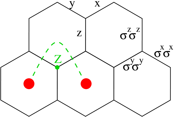
Figure 1: The honeycomb lattice with the three different types of links. At each type corresponds a different spin-spin interaction. Two vortex configuration is induced by a $\sigma^{z}$ rotation at a certain spin. This rotation does not commute with the interaction terms on the $x$- and $y$-links of Hamiltonian (1), a property represented by the dotted connecting string.

To study the vortex excitations as well as their transport properties systematically we shall adopt the operators that correspond to the toric code limit of the model Kitaev ; Pachos obtained, e.g. when $J_{z}\gg J_{x},J_{y}$. In this limit there are three vortex excitations above the ground state, $\left|\,gs\right\rangle$, given by

$$\left|\,Z\right\rangle\equiv\sigma^{z}\otimes 1\left|\,gs\right\rangle\approx 1\otimes\sigma^{z}\left|\,gs\right\rangle,\,\,\,\,\,\,\left|\,Y\right\rangle\equiv\sigma^{x}\otimes\sigma^{y}\left|\,gs\right\rangle\approx\sigma^{y}\otimes\sigma^{x}\left|\,gs\right\rangle,\,\,\,\,\,\,\left|\,X\right\rangle\equiv i\sigma^{x}\otimes\sigma^{x}\left|\,gs\right\rangle.$$ (10)

The two operators of the tensor product are acting on the two spins of a certain $z$-link. The $\left|\,Z\right\rangle$ and $\left|\,Y\right\rangle$ excitations behave as bosons with themselves while the $\left|\,X\right\rangle$ excitation is fermionic. The latter can be produced by fusing the $\left|\,Z\right\rangle$ and $\left|\,Y\right\rangle$ particles and its energy is the sum of the energies of the two constituents. Appropriate applications of the Pauli operators result in the transport of the anyonic subspaces around the lattice. All of the excitations behave as anyons with each other with a statistical angle $\theta=\pi/2$ that results from the anticommutation relations of the Pauli operators. Similarly, the fusion properties of the vortices follow from the properties of the Pauli operators, $X\times X=Y\times Y=Z\times Z=1$, $X\times Y=Z$ and permutations, where $1$ is the no-vortex configuration. For general values of the couplings $J_{\alpha}$ these excitations may be accompanied by non-vortex fermions that reside at each sector. This, of course, does not affect the anyonic properties of the vortices. Hence, it is possible to move between different subspaces, ${\cal L}_{w}$, by applying Pauli rotations on the original spins.

The generation and transport properties of the different sectors do not necessarily correspond to the properties of the anyonic excitations without the fermions. In general, a simple $\sigma^{z}$ rotation moves the vortex-free configuration to the one with two vortices, but fermions may also be generated. To guarantee that no unwanted fermions are created one may consider realizing locally a regime for which one coupling is much larger than the other two, e.g. $J_{z}\gg J_{x},J_{y}$. Then the fermionic energy gap is much larger than the anyonic one Pachos , while we can still find Pauli rotations that correspond to the exchange of energy of the order of the anyonic gap. Indeed, a $\sigma^{z}$ rotation of spin $i$ of the initial Hamiltonian (1) results in a two vortex configuration

$$H_{\text{2-v}}=\sigma^{z}_{i}H\sigma^{z}_{i}=H+2J_{x}\sigma^{x}_{i}\sigma^{x}_{j}+2J_{y}\sigma^{y}_{i}\sigma^{y}_{k},$$ (11)

where $(i,j)$ denotes an $x$-link and $(i,k)$ denotes a $y$-link, and, hence it causes an exchange of energy that scales with $J_{x}$ and $J_{y}$. As we shall see in the following, the fermionic excitations are of the order of $J_{z}$. Hence, they are decoupled from the rest of the system and are negligible in manipulations at this energy scale. It is worth noting that diagonalizing Hamiltonian (11) does not give a $\sigma^{z}$ rotated $\left|\,Z\right\rangle$ state (which would correspond to the lowest energy vortex-free configuration) as that state would correspond to a different sector.

III.2 The vortex-free sector

Due to the symmetry of the Hamiltonian we can restrict ourselves to the case of positive couplings $J_{\alpha}$ Kitaev . The simplest configuration of the eigenvalues of $\hat{u}_{jk}$ is given by $u_{jk}=1$ for all links $(j,k)$ of every hexagonal plaquette taken in a clockwise fashion. This configuration is also known as the vortex-free configuration as it gives $w_{p}=1$ for all plaquettes $p$, and can easily be solved by a Fourier transformation.

Figure 2: (a) The effective square lattice of the original honeycomb model. Each cell (filled circle) incorporates two vertices of the original lattice and a $z$-link, while the depicted $x$ and $y$-links have unit length. (b) The vortex-free case where $u_{jk}=+1$ for $(j,k)$ taken clockwise around each plaquette. (c) The vortex-lattice where $u_{jk}=+1$ for all $(j,k)$ oriented clockwise except for the ones that correspond to every other $z$-link in the $x$ direction.

It is convenient to rearrange the lattice in the following way. Let a unit cell include the $(j,k)$ site that corresponds to the $z$-link. Each cell can be represented by an index $s$ while the position of the vertex within the cell (i.e. distinguishing between $j$ and $k$) is represented by an index $\lambda$ (see Figure 2(a)). Thus, the Hamiltonian takes the form

$$H={i\over 4}\sum_{s\lambda,t\mu}A_{s\lambda,t\mu}c_{s\lambda}c_{t\mu}.$$ (12)

As Hamiltonian (12) is translationally invariant we employ Fourier transforms to diagonalize it. Let us define

$$c_{\lambda}(p)={1\over\sqrt{2N}}\sum_{s}e^{-ip\cdot s}c_{s\lambda},\,\,\,\,\,\,A_{\lambda\mu}(p)=\sum_{t}e^{ip\cdot t}A_{0\lambda,t\mu},$$ (13)

where $p_{x,y}\in[-\pi,\pi]$ and the two dimensional vector, $t=(t_{x},t_{y})$, indicates the position of the vertices on the effective square lattice. The Hamiltonian becomes

$$H={i\over 2}\sum_{\lambda\mu}\int d^{2}\!p\,A_{\lambda\mu}c_{\lambda}^{\dagger}(p)c_{\mu}(p)$$ (14)

where $c^{\dagger}_{\lambda}(p)=c_{\lambda}(-p)$, $c_{\lambda}(p)c_{\mu}^{\dagger}(q)+c_{\mu}^{\dagger}(q)c_{\lambda}(p)=\delta_{pq}\delta_{\lambda\mu}$ and

$$iA(p)=\left(\begin{array}[]{cc}0&if(p)\\ -if^{*}(p)&0\end{array}\right),\,\,\,\,\,\,f(p)=2(J_{x}e^{ip_{x}}+J_{y}e^{ip_{y}}+J_{z}).$$ (15)

For $\varphi\equiv\arg(f(p))$ one can introduce the fermionic operators

$$b(p)=\big{(}c_{1}(p)+ie^{i\varphi}c_{2}(p)\big{)}/\sqrt{2},\,\,\,\,\,\,b^{\dagger}(p)=\big{(}c_{1}(-p)-ie^{-i\varphi}c_{2}(-p)\big{)}/\sqrt{2}.$$ (16)

In terms of $b$ the Hamiltonian takes the diagonal form

$$H=\int d^{2}\!p\,|f(p)|\left[b^{\dagger}(p)b(p)-{1\over 2}\right].$$ (17)

The ground state is given by

$$\left|\,gs\right\rangle=\prod_{p}b(p)\left|\,0\right\rangle=\prod_{p}\big{(}c_{1}^{\dagger}(p)+ie^{-i\varphi}c_{2}^{\dagger}(p)\big{)}\left|\,0\right\rangle,$$ (18)

where $\left|\,0\right\rangle$ is the vacuum state of the Majorana operators, $c_{\lambda}(p)$. The overall ground state energy is $E_{gs}=-{1\over 2}\int d^{2}\!p\,|f(p)|$. The first excited state and its energy gap above the ground state are given by

$$\left|\,e_{p_{0}}\right\rangle=b^{\dagger}(p_{0})\left|\,0\right\rangle,\,\,\,\,\,\,\Delta E_{p_{0}}=\min_{p_{0}}|f(p_{0})|.$$ (19)

It is clear that if $|J_{x}|$, $|J_{y}|$, $|J_{z}|$ satisfy

$$|J_{x}|\leq|J_{y}|+|J_{z}|,\,\,\,\,\,\,|J_{z}|\leq|J_{x}|+|J_{y}|,\,\,\,\,\,\,|J_{y}|\leq|J_{z}|+|J_{x}|,$$ (20)

then there exists a $p_{0}$ such that $\Delta E_{p_{0}}=0$, i.e. the gap vanishes (see Figure 3(a)). The excitation spectrum of the operators $b(p_{0})$ corresponds to the fermionic spectrum of this sector ($w_{p}=1$ for all plaquettes, $p$). Assuming that the coupling configuration is not at the borders of the gapless region one can easily verify that in the gapless region there are two distinctive momenta for which the energy gap becomes zero. At these two Fermi points the energy has conical singularities.

Figure 3: (a) The gapped and gapless phases for the vortex-free case. (b) The gapped and gapless phases for the vortex-lattice case. For both plots $J_{x}+J_{y}+J_{z}=1$ where we assume $J_{x},J_{y},J_{z}\geq 0$. For the vortex-free case (a) the inner boundaries are given by the conditions $J_{x}+J_{y}=J_{z}$, $J_{y}+J_{z}=J_{x}$ and $J_{z}+J_{x}=J_{y}$, while for the vortex-lattice (b) the conditions are $J_{x}^{2}+J_{y}^{2}=J_{z}^{2}$, $J_{y}^{2}+J_{z}^{2}=J_{x}^{2}$ and $J_{z}^{2}+J_{x}^{2}=J_{y}^{2}$.

III.3 The vortex-lattice sector

The anyonic spectrum can be obtained by studying the configuration with $w_{p}=-1$ for all $p$. To implement it we consider the particular case where $u_{jk}$ has alternating signs at the $z$-links along the $x$ direction while it is homogeneous in the $y$ direction (see Figure 2(c)). This is sufficient to create $w_{p}=-1$ for all plaquettes $p$ giving rise to a vortex-lattice where a vortex is placed at each hexagonal plaquette.

As the sign of the $z$-links coupling is now alternating compared to the previous vortex-free case, the Hamiltonian in the momentum representation takes the form

$$H={i\over 2}\sum_{\lambda\mu}\int d^{2}\!p\,d^{2}\!p^{\prime}A_{\lambda\mu}(p,p^{\prime})c_{\lambda}(p)c_{\mu}(p^{\prime}),$$ (21)

where $A_{12}(p,p^{\prime})=\delta(p+p^{\prime})M(p)+\delta(p+p^{\prime}+\pi)N(p)$, $\,\,\,\,\,\,M(p)\equiv 2J_{x}e^{ip_{x}}+2J_{y}e^{ip_{y}}$, $N(p)\equiv 2J_{z}$ and $A_{21}=-A_{12}^{*}$. Explicitly we have

$$H={i\over 2}\int\int_{-\pi}^{\pi}dp_{x}dp_{y}\left\{M(p)c_{1}^{\dagger}(p)c_{2}(p)+M^{*}(p)c_{1}(p)c_{2}^{\dagger}(p)+N(p)\left[c_{1}^{\dagger}(p)c_{2}(\tilde{p})+c_{1}(p)c_{2}^{\dagger}(\tilde{p})\right]\right\},$$ (22)

where $p=(p_{x},p_{y})$ and $\tilde{p}=(p_{x}\pm\pi,p_{y})$. As the last term of (22) is repeated twice in the interval $p_{x}\in[-\pi,\pi]$ the Hamiltonian can be rewritten as

$$H={i\over 2}\int_{-\pi/2}^{\pi/2}dp_{x}\int_{-\pi}^{\pi}dp_{y}\left\{M(p)c_{1}^{\dagger}(p)c_{2}(p)+M(\tilde{p})c_{1}^{\dagger}(\tilde{p})c_{2}(\tilde{p})+N(p)\left[c_{1}^{\dagger}(p)c_{2}(\tilde{p})+c_{1}^{\dagger}(\tilde{p})c_{2}(p)\right]\right\}+\text{h.c.}.$$ (23)

To diagonalize the Hamiltonian Verkholyak we would like to transform (23) into the following form

$$H={i\over 2}\int_{-\pi/2}^{\pi/2}dp_{x}\int_{-\pi}^{\pi}dp_{y}\left[A(p)\eta_{1}^{\dagger}(p)\eta_{2}(p)+B(p)\eta_{1}^{\dagger}(\tilde{p})\eta_{2}(\tilde{p})\right]+\text{h.c.}.$$ (24)

The corresponding canonical transformation has to satisfy

$$[H,\eta_{1}^{\dagger}(p)]=-{i\over 2}A^{*}(p)\eta_{2}^{\dagger}(p),\,\,\,\,\,\,[H,\eta_{1}^{\dagger}(\tilde{p})]=-{i\over 2}B^{*}(p)\eta_{2}^{\dagger}(\tilde{p}),\,\,\,\,\,\,[H,\eta_{2}^{\dagger}(p)]={i\over 2}A(p)\eta_{1}^{\dagger}(p),\,\,\,\,\,\,[H,\eta_{2}^{\dagger}(\tilde{p})]={i\over 2}B(p)\eta_{1}^{\dagger}(\tilde{p}).$$

One can verify that the appropriate transformation is given by

$$c_{\lambda}(p)=\cos\theta\eta_{\lambda}(p)-\sin\theta e^{-(-1)^{\lambda}i\phi}\eta_{\lambda}(\tilde{p}),$$

$$c_{\lambda}(\tilde{p})=\sin\theta e^{(-1)^{\lambda}i\phi}\eta_{\lambda}(p)+\cos\theta\eta_{\lambda}(\tilde{p}),$$ (25)

where $\phi=\arg(M(p)+M^{*}(\tilde{p}))$ and

$$\tan 2\theta={2|M(p)+M^{*}(\tilde{p})|N\over|M(p)|^{2}-|M(\tilde{p})|^{2}}.$$ (26)

The coefficients $A(p)$ and $B(p)$ of Hamiltonian (24) are given by

$$A(p)={|M(p)|^{2}+|M(\tilde{p})|^{2}+2M(p)M(\tilde{p})+\sqrt{\Delta}\over M^{*}(p)+M(\tilde{p})}$$

$$B(p)={|M(p)|^{2}+|M(\tilde{p})|^{2}+2M(p)M(\tilde{p})-\sqrt{\Delta}\over M(p)+M^{*}(\tilde{p})},$$ (27)

where

$$\Delta=\big{(}|M(p)|^{2}-|M(\tilde{p})|^{2}\big{)}^{2}+|M(p)+M^{*}(\tilde{p}))|^{2}N^{2}.$$ (28)

Finally, the Hamiltonian can be diagonalized by employing the following fermionic operators

$$b(p)=\big{(}\eta_{1}(p)+ie^{i\varphi}\eta_{2}(p)\big{)}/\sqrt{2},\,\,\,\,\,\,\,\,\,\,\,\,b(\tilde{p})=\big{(}\eta_{1}(\tilde{p})+ie^{i\varphi^{\prime}}\eta_{2}(\tilde{p})\big{)}/\sqrt{2},$$

$$b^{\dagger}(p)=\big{(}\eta^{\dagger}_{1}(p)-ie^{-i\varphi}\eta^{\dagger}_{2}(p)\big{)}/\sqrt{2},\,\,\,\,\,\,b^{\dagger}(\tilde{p})=\big{(}\eta^{\dagger}_{1}(\tilde{p})-ie^{-i\varphi^{\prime}}\eta^{\dagger}_{2}(\tilde{p})\big{)}/\sqrt{2}.$$ (29)

where $\varphi=\arg(A(p))$ and $\varphi^{\prime}=\arg(B(p))$, eventually giving

$$H=\int_{-\pi/2}^{\pi/2}dp_{x}\int_{-\pi}^{\pi}dp_{y}\left[|A|b^{\dagger}(p)b(p)+|B|b^{\dagger}(\tilde{p})b(\tilde{p})-{|A|+|B|\over 2}\right].$$ (30)

The ground state with its energy is given by

$$\left|\,\text{gs}\right\rangle=\prod_{-\pi/2<q<\pi/2}b(q)b(\tilde{q})\left|\,0\right\rangle,\,\,\,\,\,\,E^{\text{v-l}}_{\text{gs}}=-\int_{-\pi/2}^{\pi/2}dp_{x}\int_{-\pi}^{\pi}dp_{y}{|A|+|B|\over 2},$$ (31)

while some of the first excited states with their energy gap are given by

$$\left|\,e_{p_{0}}\right\rangle=b^{\dagger}(p_{0})\left|\,\text{gs}\right\rangle,\,\,\,\,\,\,\Delta E_{p_{0}}=\min_{p_{0}}|A(p_{0})|,$$

$$\left|\,e_{\tilde{p}_{0}}\right\rangle=b^{\dagger}(\tilde{p}_{0})\left|\,\text{gs}\right\rangle,\,\,\,\,\,\,\Delta E_{\tilde{p}_{0}}=\min_{p_{0}}|B(\tilde{p}_{0})|.$$ (32)

It is possible to derive the values of the couplings for which the vortex-lattice configuration becomes gapless. Note first that $|A(p)|$ cannot be zero, but $|B(p)|$ can. Indeed, there exists $p$ such that $|B(p)|=0$ if and only if all of the conditions below are satisfied

$$J_{x}^{2}+J_{y}^{2}\geq J_{z}^{2},\,\,\,\,\,\,J_{y}^{2}+J_{z}^{2}\geq J_{x}^{2},\,\,\,\,\,\,J_{z}^{2}+J_{x}^{2}\geq J_{y}^{2},$$ (33)

which is given schematically in Figure 3(b). When (33) is satisfied and for coupling configurations away from the borders of the gapless region one can verify that there are two distinctive momenta for which the energy gap becomes zero. At these two Fermi points the energy has conical singularities.

IV Conclusions

As we have seen, vortices with respect to the $u_{jk}$ gauge field have anyonic statistics and are generated in the system by applying proper spin rotations. They are connected either with other vortices, or, when the system is open, with its boundary by string operators. The vortex excitations are static, but they can be transported by applying external fields. Each vortex configuration is accompanied by a fermionic spectrum. We evaluated this spectrum for the limiting cases of the vortex-free and the vortex-lattice configurations. Their ground states are fermionic vacua (pure anyons) from which one can obtain the physical wavefunctions by performing symmetrization (9).

It is of interest to study the behavior of the energy of these configurations as functions of the couplings $J_{\alpha}$. When $J_{x}=J_{y}=0$ then $E^{\text{v-f}}_{\text{gs}}=E^{\text{v-l}}_{\text{gs}}=-J_{z}N$ where $N$ is the total number of plaquettes for both the vortex-free and the vortex-lattice configurations. It is possible to check that for all other values of the couplings $J_{\alpha}$ we have $E^{\text{v-f}}_{\text{gs}}\leq E^{\text{v-l}}_{\text{gs}}$. Hence, the energy minimum is achieved by the vortex-free configuration, a fact that also follows from a theorem by Lieb Lieb and has been verified numerically by Kitaev Kitaev . It is easily observed that the two energies become equal only when one of the couplings $J_{\alpha}$ becomes zero.

One can compare the fermionic excitation energy of the vortex-free configuration with the energy gap of a pair of vortices. To derive the energy of this pair from the energy of the vortex-lattice we assume that the vortices are non-interactive. This assumption is valid in the gapped regime where any interaction mediated by the fermions is exponentially suppressed comment . This is also supported by exact numerical diagonalization as we see in the following. In Figure 4(a) the energy gap is plotted between the ground state and the anyonic or the fermionic excitations. One can easily see that there is a transition in the character of the first excitation from anyonic to fermionic.

(a)

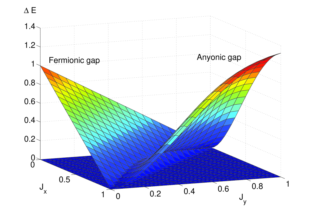
(b)

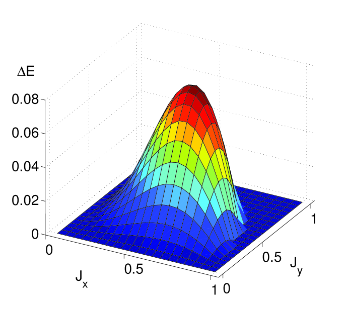
Figure 4: (a) Analytic results for the energy of a pair of anyons and of a fermionic excitation. The anyonic and fermionic energy gaps are plotted against $J_{x}$ and $J_{y}$ where we have set $J_{z}=1$. (b) Numerical evaluation of the energy gap of the first excited state above the ground state. This gap is in agreement with the one given as a minimum of the vortex and fermionic gaps as seen in (a).

To verify our findings we simulate the original Hamiltonian with 16 spins in a periodic honeycomb lattice. In Figure 4(b) we plot the energy gap between the ground state and the first excited one against $J_{x}$ and $J_{y}$, while keeping $J_{z}=1$. There we see that the excitation becomes gapless for values of the couplings which agree with the behavior of the vortex and fermionic excitations. Indeed, the energy gap obtained numerically is approximately nested below the analytically obtained energy gaps with a maximum value that agrees well with the value obtained from Figure 4(a).

We conclude by presenting a simple model with six spins that can reveal the anyonic statistics of the excitations experimentally. It consists of one hexagonal plaquette with only the spin interactions that lay on the hexagon (see Figure 5). An anyonic excitation in the plaquette can be produced by a $\sigma^{z}_{6}$ rotation. Its paired anyon is outside our system thus it does not increase the total energy of the system. In order to obtain the anyonic properties one would like to circulate another anyon around it. Even if it is not possible to have two anyons present in this simple model, one can consider anyons outside the system that can circulate the existing anyon by appropriately rotating the six spins. Indeed, performing the operation $S=\sigma^{z}_{1}\sigma^{y}_{2}\sigma^{x}_{3}\sigma^{z}_{4}\sigma^{x}_{5}\sigma^{y}_{6}$ corresponds to a looping trajectory around the anyonic excitation in the plaquette and, thus, it should generate an overall $\pi$ phase factor. Indeed, for the ground state, $\left|\,gs\right\rangle$, and the vortex state, $\left|\,v\right\rangle=\sigma^{z}_{6}\left|\,gs\right\rangle$, this evolution is given by

$$S\left|\,v\right\rangle=S\sigma^{z}_{6}\left|\,gs\right\rangle=-\sigma^{z}_{6}S\left|\,gs\right\rangle=-\sigma^{z}_{6}\left|\,gs\right\rangle=-\left|\,v\right\rangle$$ (34)

The property $S\left|\,gs\right\rangle=\left|\,gs\right\rangle$ is due to the invariance of the ground state under closed loop operations. It is worth noting that $S$ is also the $\hat{w}_{p}$ operator (2) for the single plaquette of our system.

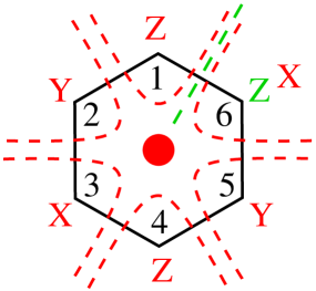
Figure 5: A hexagon that can support anyonic statistics. A vortex is generated, e.g. by a $\sigma^{z}$ rotation of spin $6$. Pauli rotations around the plaquette result in the generation of the looping trajectory. This procedure results in a $\pi$ phase revealing the anyonic statistics of the vortex.

This procedure can be used in an interferometric setup to observe the anyonic statistics experimentally. Indeed, if one performs the rotation $R=(1-i\sigma^{z}_{6})/\sqrt{2}$, then the superposed state $(\left|\,gs\right\rangle-i\left|\,v\right\rangle)/\sqrt{2}$ is produced. The looping evolution and the inverse rotation $R^{-1}$ will result into the $\left|\,v\right\rangle$ state if the statistics of the vortex excitation is anyonic, while a bosonic or fermionic statistics would give back the $\left|\,gs\right\rangle$ state. This interference effect produced with only one hexagonal plaquette can, in principle, be realized with present technology using NMR Glaser or Josephson Junctions Ioffe . Alternatively, one can consider a lattice of vortices where every other vortex is transported around its static neighbor. Such an experiment could be realized in an optical lattice setup with atoms Duan or polar molecules Zoller . The readout of the final configuration could be performed by energy addressing using the spectrum derived in Section III.

- (1) M. Freedman, C. Nayak, K. Shtengel, K. Walker, and Z. Wang, Ann. Phys. 310, 428 (2004).
- (2) A. Kitaev, cond-mat/0506438.
- (3) J. Preskill, Lecture notes on Topological Quantum Computation, http://www.theory.caltech.edu/preskill/ph219/topological.ps.
- (4) D. C. Tsui, H. L. Stormer, and A. C. Gossard, Phys. Rev. Lett. 48, 1559 (1982).
- (5) R. de-Picciotto, et al., Nature 389, 162 (1997).
- (6) J. S. Xia, et al. Phys. Rev. Lett. 93, 176809 (2004).
- (7) A. Kitaev, Annals of Physics 303, 2 (2004).
- (8) G. Moore, and N. Read, Nucl.Phys. B 360, 362 (1991).
- (9) N. Read, and E. Rezayi, Phys. Rev. B 59, 8084 (1999).
- (10) J. K. Slingerland, and F. A. Bais, Nucl. Phys. B 612, 229 (2001).
- (11) N. R. Cooper, N. K. Wilkin, and J. M. F. Gunn, Phys. Rev. Lett. 87, 120405 (2001).
- (12) B. Douçot, L. B. Ioffe, and J. Vidal, Phys. Rev. B 69, 214501 (2004).
- (13) M. Freedman, M. Larsen, and Z. Wang, Comm. Math. Phys. 227, 605 (2002).
- (14) J. K. Pachos, quant-ph/0511273.
- (15) T. Verkholyak, A. Honecker, and W. Brenig, Eur. Phys. J. B 49, 283 287 (2006).
- (16) E. H. Lieb, Phys. Rev. Lett. 73, 2158 (1994).
- (17) In the fermionic gapless phase we expect the anyons to be dressed with fermions that propagate interactions between them and change their energy significantly.
- (18) U. Glaser, H. Büttner, and H. Fehske, Phys. Rev. A 68, 032318 (2003); J. A. Jones, Phys. Rev. A 67, 012317 (2003).
- (19) B. Douçot, M. V. Feigel’man, L. B. Ioffe, and A. S. Ioselevich, Phys. Rev. B 71, 024505 (2005).
- (20) L.-M. Duan, E. Demler, and M. D. Lukin, Phys. Rev. Lett. 91, 090402 (2003).
- (21) A. Micheli, G.K. Brennen, and P. Zoller, quant-ph/0512222.