Creating large noon states with imperfect phase control

Abstract

Optical noon states $(|N,0\rangle+|0,N\rangle)/\sqrt{2}$ are an important resource for Heisenberg-limited metrology and quantum lithography. The only known methods for creating noon states with arbitrary $N$ via linear optics and projective measurments seem to have a limited range of application due to imperfect phase control. Here, we show that bootstrapping techniques can be used to create high-fidelity noon states of arbitrary size.

Introduction

An important part of quantum information processing is quantum metrology and quantum lithography. We speak of quantum—or Heisenberg-limited—metrology when systems in quintessentially quantum mechanical states are used to reduce the uncertainty in a phase measurement below the shot-noise limit. If $\phi$ is the phase to be estimated, and $N$ is the number of independent trials in the estimation, the shot-noise limit is given by $\Delta\phi=1/\sqrt{N}$. In quantum mechanics, the $N$ trials can be correlated such that the limit is reduced to $\Delta\phi=1/N$ Caves (1981); Yurke et al. (1986). It is believed that this is the best phase sensitivity achievable in quantum mechanics.

In optics, $\phi$ may represent the length change in the arm of an interferometer searching for gravity waves. When coherent (laser) light is used, the phase sensitivity is $1/\sqrt{\bar{n}}$, where $\bar{n}$ is the average number of photons in the beam. If, on the other hand, special quantum states of light are used, the phase sensitivity can be improved. One of such states is the so-called noon state:

$$|N::0\rangle_{ab}\equiv\frac{1}{\sqrt{2}}\left(|N,0\rangle_{ab}+|0,N\rangle_{ab}\right).$$ (1)

If one of the modes experiences a phase shift $\phi$, the state becomes $(|N,0\rangle+e^{iN\phi}|0,N\rangle)/\sqrt{2}$. The enhanced phase leads to an increased phase sensitivity of $\Delta\phi=1/N$ Bollinger et al. (1996), which can easily be verified by noting that a phase shift of $\pi/N$ transforms Eq. (1) into an orthogonal state. This means there exists a single-shot experiment that determines the presence or absence of the phase shift.

Another application that requires the ability to create noon states is quantum lithography Boto et al. (2000). Classical light can write and resolve features only with size larger than about a quarter of the wavelength: $\Delta x=\lambda/4$. This is why classical optical lithography is struggling to reach the atomic level. With the use of noon states, however, the minimum resolvable feature size becomes $\Delta x=\lambda/4N$. The same phase enhancement $N\phi$ that gives rise to the Heisenberg limit also enables an unbounded increase in optical resolution Kok et al. (2004). Consequently, noon states have attracted quite some attention in recent years Hofmann (2004); Combes and Wiseman (2005); Pezzé and Smerzi (2005); Sun et al. (2005).

Currently, there are two main procedures for creating noon states: Kerr nonlinearities Gerry (2000), and linear optics with projective measurements Fiurášek (2002); Lee et al. (2002); Kok et al. (2002). Kerr, or optical $\chi^{(3)}$ nonlinearities may in principle yield perfect noon states, but the small natural coupling of $\chi^{(3)}$ and the unavoidable additional transformation channels pose a formidable challenge to any practical implementation. Electromagnetically induced transparencies may be used to solve this problem Schmidt and Imamo$\bar{\rm g}$lu (1996), but even here the creation of noon states needs nonlinearities with appreciably greater strength than what has been demonstrated so far.

All methods for creating large noon states with linear optics and projective measurements use the Fundamental Theorem of Algebra, which states that every polynomial has a factorization (see e.g., Ref. Friedberg et al. (1989)). In particular, the polynomial function of the creation operators that generate a noon state is factorized by the $N$-th roots of unity:

$$\hat{a}^{\dagger N}-\hat{b}^{\dagger N}=\prod_{k=1}^{N}(\hat{a}^{\dagger}+e^{2\pi i(k-1)/N}\,\hat{b}^{\dagger})\;.$$ (2)

Every factor can be implemented probabilistically using beam splitters, phase shifters, and photo-detection Fiurášek (2002); Kok et al. (2002). Three- and four-photon noon states have been demonstrated experimentally by Mitchell et al. Mitchell et al. (2004) and Walther et al. Walther et al. (2004), respectively. In this note, I identify a fundamental problem with the noon-state preparation procedure using linear optics and projective measurements. In addition, I propose a method that can be used to circumvent this problem.

Noisy state preparation

In practice the phase factor $2\pi(k-1)/N$ in Eq. (2) cannot be created with infinite precision. The accuracy of adjusting the phase is bounded by the limits of metrology. In order to create noon states, we must be able to tune the phase shift such that $2\pi(k-1)/N$ and $2\pi k/N$ are well separated. We thus require the phase error to be smaller than $2\pi/N$. This is the Heisenberg limit. If our objective is to create noon states in order to attain the Heisenberg limit, then we encounter a circular argument. This naive line of reasoning therefore suggests that the Heisenberg limit cannot be attained this way. In this note, I quantify the maximum sensitivity using noisy noon states, and explore a possible way to create high-fidelity noon states of arbitrary size.

To estimate the effect of imperfect control over the phase shifts in the preparation process, consider the following noise model. Every phase in every factor of Eq. (2) has a Gaussian distribution with variance $\sqrt{\delta}\,$:

$$\rho = \frac{1}{2N!}\prod_{k=1}^{N}\int\frac{d\varphi_{k}}{\sqrt{2\pi\delta}}\,e^{-(\varphi_{k}-2\pi k/N)^{2}/2\delta}$$ (4)

$$\qquad\times\left(\hat{a}^{\dagger}+e^{i\varphi_{k}}\,\hat{b}^{\dagger}\right)|0\rangle_{ab}\langle 0|\left(\hat{a}+e^{-i\varphi_{k}}\,\hat{b}\right).$$

The variance $\sqrt{\delta}$ is considered sufficiently small such that the integration can be taken over the interval $(-\infty,+\infty)$.

To derive the uncertainty in the phase, we adopt the following measurement model: By virtue of quantum lithography Boto et al. (2000), the noon state can be focussed onto a small region with width $\pi/N$. In this region, a detector measures the observable

$$\hat{\Sigma}=|N,0\rangle_{ab}\langle 0,N|+|0,N\rangle_{ab}\langle N,0|\;.$$ (5)

For a physical model of such a measurement, see Boto et al. Boto et al. (2000). In terms of projection operators, this measurement can be written as

$$\hat{E}_{\pm}=\frac{1}{2}\left(|N,0\rangle\pm|0,N\rangle\right)\left(\langle N,0|\pm\langle 0,N|\right)\;,$$ (6)

and the evolution due to the phase shift yields

$$\rho(\phi)=\left(\mbox{\small 1}\!\!\mbox{1}\otimes e^{i\hat{n}_{b}\phi}\right)\,\rho\,\left(\mbox{\small 1}\!\!\mbox{1}\otimes e^{-i\hat{n}_{b}\phi}\right),$$ (7)

where $\hat{n}_{b}=\hat{b}^{\dagger}\hat{b}$. The conditional probability of finding outcome $j$ in a measurement given a phase shift $\phi$ is then calculated as follows:

$$p(j|\phi)={\rm tr}\left[\hat{E}_{j}\rho(\phi)\right].$$ (8)

The uncertainty in the phase is determined by the Cramér-Rao bound Helstrom (1976):

$$(\Delta\phi)^{2}\geq\frac{1}{F(\phi)}\;,$$ (9)

where $F(\phi)$ is the Fisher information defined by

$$F(\phi)=\sum_{j}\frac{1}{p(j|\phi)}\left[\frac{\partial p(j|\phi)}{\partial\phi}\right]^{2}.$$ (10)

When the input state is a perfect noon state, the Fisher information is $F(\phi)=N^{2}$, and the Cramér-Rao bound yields $\Delta\phi\geq 1/N$. Up to a constant of proportionality, this bound is attained by the measurement procedure outlined above.

When we take into account the Gaussian noise in the state preparation process, the two conditional probabilities become

$$p(\pm|\phi)=\frac{1}{2}\pm\frac{1}{2}\cos(N\phi)\,e^{-N\delta/2}.$$ (11)

Consequently, the Fisher information is

$$F(\phi)=\frac{N^{2}\sin^{2}(N\phi)}{e^{N\delta}-\cos(N\phi)}\,,$$ (12)

which is maximal when $\phi=\pi/2N$. The uncertainty in the phase at this point is then:

$$\Delta\phi\geq\frac{e^{N\delta/2}}{N}\,.$$ (13)

This function exhibits a minimum at $N=2/\delta$, as shown in Fig. 1. This means that the phase sensitivity $\delta$ of the optical control limits the size of the useful noisy noon states that can be generated. As expected, when $\delta\rightarrow 0$ we retrieve the Heisenberg limit. It should be mentioned that no optimization of the phase estimation procedure has been performed.

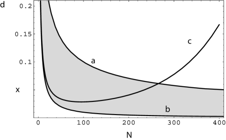
Figure 1: Phase sensitivity $\Delta\phi$ of imperfect noon states with noise parameter $\delta=0.02$ and $\phi=\pi/2N$ as a function of $N$. The shaded area is bounded by the standard quantum limit $1/\sqrt{N}$ and the Heisenberg limit $1/N$. The minimum uncertainty point is given by $N=2/\delta$.

Bootstrapping

If the number of photons in a useful noon states is limited by the phase uncertainty as described above, then these states would be of little use in metrology. However, we can use so-called bootstrapping to increase the effective noon states to arbitrary photon number. The idea behind this technique is to use (noisy) noon states to improve the phase uncertainty in the optical control. For example, suppose that the phase shifters producing the phases in Eq. (2) are implemented with delay lines, and the error $\Delta l$ in the delay is related to $\sqrt{\delta}$ according to $\sqrt{\delta}=k\Delta l$, with $k$ the wave number. The resulting noisy noon state can be used to re-evaluate the length of the delay lines used in the state preparation process. If the error in the length estimation using the noisy noon state is smaller than the initial error $\sqrt{\delta}$, then the delay lines can be set with a higher accuracy. Bootstrapping occurs when this higher accuracy is used to tune smaller increments in the phase shifts and consequently create a larger noisy noon state. This procedure can then be repeated indefinitely.

Clearly, for bootstrapping to work the minimum phase uncertainty $\Delta\varphi_{\rm min}$ obtained by noon states must be smaller than the phase uncertainty $\sqrt{\delta}$ in the apparatus:

$$\Delta\varphi_{\rm min}=\frac{e^{N\delta/2}}{N}<\sqrt{\delta}.$$ (14)

Since the minimum value of the phase uncertainty is reached when $N=2/\delta$, we substitute this into Eq. (14) and solve the inequality. We find that bootstrapping is possible when $\sqrt{\delta}<2/e$. Furthermore, if $\sqrt{\delta_{0}}$ is the initial phase uncertainty and $\sqrt{\delta_{n}}$ is the uncertainty in the $n^{th}$ iteration, the bootstrapping converges to zero super-exponentially:

$$\delta_{n}=\left(\frac{e}{2}\,\delta_{0}\right)^{2^{n}}\quad\text{and}\qquad N_{n}=2\left(\frac{1}{e}\,N_{0}\right)^{2^{n}}.$$ (15)

For an initial phase uncertainty of 0.05 rad, the optimal noon state contains ten photons. After two and three bootstrapping iterations, the optimal noon state contains $\sim 180$ and $10^{5}$ photons, respectively.

Conclusion

I have shown that the limits to optical phase control put a bound on the size of the noon states that can be created with linear optics and projective measurements, while still being able to perform sub-shot-noise phase estimation. If the error in the phase control is given by $\sqrt{\delta}$, then the maximum phase sensitivity in standard Heisenberg-limited metrology is reached when $N=2/\delta$. However, an adaptive bootstrapping technique can be used to create high-fidelity noon states of arbitrary size (high-noon states). Furthermore, this techique reduces the phase uncertainty super-exponentially.

This research is part of the QIP IRC www.qipirc.org (GR/S82176/01), and was inspired by the LOQuIP workshop in Baton Rouge.

References

- Caves (1981) C. M. Caves, Phys. Rev. D 23, 1693 (1981).
- Yurke et al. (1986) B. Yurke, S. L. McCall, and J. Klauder, Phys. Rev. A 33, 4033 (1986).
- Bollinger et al. (1996) J. J. Bollinger, W. M. Itano, D. J. Wineland, and D. J. Heinzen, Phys. Rev. A 54, 4649 (1996).
- Boto et al. (2000) A. N. Boto, P. Kok, D. S. Abrams, S. L. Braunstein, C. P. Williams, and J. P. Dowling, Phys. Rev. Lett. 85, 2733 (2000).
- Kok et al. (2004) P. Kok, S. L. Braunstein, and J. P. Dowling, J. Opt. B 6, S796 (2004).
- Hofmann (2004) H. F. Hofmann, Phys. Rev. A 70, 023812 (2004).
- Combes and Wiseman (2005) J. Combes and H. M. Wiseman, J. Opt. B 7, 14 (2005).
- Pezzé and Smerzi (2005) L. Pezzé and A. Smerzi, arXiv:quant-ph/0508158 (2005).
- Sun et al. (2005) F. W. Sun, Z. Y. Ou, and G. C. Guo, arXiv:quant-ph/0511189 (2005).
- Gerry (2000) C. C. Gerry, Phys. Rev. A 61, 043811 (2000).
- Fiurášek (2002) J. Fiurášek, Phys. Rev. A 65, 053818 (2002).
- Kok et al. (2002) P. Kok, H. Lee, and J. P. Dowling, Phys. Rev. A 65, 052104 (2002).
- Lee et al. (2002) H. Lee, P. Kok, N. J. Cerf, and J. P. Dowling, Phys. Rev. A 65, 030101 (2002).
- Schmidt and Imamolu (1996) H. Schmidt and A. Imamolu, Opt. Lett. 21, 1936 (1996).
- Friedberg et al. (1989) S. H. Friedberg, A. J. Insel, and L. E. Spence, Linear Algebra (Prentice-Hall, 1989).
- Mitchell et al. (2004) M. W. Mitchell, J. S. Lundeen, and A. M. Steinberg, Nature 429, 161 (2004).
- Walther et al. (2004) P. Walther, J.-W. Pan, M. Aspelmeyer, R. Ursinand, S. Gasparoni, and A. Zeilinger, Nature 429, 158 (2004).
- Helstrom (1976) C. W. Helstrom, Quantum Detection and Estimation Theory (Academic Press, 1976).