Quantum random walk of two photons in separable and entangled state

Abstract

We discuss quantum random walk of two photons using linear optical elements. We analyze the quantum random walk using photons in a variety of quantum states including entangled states. We find that for photons initially in separable Fock states, the final state is entangled. For polarization entangled photons produced by type II downconverter, we calculate the joint probability of detecting two photons at a given site. We show the remarkable dependence of the two photon detection probability on the quantum nature of the state. In order to understand the quantum random walk, we present exact analytical results for small number of steps like five. We present in details numerical results for a number of cases and supplement the numerical results with asymptotic analytical results.

I Introduction

A new paradigm in the study of random walks has recently emerged aharonov ; kempe ; sanders ; knight ; zhao ; jeong ; our ; milburn ; lattice ; exp ; bouwmeester ; bose1 ; bose2 ; zubairy ; chaos ; nmr ; ent-knight . The random walker has been assigned an additional quantum degree of freedom which could be spin degree of freedom aharonov . Thus walker goes left or right depending on the spin degree of freedom. The probability of finding the walker at a given site now depends on the spin state of the walker. All this has now been well studied kempe and numerical simulations have been done to find the site distribution after walker has taken large number of steps. Using linear optical elements, Do et al exp have realized the quantum random walk (QRW). However, in their experiments they used a weak coherent field rather than a field with strong quantum character. This is fine if we recall the results of Knight et al knight who showed that QRW of a single walker can be implemented by using classical fields. A similar arrangement is discussed earlier by other authors as well zhao ; jeong . Jeong et al jeong analyzed the cases of a walker in a coherent state and in a single photon state and concluded that the final probability distribution was identical in the two cases; though different from that of the classical random walk (i.e. a walker without the additional quantum degree of freedom). This is explained by Jeong et al jeong in terms of the P-representation of the state of photons. Thus an important question is-what would be a strict QRW which can not be produced by using classical fields. To understand this aspect, we study QRW by two photons in a variety of quantum states including entangled states. We find that even if initially the two photons are in separable Fock states, the final state is entangled. This is quite an interesting quantum property and has no classical counter part. Omar et al bose2 have studied QRW of two nonidentical walkers with entangled initial state and have shown that the final state is entangled depending on the initial entanglement. Our model of QRW is different from that of Ref bose2 as our system can produce entanglement even if initially there is none. This is clearly borne out by our result in Sec.IV A. Further, we calculate photon-photon correlations which in the past have been very successfully used to reveal the quantum character of the fields mandel ; kwiat . We show the remarkable dependence of the two photon detection probability on the quantum nature of the state of photons. We present explicit results for all four Bell states of the incoming photons. Our work thus brings out the role of coherences and entanglement in QRW.

The organization of the paper is as follows. In Sec.II, we present the system of linear optical elements used to realize QRW. In Sec.III, we discuss QRW of a single photon when the photon enters in the arrangement through the two input ports. The state of the incoming photon is a pure state. We present an approximate analysis for the probability of finding the photon at a site after a large number of steps nayak ; brun and compare with the exact numerical results. In Secs.IV and V, we consider QRW of two photons. We derive analytical results for the photon-photon entanglement corresponding to the case when the walkers take only a small number of steps. The analytical results clearly demonstrate the dependence of two photon detection probability on entanglement between the walkers. We evolve a numerical strategy as well as an approximate analysis to obtain results for final state of the photons after a large number of steps. In Sec.IV, we consider the case when the initial state of the photons is separable however the final state of the photons is entangled. Here the entanglement is generated due to the passage of photons through linear optical elements. We also discuss a case when two photons in Fock state are replaced by two photons in coherent states. We point out that QRW in our scheme with photons either in separable Fock states or in an entangled state can not be reproduced by using coherent states. In Sec.V, we discuss QRW of two photons when initial state is an entangled state and discuss the dependence of two photon detection probability on entanglement initially present in the state of the walkers. We present our conclusions in Sec.VI.

II Description of the Arrangement

In Fig. 1, we show a schematic arrangement for realization of QRW on a line using linear optical elements like polarizing beam splitters (PBS) and half wave plates (HWP). The arrangement looks like a large interferometer and has been discussed in an experimental realization of quantum quincunx exp . The photons enter in the arrangement through the two input ports. The state of the photons anywhere along the arrangement can be completely defined in terms of its direction of propagation and state of polarization.

Figure 1: The schematic arrangements for realizing QRW of two entangled walkers. In the inset effect of polarization beam splitter is shown explicitly. The x-polarized photon is transmitted in the same direction but the y-polarized photon is reflected and changed the direction of propagation.

A half wave plate performs Hadamard operation for a single photon in polarization state basis hwp ,

$$|x\rangle\xrightarrow{HWP}\frac{1}{\sqrt{2}}\left(|x\rangle+|y\rangle\right),$$

$$|y\rangle\xrightarrow{HWP}\frac{1}{\sqrt{2}}\left(|x\rangle-|y\rangle\right),$$ (1)

where $|x\rangle$ and $|y\rangle$ are two orthogonal linear polarization states of the photons. The polarizing beam splitter (PBS) produces polarization dependent spatial displacement in the position of the photons. Clearly the displacement will be either in horizontal or in vertical direction depending on the direction of propagation and the state of polarization of the incoming photons. The operation of PBS can be written as

$$\left(\begin{array}[]{c}|h,x\rangle\\ |h,y\rangle\\ |v,x\rangle\\ |v,y\rangle\end{array}\right)\xrightarrow{PBS}\left(\begin{array}[]{cccc}1&0&0&0\\ 0&0&0&1\\ 0&0&1&0\\ 0&1&0&0\end{array}\right)\left(\begin{array}[]{c}|h,x\rangle\\ |h,y\rangle\\ |v,x\rangle\\ |v,y\rangle\end{array}\right),$$ (2)

where $h(v)$ shows the propagation of the photons along the horizontal (vertical) direction. After passing through PBS photons are displaced by one step in the horizontal direction when they come in the state $|h,x\rangle$ or $|v,y\rangle$ and displaced by one step in vertical direction when they come in the state $|h,y\rangle$ or $|v,x\rangle$. Thus, in our scheme, states $|h,x\rangle$, $|h,y\rangle$, $|v,x\rangle$, and $|v,y\rangle$ are corresponding to the states of a four sided coin and the position of the photon along the optical arrangement performs QRW.

The photons enter through the input ports and pass through a half wave plate followed by a PBS. The half wave plate performs Hadamard operation in the polarization space. Then PBS produces shift in the position of the photons depending on the polarization and the direction of the propagation of the incoming photons. Thus each layer of half wave plate followed by the PBS generates one step of QRW in the spatial state of the photons. After particular number of such steps the position of the photons is detected by an array of the detectors. The detection of the photons can be made polarization sensitive or insensitive depending on the particular interest of measurement of the state.

In Fig. 1, we show the arrangement which has five layers, each layer is made of half wave plate followed by a PBS. This arrangement can produce QRW by five steps. Needless to say that for large number of steps a large number of optical elements will be required and such a big arrangement may have some difficulties in alignment as well as the visibility of the signal.

III QRW of a single photon

In this section, we consider the case when a single photon enters through the input ports. Thus we have a single walker and the QRW is controlled by a four sided coin. The four sides of the coin are formed by the four degrees of freedom of the photon, two directions of propagation as the photon can move in horizontal or in the vertical direction, and two directions of polarization. The state of the photon at any time during the QRW can be defined as $|n,q,j,k\rangle$, where $n$ represents the number of steps, $q$ represents the spatial position of the photon with the convention that the horizontal displacement is in $+ve$ direction and the vertical displacement is in $-ve$ direction, and $j$, $k$ represent the direction of propagation and the direction of polarization respectively.

The dynamics of the photon can be described by expressing the state of the photon after $n+1$ steps in terms of the states after $n$ steps in the following way.

$$|n,q,h,x\rangle \xrightarrow{HWP}\frac{1}{\sqrt{2}}(|n,q,h,x\rangle+|n,q,h,y\rangle)$$ (3)

$$\xrightarrow{PBS}\frac{1}{\sqrt{2}}(|n+1,q+1,h,x\rangle+|n+1,q-1,v,y\rangle),$$

$$|n,q,h,y\rangle \xrightarrow{HWP}\frac{1}{\sqrt{2}}(|n,q,h,x\rangle-|n,q,h,y\rangle)$$ (4)

$$\xrightarrow{PBS}\frac{1}{\sqrt{2}}(|n+1,q+1,h,x\rangle-|n+1,q-1,v,y\rangle),$$

$$|n,q,v,x\rangle \xrightarrow{HWP}\frac{1}{\sqrt{2}}(|n,q,v,x\rangle+|n,q,v,y\rangle)$$ (5)

$$\xrightarrow{PBS}\frac{1}{\sqrt{2}}(|n+1,q-1,v,x\rangle+|n+1,q+1,h,y\rangle),$$

$$|n,q,v,y\rangle \xrightarrow{HWP}\frac{1}{\sqrt{2}}(|n,q,v,x\rangle-|n,q,v,y\rangle)$$ (6)

$$\xrightarrow{PBS}\frac{1}{\sqrt{2}}(|n+1,q-1,v,x\rangle-|n+1,q+1,h,y\rangle).$$

First the half wave plate generates transformation in the polarization states of the photon which is followed by the spatial transformation generated by the PBS. We can reexpress Eqs. (3)-(6) in terms of operators $C$ and $S$, equivalently, as

$$\left[\begin{array}[]{c}|n+1,q+1,h,x\rangle\\ |n+1,q+1,h,y\rangle\\ |n+1,q-1,v,x\rangle\\ |n+1,q-1,v,y\rangle\end{array}\right]\equiv S\otimes C\left[\begin{array}[]{c}|n,q,h,x\rangle\\ |n,q,h,y\rangle\\ |n,q,v,x\rangle\\ |n,q,v,y\rangle\end{array}\right],$$ (7)

where $C$ and $S$ are

$$C=\frac{1}{\sqrt{2}}\left(|h,x\rangle\langle h,x|+|h,x\rangle\langle h,y|+|h,y\rangle\langle v,x|-|h,y\rangle\langle v,y|\right.$$

$$\left.+|v,x\rangle\langle v,x|+|v,x\rangle\langle v,y|+|v,y\rangle\langle h,x|-|v,y\rangle\langle h,y|\right)~{}$$ (8)

$$S\equiv|h,x\rangle\langle h,x|\otimes|q+1\rangle\langle q|+|h,y\rangle\langle h,y|\otimes|q+1\rangle\langle q|$$

$$+|v,x\rangle\langle v,x|\otimes|q-1\rangle\langle q|+|v,y\rangle\langle v,y|\otimes|q-1\rangle\langle q|$$ (9)

Thus, the unitary coin operator $C$ and the conditioned shift operator $S$ for the QRW of the photon are given by Eqs. (8) and (9) respectively. The transformation $U_{s}\equiv S\otimes C$ acting on the initial state of the photon is equivalent to the one step of QRW. The iterative application of the transformation $U_{s}$ for $n$ times, $U_{s}^{n}$, gives the QRW of $n$ steps.

Figure 2: (Color online) The probability distribution $P(q)$ for detecting the walker at position $q$, for the initial coin state (a) $\frac{1}{\sqrt{2}}(|h,x\rangle+|v,y\rangle)$ and (b)$\frac{1}{\sqrt{2}}(|h,x\rangle-|v,y\rangle)$. The black solid (red dashed) line is corresponding to exact (approximated) values.

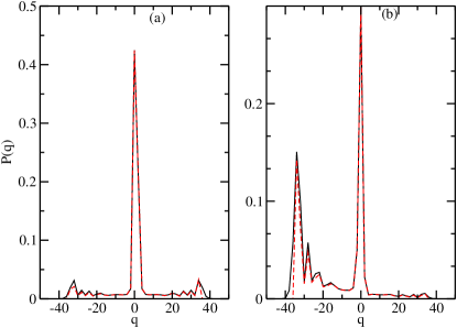
Figure 3: (Color online) The probability distribution $P(q)$ for detecting the walker at position $q$, for the initial coin state (a) $\frac{1}{\sqrt{2}}(|h,y\rangle+|v,x\rangle)$ and (b)$\frac{1}{\sqrt{2}}(|h,y\rangle-|v,x\rangle)$. The black solid (red dashed) line is corresponding to exact (approximated) values.

The initial state of the coin can be selected as one of the states, $|h,x\rangle$, $|h,y\rangle$, $|v,x\rangle$, $|v,y\rangle$, and their possible superpositions. For a classical analog to this QRW we look at the shift operator $S$ defined by Eq.(9). Clearly, this walk is equivalent to the random walk of a single walker with four dimensional coin where walker moves one step forward for two possible outcomes of the coin and moves one step backward for the other two. The probability of reaching the walker at position $q$ will be a binomial distribution

$$P(q)=\frac{n!}{\frac{n+q}{2}!\frac{n-q}{2}!}\frac{1}{2^{n}}.$$ (10)

Thus classically we can not differentiate between the walk of single photon in this case and the walk of a single walker with two sided coin. In the following we show how QRW of single photon in this case leads to different results than QRW with a two sided coin.

Here we present an approximate analysis of QRW for large number of steps. We follow a similar method as discussed by Nayak et al nayak and Brun et al brun using discrete spatial Fourier transform and taking asymptotic limit of the Fourier integrals for large number of steps. We relegate the details to the appendix. For initial coin state $|h,x\rangle$, we get the final state of the photon $|\Psi_{hx}(n)\rangle$ after $n$ steps as follows.

$$|\Psi_{hx}(n)\rangle=\sum_{q=-n}^{n}|\psi_{hx}(n,q)\rangle,$$ (11)

$$|\psi_{hx}(n,q)\rangle=f_{hx}|n,q,h,x\rangle+f_{hy}|n,q,h,y\rangle+f_{vx}|n,q,v,x\rangle+f_{vy}|n,q,v,y\rangle,$$ (12)

where the coefficients $f_{\mu\nu}$ are given by

$$f_{hx}=\frac{1+(-1)^{n+q}}{8\pi}\left[\int_{-\pi}^{\pi}\frac{\cos(kq)}{2-\sqrt{2}\cos k}dk+\sqrt{\frac{2\pi}{n|\phi^{\prime\prime}(k_{0})|}}\frac{3C(n,q)-\sqrt{2}C(n-1,q+1)-\sqrt{2}C(n+1,q-1)}{1+\sin^{2}k_{0}}\right],$$ (13)

$$f_{hy}=\frac{1+(-1)^{n+q}}{8\pi}\left[\int_{-\pi}^{\pi}\frac{\sqrt{2}\cos[k(q+1)]-\cos(kq)}{2-\sqrt{2}\cos k}dk+\sqrt{\frac{2\pi}{n|\phi^{\prime\prime}(k_{0})|}}\frac{C(n,q)-\sqrt{2}C(n-1,q+1)}{1+\sin^{2}k_{0}}\right],$$ (14)

$$f_{vx}=\frac{1+(-1)^{n+q}}{8\pi}\left[\int_{-\pi}^{\pi}\frac{\cos[k(q+2)]}{2-\sqrt{2}\cos k}dk-\sqrt{\frac{2\pi}{n|\phi^{\prime\prime}(k_{0})|}}\frac{C(n,q+2)}{1+\sin^{2}k_{0}}\right],$$ (15)

$$f_{vy}=\frac{1+(-1)^{n+q}}{8\pi}\left[\int_{-\pi}^{\pi}\frac{\sqrt{2}\cos[k(q+1)]-\cos[k(q+2)]}{2-\sqrt{2}\cos k}dk+\sqrt{\frac{2\pi}{n|\phi^{\prime\prime}(k_{0})|}}\frac{\sqrt{2}C(n-1,q+1)-C(n,q)}{1+\sin^{2}k_{0}}\right],$$ (16)

$$C(n,q)=\cos(n\omega_{0}+qk_{0}+\pi/4),~{}~{}\omega_{0}=\omega_{k}|_{k=k_{0}},$$ (17)

where $\phi(k)=-(\omega_{k}+k\alpha)$, $\alpha=q/n$, $\omega_{k}\in[\pi/4,3\pi/4]$ and defined as $\cos\omega_{k}=\cos k/\sqrt{2}$, $k_{0}=\sin^{-1}(-\alpha/\sqrt{1-\alpha^{2}})$ and prime denotes the derivative with respect to $k$. This approximation is valid in the interval $\alpha\in[-1/\sqrt{2},1/\sqrt{2}]$, outside of this interval $f_{\mu\nu}$ can be taken zero. In the expressions of $f_{\mu\nu}$, the integral inside the bracket is independent of $n$, and is responsible for the constant spikes in the probability of detecting photon near initial position $q=0$. We evaluate this integral numerically. The second term inside the bracket is sum of cosines and completely characterizes QRW. Similarly, for initial coin state $|h,y\rangle$, the state of the photon after $n$ steps is

$$|\Psi_{hy}(n)\rangle=\sum_{q=-n}^{n}|\psi_{hy}(n,q)\rangle,$$ (18)

$$|\psi_{hy}(n,q)\rangle=g_{hx}|n,q,h,x\rangle+g_{hy}|n,q,h,y\rangle+g_{vx}|n,q,v,x\rangle+g_{vy}|n,q,v,y\rangle,$$ (19)

where

$$g_{hx}=\frac{1+(-1)^{n+q}}{8\pi}\left[\int_{-\pi}^{\pi}\frac{\sqrt{2}\cos[k(q-1)]-\cos(kq)}{2-\sqrt{2}\cos k}dk+\sqrt{\frac{2\pi}{n|\phi^{\prime\prime}(k_{0})|}}\frac{C(n,q)-\sqrt{2}C(n+1,q-1)}{1+\sin^{2}k_{0}}\right],$$ (20)

$$g_{hy}=\frac{1+(-1)^{n+q}}{8\pi}\left[\int_{-\pi}^{\pi}\frac{(3-2\sqrt{2}\cos k)\cos(kq)}{2-\sqrt{2}\cos k}dk+\sqrt{\frac{2\pi}{n|\phi^{\prime\prime}(k_{0})|}}\frac{C(n,q)}{1+\sin^{2}k_{0}}\right],$$ (21)

$$g_{vx}=\frac{1+(-1)^{n+q}}{8\pi}\left[\int_{-\pi}^{\pi}\frac{\sqrt{2}\cos[k(q+1)]-\cos[k(q+2)]}{2-\sqrt{2}\cos k}dk+\sqrt{\frac{2\pi}{n|\phi^{\prime\prime}(k_{0})|}}\frac{\sqrt{2}C(n+1,q+1)-C(n,q)}{1+\sin^{2}k_{0}}\right],$$ (22)

$$g_{vy}=\frac{1+(-1)^{n+q}}{8\pi}\left[\int_{-\pi}^{\pi}\frac{2\cos kq-2\sqrt{2}\cos[k(q+1)]+\cos[k(q+2)]}{2-\sqrt{2}\cos k}dk-\sqrt{\frac{2\pi}{n|\phi^{\prime\prime}(k_{0})|}}\frac{C(n,q)}{1+\sin^{2}k_{0}}\right].$$ (23)

From the symmetry of the arrangement (see Fig. 1), the state of the photon after $n$ steps for initial coin states $|v,x\rangle$ and $|v,y\rangle$ can be written by interchanging the direction of propagation $h$ and $v$ and replacing $q$ by $-q$ in $|\Psi_{hx}(n)\rangle$ and $|\Psi_{hy}(n)\rangle$ respectively.

$$|\Psi_{vx}(n)\rangle=\sum_{q=-n}^{n}|\psi_{vx}(n,q)\rangle,$$ (24)

$$|\Psi_{vy}(n)\rangle=\sum_{q=-n}^{n}|\psi_{vy}(n,q)\rangle,$$ (25)

$$|\psi_{vx}(n,-q)\rangle=f_{hx}|n,-q,v,x\rangle+f_{hy}|n,-q,v,y\rangle+f_{vx}|n,-q,h,x\rangle+f_{vy}|n,-q,h,y\rangle,$$ (26)

$$|\psi_{vy}(n,-q)\rangle=g_{hx}|n,-q,v,x\rangle+g_{hy}|n,-q,v,y\rangle+g_{vx}|n,-q,h,x\rangle+g_{vy}|n,-q,h,y\rangle.$$ (27)

For initial coin state as an arbitrary superposition $\alpha|h,x\rangle+\beta|v,y\rangle$, the state of the photon after $n$ steps is given by

$$|\Psi(n)\rangle=\alpha|\Psi_{hx}(n)\rangle+\beta|\Psi_{vy}(n)\rangle.$$ (28)

In Figs. 2 and 3, we have shown the probability distribution for QRW of the single photon with initial coin states $\frac{1}{\sqrt{2}}(|h,x\rangle\pm|v,y\rangle)$ and $\frac{1}{\sqrt{2}}(|h,y\rangle\pm|v,x\rangle)$ after $50$ steps. We plot the results using above approximate analysis as well as exact numerical simulations. Clearly for large number of steps, say for $n=50$, there are very small differences between the approximate analysis and the exact simulations. Further for larger values of $n$ these differences will be negligible. It should be noted that the probability distributions for detecting the photon at position $q$ in Figs. 2 and 3 are very much different than the distributions for QRW with a two sided coin kempe . In all these cases the initial state is most probable state and the distribution is sharply peaked at $q=0$. For initial coin states $\frac{1}{\sqrt{2}}(|h,x\rangle+|v,y\rangle)$ and $\frac{1}{\sqrt{2}}(|h,y\rangle+|v,x\rangle)$ the distributions are symmetric but the side peaks are very small and most of the time walker remains at its initial position very precisely. In the case of QRW with initial coin states $\frac{1}{\sqrt{2}}(|h,x\rangle-|v,y\rangle)$ and $\frac{1}{\sqrt{2}}(|h,y\rangle-|v,x\rangle)$, in addition to the narrow central peak, distributions have a peak along one side of the position axis. Further for the state $\frac{1}{\sqrt{2}}(|h,x\rangle-|v,y\rangle)$ the additional peak in the distribution is along the positive side of the axis at $q=n/\sqrt{2}$, while for state $\frac{1}{\sqrt{2}}(|h,y\rangle-|v,x\rangle)$ the additional peak is along the negative side at $q=-n/\sqrt{2}$. We emphasize that the quantum random walk of a single photon depends very much on the initial state, see for example the distinction between the Figs. 2(a) and 2(b).

IV QRW of Two photons with separable initial state

In recent papers knight , it has been shown that QRW is an interference phenomenon and does not essentially depend on the quantum nature of the state of the walker. As a result various classical sources like low intensity lasers exp ; bouwmeester and coherent state of radiation fields milburn ; our are used to realize QRW. In order to explore further the quantum nature of random walk, we consider the case when two photons start QRW from a separable initial state

$$|\Psi\rangle=|\Psi_{1}\rangle\otimes|\Psi_{2}\rangle,$$ (29)

where $|\Psi\rangle$ is state of two photons and $|\Psi_{1}\rangle$ and $|\Psi_{2}\rangle$ are states of single photons. The state of the photons after a certain number of steps is, in general, not a separable state as quantum entanglement is produced by linear optical elements. This is reminiscent of the well known property mandel of a 50-50 beam splitter where two incoming photons in the separable state $|1,1\rangle$ go over to an entangled state of the form $(|2,0\rangle+|0,2\rangle)/\sqrt{2}$. We first consider the case of input states which are single photon states. We would also consider the case when the input states are replaced by coherent states

IV.1 QRW of two photons with initially in separable Fock states

In our scheme, two photons act as two walkers. They enter in the arrangement through the two input ports. Initially one photon propagates in horizontal direction and the other in vertical direction. We consider the initial state of the photons as one of the four separable states $|0,0,h,x\rangle\otimes|0,0,v,x\rangle$, $|0,0,h,y\rangle\otimes|0,0,v,y\rangle$, $|0,0,h,x\rangle\otimes|0,0,v,y\rangle$, and $|0,0,h,y\rangle\otimes|0,0,v,x\rangle$. We can write these states in terms of initial field operators as follow.

$$|0,0,h,x\rangle\otimes|0,0,v,x\rangle\equiv a^{(0,0){\dagger}}_{hx}a^{(0,0){\dagger}}_{vx}|0\rangle,$$ (30)

$$|0,0,h,x\rangle\otimes|0,0,v,y\rangle\equiv a^{(0,0){\dagger}}_{hx}a^{(0,0){\dagger}}_{vy}|0\rangle,$$ (31)

$$|0,0,h,y\rangle\otimes|0,0,v,y\rangle\equiv a^{(0,0){\dagger}}_{hy}a^{(0,0){\dagger}}_{vy}|0\rangle,$$ (32)

$$|0,0,h,y\rangle\otimes|0,0,v,x\rangle\equiv a^{(0,0){\dagger}}_{hy}a^{(0,0){\dagger}}_{vx}|0\rangle,$$ (33)

where $a^{(n,q){\dagger}}_{jk}$ is creation operator for a photon, $a^{(n,q){\dagger}}_{jk}|0\rangle\equiv|n,q,j,k\rangle$, and $|0\rangle$ is vacuum. Here we present the analytical calculations for QRW of few steps, say five steps. For linear optical elements, it is sometimes instructive and transparent to work with the transformation of operators. This is particularly so if the states with more than one photons are involved. Thus for calculating final state of the walkers after five steps, we express the initial field operators, $a_{jk}^{(0,0)}$, in terms of the final field operators, $a^{(5,q)}_{jk}$, after five steps.

$$a_{hx}^{(0,0)} = \frac{1}{4\sqrt{2}}(a^{(5,-5)}_{vx}+a^{(5,-3)}_{hy}+a^{(5,-3)}_{vx}-a^{(5,-3)}_{vy}+a^{(5,-1)}_{hx}$$ (34)

$$+ 3a^{(5,-1)}_{hy}+a^{(5,-1)}_{vx}+a^{(5,-1)}_{vy}+a^{(5,1)}_{hx}+a^{(5,1)}_{hy}+a^{(5,1)}_{vx}$$

$$- a^{(5,1)}_{vy}-3a^{(5,3)}_{hx}-a^{(5,3)}_{hy}+a^{(5,3)}_{vy}+a^{(5,5)}_{hx}),$$

$$a_{hy}^{(0,0)} = \frac{1}{4\sqrt{2}}(-a^{(5,-5)}_{vx}-a^{(5,-3)}_{hy}+a^{(5,-3)}_{vx}+a^{(5,-3)}_{vy}-a^{(5,-1)}_{hx}$$ (35)

$$- a^{(5,-1)}_{hy}+3a^{(5,-1)}_{vx}-3a^{(5,-1)}_{vy}+a^{(5,1)}_{hx}-a^{(5,1)}_{hy}+a^{(5,1)}_{vx}$$

$$+ a^{(5,1)}_{vy}-a^{(5,3)}_{hx}-a^{(5,3)}_{hy}+a^{(5,3)}_{vy}+a^{(5,5)}_{hx}),$$

$$a_{vx}^{(0,0)} = \frac{1}{4\sqrt{2}}(a^{(5,-5)}_{vx}+a^{(5,-3)}_{hy}-3a^{(5,-3)}_{vx}-a^{(5,-3)}_{vy}+a^{(5,-1)}_{hx}$$ (36)

$$- a^{(5,-1)}_{hy}+a^{(5,-1)}_{vx}+a^{(5,-1)}_{vy}+a^{(5,1)}_{hx}+a^{(5,1)}_{hy}+a^{(5,1)}_{vx}$$

$$+ 3a^{(5,1)}_{vy}+a^{(5,3)}_{hx}-a^{(5,3)}_{hy}+a^{(5,3)}_{vy}+a^{(5,5)}_{hx}),$$

$$a_{vy}^{(0,0)} = \frac{1}{4\sqrt{2}}(a^{(5,-5)}_{vx}+a^{(5,-3)}_{hy}-a^{(5,-3)}_{vx}-a^{(5,-3)}_{vy}+a^{(5,-1)}_{hx}$$ (37)

$$+ a^{(5,-1)}_{hy}+a^{(5,-1)}_{vx}-a^{(5,-1)}_{vy}+3a^{(5,1)}_{hx}-3a^{(5,1)}_{hy}-a^{(5,1)}_{vx}$$

$$- a^{(5,1)}_{vy}+a^{(5,3)}_{hx}+a^{(5,3)}_{hy}-a^{(5,3)}_{vy}-a^{(5,5)}_{hx}).$$

Using transformations (34) to (37) and Eqs. (30) to (33), the state of the quantum walkers, corresponding to a particular initial state, after five steps can be calculated. Clearly, the final state of the photons is an entangled state and can not be expressed as a product of the states of two single photons.

$$|\bar{\Psi}\rangle\neq|\bar{\Psi}_{1}\rangle\otimes|\bar{\Psi}_{2}\rangle,$$ (38)

where $|\bar{\Psi}\rangle$ is final state of two photons and $|\bar{\Psi}_{1}\rangle$ and $|\bar{\Psi}_{2}\rangle$ are final states of single photons. It should be borne in mind that Eqs.(34) to (37) should be supplemented by free field operators at the open ports. These are important for the operator algebra. However these do not contribute to the results below and hence for brevity we have not written these explicitly in Eqs.(34) - (37).

Finally, the results for calculated probability $P(q_{1},q_{2})$ for detecting the walkers at positions $q_{1}$ and $q_{2}$ simultaneously, after five steps, are shown in the Table.I. Note that the diagonal elements $P(q,q)$ give the probability of finding two photons at the site $q$. It is clear from the Table.I that the probability distributions for all considered initial states are different to each other. At the bottom of the table we present the probability $P(q_{1})$ of detecting at least one photon at the position $q_{1}$, where $P(q_{1})=\sum_{q_{2}}P(q_{1},q_{2})$. Further using the values of $P(q_{1},q_{2})$ and $P(q_{1})$, $P(q_{2})$ for the positions $q_{1}$ and $q_{2}$ we can also calculate the correlation

$$\sigma_{q_{1}q_{2}}=P(q_{1},q_{2})-P(q_{1})P(q_{2}).$$ (39)

We found that the correlation $\sigma_{q_{1}q_{2}}$ is non zero almost everywhere for all values of $P(q_{1},q_{2})$, which shows that though initially walkers were in a separable state, but after few steps their state is entangled. We emphasize that the correlation (39) is due to quantum as the state (38) does not factorize. These correlations are due to the quantum nature of the initial state and arise when the photons pass through the linear optical elements. The origin of such correlations has been observed by Mandel and coworkers mandel in their pioneer work on beam splitters. It should be noted here that if we replace the photons with two coherent states the output state will be a factorized state and the probability distribution will not exhibit such correlations. Thus the QRW of two photons is completely dependent of quantum nature of the state of the photons and no coherent state can reproduce such QRW. It should be noted that the normalization condition for $P(q_{1},q_{2})$ is given by $\sum_{q_{1}\geq q_{2}}P(q_{1},q_{2})=1$. Further $\sum_{q_{1}}P(q_{1})$ is not equal to $1$ and the normalization condition for $P(q_{1})$ will be $\sum_{q_{1}}P(q_{1})+P(q_{1},q_{1})=2$. To see it more clearly consider the following state of finding two photons at sites $1$ and $2$,

$$|\psi\rangle=\frac{1}{\sqrt{3}}\left(|1,1\rangle+|1,2\rangle+|2,2\rangle\right)$$ (40)

For this state the probabilities of detecting at least one photon at site $1$ and $2$ are $P(1)=P(2)=2/3$ and the probabilities of detecting both photons at same site are $P(1,1)=P(2,2)=1/3$ which satisfy the above normalization condition.

Table 1: The calculated probabilities of detection for the photons after five steps, for initial state (a) $|0,0,h,x\rangle\otimes|0,0,v,x\rangle$, (b) $|0,0,h,x\rangle\otimes|0,0,v,y\rangle$, (c) $|0,0,h,y\rangle\otimes|0,0,v,y\rangle$, and (d) $|0,0,h,y\rangle\otimes|0,0,v,x\rangle$. All values shown in the table are $128$ times of the actual values.

(a) $P(q_{1},q_{2})$ $q_{1}=-5$ $q_{1}=-3$ $q_{1}=-1$ $q_{1}=1$ $q_{1}=3$ $q_{1}=5$ $q_{2}=-5$ 0.25 1.5 2 2 1.5 0.5 $q_{2}=-3$ 1.5 4.25 18 10 16.5 1.5 $q_{2}=-1$ 2 18 6 20 10 2 $q_{2}=1$ 2 10 20 6 18 2 $q_{2}=3$ 1.5 16.5 10 18 4.25 1.5 $q_{2}=5$ 0.5 1.5 2 2 1.5 0.25 $P(q_{1})$ 7.75 51.75 58 58 51.75 7.75	(b) $P(q_{1},q_{2})$ $q_{1}=-5$ $q_{1}=-3$ $q_{1}=-1$ $q_{1}=1$ $q_{1}=3$ $q_{1}=5$ $q_{2}=-5$ 0.25 1 3 3 0.5 0 $q_{2}=-3$ 1 1.25 7 9 4 0.5 $q_{2}=-1$ 3 7 8 32 5 1 $q_{2}=1$ 3 9 32 10 29 3 $q_{2}=3$ 0.5 4 5 29 7.25 3 $q_{2}=5$ 0 0.5 1 3 3 0.25 $P(q_{1})$ 7.75 22.75 56 86 48.75 7.75
(c) $P(q_{1},q_{2})$ $q_{1}=-5$ $q_{1}=-3$ $q_{1}=-1$ $q_{1}=1$ $q_{1}=3$ $q_{1}=5$ $q_{2}=-5$ 0.25 1.5 2 2 1.5 0.5 $q_{2}=-3$ 1.5 2.25 6 6 4.5 1.5 $q_{2}=-1$ 2 6 12 56 6 2 $q_{2}=1$ 2 6 56 12 6 2 $q_{2}=3$ 1.5 4.5 6 6 2.25 1.5 $q_{2}=5$ 0.5 1.5 2 2 1.5 0.25 $P(q_{1})$ 7.75 21.75 84 84 21.75 7.75	(d) $P(q_{1},q_{2})$ $q_{1}=-5$ $q_{1}=-3$ $q_{1}=-1$ $q_{1}=1$ $q_{1}=3$ $q_{1}=5$ $q_{2}=-5$ 0.25 3 3 1 0.5 0 $q_{2}=-3$ 3 7.25 29 5 4 0.5 $q_{2}=-1$ 3 29 10 32 9 3 $q_{2}=1$ 1 5 32 8 7 3 $q_{2}=3$ 0.5 4 9 7 1.25 1 $q_{2}=5$ 0 0.5 3 3 1 0.25 $P(q_{1})$ 7.75 48.75 86 56 22.75 7.75

Figure 4: (Color online) The probability $P(q_{1},q_{2})$ of detecting the walkers at positions $q_{1}$ and $q_{2}$ after number of steps $n=25$. The walkers come in the separable state (a) $|0,0,h,x\rangle\otimes|0,0,v,x\rangle$, (b) $|0,0,h,x\rangle\otimes|0,0,v,y\rangle$, (c) $|0,0,h,y\rangle\otimes|0,0,v,y\rangle$, and (d) $|0,0,h,y\rangle\otimes|0,0,v,x\rangle$.

After providing an approach to the analytical calculations for few steps, we present numerical simulations for larger number of steps. The operator $U=(S\otimes C)\otimes(S\otimes C)$ acting on the initial state of the photons generates QRW of one step. Thus the transformation $U^{n}$ will give the final state of the random walkers after $n$ steps. Here unitary coin operator $C$ and the conditioned shift operator $S$ for QRW are given by the Eqs. (8) and (9) of the previous section.

In Fig. 4 we have plotted the probability distributions for detecting photons at positions $q_{1}$ and $q_{2}$ simultaneously after $25$ steps of QRW. In Fig. 4 the photons are in separable initial states. We notice that each probability distribution is very much different from the other. A very common feature in all plots is sharp central peak which shows that in all cases the initial state is the most probable state. In fact this is the property of classical random walk, which has Gaussian probability distribution, but in Fig. 4 the central peak is much narrower than a Gaussian distribution and the large spread of the distribution has strickenly different behavior.

For approximate analytical calculations for large number of steps we use the results (12), (19), (26) and (27) in the following way. For example, for initial state $|0,0,h,x\rangle\otimes|0,0,v,y\rangle$, the state of the photons after $n$ steps will be

$$|\Psi_{xy}(n)\rangle=\frac{1}{\sqrt{2}}\sum_{q_{1},q_{2}=-n}^{n}\left[|\psi_{hx}(n,q_{1})\rangle\otimes|\psi_{vy}(n,q_{2})\rangle+|\psi_{hx}(n,q_{2})\rangle\otimes|\psi_{vy}(n,q_{1})\rangle\right].$$ (41)

Here $|\Psi_{xy}(n)\rangle$ has exchange degeneracy as both photons are undistinguished after they have passed through the optical arrangement. Similarly, we can calculate the final state of the photons for other separable initial states shown in Fig.4. We have checked that the joint probability distributions $P(q_{1},q_{2})$ for large number of steps calculated using above approximate analysis match with the exact simulations. Thus our approximate analysis can be used to calculate the correlations between the walkers after large number of steps very well.

Here we have explicitly shown that in our case QRW of two photons is highly entangled, even though the photons start in separable states. The entanglement is developed in the course of time when the photons pass through the optical arrangement. In the next subsection we show that the QRW of two photons in our case can not be produced by using coherent states.

IV.2 QRW of two photons initially in separable coherent states

Here we discuss the case of QRW when two photons in our scheme are replaced with two weak coherent states. Let us consider that the initial state is

$$|\psi(0)\rangle=|\alpha\rangle_{hx}^{(0,0)}|\beta\rangle_{vy}^{(0,0)},$$ (42)

where indices to the coherent states $|\alpha\rangle$ and $|\beta\rangle$ have their earlier assigned meanings. The initial state in terms of field operators can be expressed as coherent

$$|\psi(0)\rangle=\exp(\alpha a^{(0,0){\dagger}}_{hx}-\alpha^{*}a_{hx}^{(0,0)})\exp(\beta a^{(0,0){\dagger}}_{vy}-\beta^{*}a_{vy}^{(0,0)})|0\rangle.$$ (43)

Now using transformations (34), (37) and Eq.(43) the final state, after five steps of QRW, is given by

$$|\psi(5)\rangle=|\frac{\alpha+\beta}{4\sqrt{2}}\rangle^{(5,-5)}_{vx}|\frac{\alpha+\beta}{4\sqrt{2}}\rangle^{(5,-3)}_{hy}|\frac{\alpha-\beta}{4\sqrt{2}}\rangle^{(5,-3)}_{vx}|\frac{-\alpha-\beta}{4\sqrt{2}}\rangle^{(5,-3)}_{vy}$$

$$\otimes|\frac{\alpha+\beta}{4\sqrt{2}}\rangle^{(5,-1)}_{hx}|\frac{3\alpha+\beta}{4\sqrt{2}}\rangle^{(5,-1)}_{hy}|\frac{\alpha+\beta}{4\sqrt{2}}\rangle^{(5,-1)}_{vx}|\frac{\alpha-\beta}{4\sqrt{2}}\rangle^{(5,-1)}_{vy}$$

$$\otimes|\frac{\alpha+3\beta}{4\sqrt{2}}\rangle^{(5,1)}_{hx}|\frac{\alpha-3\beta}{4\sqrt{2}}\rangle^{(5,1)}_{hy}|\frac{\alpha-\beta}{4\sqrt{2}}\rangle^{(5,1)}_{vx}|\frac{-\alpha-\beta}{4\sqrt{2}}\rangle^{(5,1)}_{vy}$$

$$\otimes|\frac{-3\alpha+\beta}{4\sqrt{2}}\rangle^{(5,3)}_{hx}|\frac{-\alpha+\beta}{4\sqrt{2}}\rangle^{(5,3)}_{hy}|\frac{\alpha-\beta}{4\sqrt{2}}\rangle^{(5,3)}_{vy}|\frac{\alpha-\beta}{4\sqrt{2}}\rangle^{(5,5)}_{hx},~{}~{}$$ (44)

where superscript $(5,q)$ on each state in (44) denotes the position of the photons at $q$ after $5$ steps. Clearly the final state (44) is a product state and the value of correlation $\sigma_{q_{1}q_{2}}$ defined by (39) will be zero for such state.

Note that the probability of finding one photon in a coherent state $|\alpha\rangle$ is $|\alpha|^{2}e^{-|\alpha|^{2}}$. For small enough $|\alpha|$, it reduces to $|\alpha|^{2}$ which is the mean number of photons in a coherent state. Thus, the normalized probability $P(q)$ of detecting a photon at $q$ in this case is equal to the average number of photons detected at site $q$ divided by the average number of incident photons $|\alpha|^{2}+|\beta|^{2}$.

In Table.II, we show the normalized probabilities of detecting photon at site $q$ for small values of $\alpha$ and $\beta$. By comparison of the cases corresponding to $\alpha=f$, $\beta=f$ and $\alpha=f$, $\beta=0$, where $|f|\ll 1$, we see how the interference effects change these probabilities. Similarly for $\alpha=f$, $\beta=f$ and $\alpha=0$, $\beta=f$, the probabilities depend on the interference among various paths. Further these probabilities for one photon detection are different from those listed in the Table. I(b), for the case of two photons in separable Fock states $|0,0,h,x\rangle\otimes|0,0,v,y\rangle$.

Table 2: The normalized probability $P(q)$ of detecting single photon at particular position $q$, after QRW of $5$ steps with initial state $|\alpha\rangle_{hx}^{(0,0)}|\beta\rangle_{vy}^{(0,0)}$, for small amplitudes $\alpha$ and $\beta$.

Probability $P(q)$
$\alpha$	$\beta$	$q=-5$	$q=-3$	$q=-1$	$q=1$	$q=3$	$q=5$
$f$	$f$	1/16	1/8	3/8	3/8	1/16	0
$f$	$-f$	0	1/16	1/8	3/8	3/8	1/16
$f$	$0$	1/32	3/32	3/8	1/8	11/32	1/32
$0$	$f$	1/32	3/32	1/8	5/8	3/32	1/32

It is noted that the normalized probability distribution of detecting photons at particular position $q$ for such initial states is identical to the case of single walker discussed in Sec.III, not to the case of two walkers in Sec.IV A. For example, for $\alpha=f$ and $\beta=f$ the distribution is identical to Fig.2(a) and for $\alpha=f$, $\beta=-f$ we get distribution identical to Fig.2(b). This can be explained by examining the projection of state (42) in one photon space, $|\psi_{0}\rangle\rightarrow\alpha|h,x\rangle\otimes|0\rangle+\beta|0\rangle\otimes|v,y\rangle$ as the contributions from spaces containing more than one photon are of higher order in $\alpha$ and $\beta$.

V QRW of Two photons in entangled state

Here we consider the case when photons start QRW in an entangled state. Thus one photon enters from each input port and the state of the photons is maximally entangled in polarization basis, as those produced by a type-II downconverter. We consider that the state of the photons at input ports is one of the four Bell’s states bell ,

$$|\psi^{\pm}\rangle=\frac{1}{\sqrt{2}}(|0,0,h,x\rangle\otimes|0,0,v,y\rangle\pm|0,0,h,y\rangle\otimes|0,0,v,x\rangle),$$ (45)

$$|\phi^{\pm}\rangle=\frac{1}{\sqrt{2}}(|0,0,h,x\rangle\otimes|0,0,v,x\rangle\pm|0,0,h,y\rangle\otimes|0,0,v,y\rangle).$$ (46)

The states (45) and (46) can be written, in terms of the field operators, as

$$|\psi^{\pm}\rangle=\frac{1}{\sqrt{2}}(a^{(0,0){\dagger}}_{hx}a^{(0,0){\dagger}}_{vy}\pm a^{(0,0){\dagger}}_{hy}a^{(0,0){\dagger}}_{vx})|0\rangle,$$ (47)

$$|\phi^{\pm}\rangle=\frac{1}{\sqrt{2}}(a^{(0,0){\dagger}}_{hx}a^{(0,0){\dagger}}_{vx}\pm a^{(0,0){\dagger}}_{hy}a^{(0,0){\dagger}}_{vy})|0\rangle,$$ (48)

Following a similar procedure as discussed in Sec.IV, we can calculate the final state of photons after five steps using transformations (34) to (37) and Eqs. (47) to (48). In this case also we find that the final state of the photons is an entangled state. Thus in this case both initial and final states of the walkers are entangled state and no classical analog for such states is possible.

In Table. III, we show the results for detecting the photons simultaneously when they start QRW from one of the Bell’s states (47) and (48). We notice that the differences between the distributions for symmetric states and antisymmetric states are much larger than the differences between the distributions for symmetric-symmetric or antisymmetric-antisymmetric states. In terms of correlation (39), both the initial and the final states are highly correlated.

Table 3: The calculated probabilities of detection for the photons after five steps, for initial state (a) $1/\sqrt{2}\left(|0,0,h,x\rangle\otimes|0,0,v,y\rangle+|0,0,h,y\rangle\otimes|0,0,v,x\rangle\right)$, (b) $1/\sqrt{2}\left(|0,0,h,x\rangle\otimes|0,0,v,y\rangle-|0,0,h,y\rangle\otimes|0,0,v,x\rangle\right)$, (c) $1/\sqrt{2}\left(|0,0,h,x\rangle\otimes|0,0,v,x\rangle+|0,0,h,y\rangle\otimes|0,0,v,y\rangle\right)$, and (d) $1/\sqrt{2}\left(|0,0,h,x\rangle\otimes|0,0,v,x\rangle-|0,0,h,y\rangle\otimes|0,0,v,y\rangle\right)$. All values shown in the table are $128$ times of the actual values.

(a) $P(q_{1},q_{2})$ $q_{1}=-5$ $q_{1}=-3$ $q_{1}=-1$ $q_{1}=1$ $q_{1}=3$ $q_{1}=5$ $q_{2}=-5$ 0 1 3 3 1 0 $q_{2}=-3$ 1 4 15 7 8 1 $q_{2}=-1$ 3 15 9 34 7 3 $q_{2}=1$ 3 7 34 9 15 3 $q_{2}=3$ 1 8 7 15 4 1 $q_{2}=5$ 0 1 3 3 1 0 $P(q_{1})$ 8 36 71 71 36 8	(b) $P(q_{1},q_{2})$ $q_{1}=-5$ $q_{1}=-3$ $q_{1}=-1$ $q_{1}=1$ $q_{1}=3$ $q_{1}=5$ $q_{2}=-5$ 0.5 3 3 1 0 0 $q_{2}=-3$ 3 4.5 21 7 0 0 $q_{2}=-1$ 3 21 9 30 7 1 $q_{2}=1$ 1 7 30 9 21 3 $q_{2}=3$ 0 0 7 21 4.5 3 $q_{2}=5$ 0 0 1 3 3 0.5 $P(q_{1})$ 7.5 35.5 71 71 35.5 7.5
(c) $P(q_{1},q_{2})$ $q_{1}=-5$ $q_{1}=-3$ $q_{1}=-1$ $q_{1}=1$ $q_{1}=3$ $q_{1}=5$ $q_{2}=-5$ 0 0 1 3 3 1 $q_{2}=-3$ 0 2 7 9 17 3 $q_{2}=-1$ 1 7 9 42 9 3 $q_{2}=1$ 3 9 42 9 7 1 $q_{2}=3$ 3 17 9 7 2 0 $q_{2}=5$ 1 3 3 1 0 0 $P(q_{1})$ 8 38 71 71 38 8	(d) $P(q_{1},q_{2})$ $q_{1}=-5$ $q_{1}=-3$ $q_{1}=-1$ $q_{1}=1$ $q_{1}=3$ $q_{1}=5$ $q_{2}=-5$ 0.5 3 3 1 0 0 $q_{2}=-3$ 3 4.5 17 7 4 0 $q_{2}=-1$ 3 17 9 34 7 1 $q_{2}=1$ 1 7 34 9 17 3 $q_{2}=3$ 0 4 7 17 4.5 3 $q_{2}=5$ 0 0 1 3 3 0.5 $P(q_{1})$ 7.5 35.5 71 71 35.5 7.5

Figure 5: (Color online) The probability $P(q_{1},q_{2})$ of detecting the walkers at positions $q_{1}$ and $q_{2}$ after number of steps $n=25$. The walkers come in the entangled state (a) $|\psi^{+}\rangle$, (b) $|\psi^{-}\rangle$, (c) $|\phi^{+}\rangle$, and (d) $|\phi^{-}\rangle$.

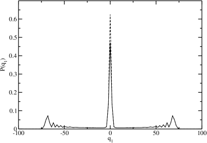
Figure 6: The probability distribution $P(q_{1})$ for detecting at least one walker at position $q_{1}$ after $100$ steps. For initial states $|\psi^{\pm}\rangle$ (dotted line) and $|\phi^{\pm}\rangle$ (solid line), the distribution remains almost same.

For larger number of steps, we do numerical simulations following the method discussed in Sec.IV A. In Fig. 5 the initial states of the photons are maximally entangled states (45) and (46). For different entangled states we get different probability distributions. The differences between the distributions for symmetric states and antisymmetric states are much larger than the differences between the distributions for symmetric-symmetric or antisymmetric-antisymmetric states. Further, we have seen by direct computation that the probability distributions for entangled states can not be reproduced exactly by the walkers having initial states as an incoherent mixture of separable states. In Fig. 6 we have shown the probability distribution $P(q_{1})$ for detecting at least one walker at the position $q_{1}$. In this case the distribution is symmetric for both negative and positive values of $q_{1}$ and has a sharp maxima at initial position $q_{1}=0$. The probability distribution for walkers with maximally entangled initial states (45) and (46) remains almost invariant except at initial position. At initial position the probability of detecting one walker is larger for states (45) than the case of initial state (46). In the case of two-photon QRW with separable Fock states discussed in Sec. IV A, the probability $P(q_{1})$ is different for different initial state. For initial states $|0,0,h,x\rangle\otimes|0,0,v,x\rangle$ and $|0,0,h,y\rangle\otimes|0,0,v,y\rangle$ the distribution $P(q_{1})$ is symmetric on both sides of $q_{1}$-axis and side peaks appears in both positive and negative directions, while in the case of $|0,0,h,x\rangle\otimes|0,0,v,y\rangle$ and $|0,0,h,y\rangle\otimes|0,0,v,x\rangle$ the probability distributions are antisymmetric with one side peak in positive and negative direction respectively.

For large number of steps, we can again use our approximate results (12), (19), (26) and (27) in the following way. For initial state as one of the Bell’s state $|\psi^{\pm}\rangle$ the final state of the photons after $n$ steps will be

$$|\Psi^{\pm}(n)\rangle=\frac{1}{2}\sum_{q_{1},q_{2}=-n}^{n}\left[|\psi_{hx}(n,q_{1})\rangle\otimes|\psi_{vy}(n,q_{2})\rangle+|\psi_{hx}(n,q_{2})\rangle\otimes|\psi_{vy}(n,q_{1})\rangle\right.$$

$$\left.\pm|\psi_{hy}(n,q_{1})\rangle\otimes|\psi_{vx}(n,q_{2})\rangle\pm|\psi_{hy}(n,q_{2})\rangle\otimes|\psi_{vx}(n,q_{1})\rangle\right].$$ (49)

Similarly, for initial state as Bell’s states $|\phi^{\pm}\rangle$, the state of the photons will be

$$|\Phi^{\pm}(n)\rangle=\frac{1}{2}\sum_{q_{1},q_{2}=-n}^{n}\left[|\psi_{hx}(n,q_{1})\rangle\otimes|\psi_{vx}(n,q_{2})\rangle+|\psi_{hx}(n,q_{2})\rangle\otimes|\psi_{vx}(n,q_{1})\rangle\right.$$

$$\left.\pm|\psi_{hy}(n,q_{1})\rangle\otimes|\psi_{vy}(n,q_{2})\rangle\pm|\psi_{hy}(n,q_{2})\rangle\otimes|\psi_{vy}(n,q_{1})\rangle\right].$$ (50)

The results (49) and (50) match very well with exact simulations for large number of steps. Here it should be noted that QRW in our case is different than the case of two entangled walkers discussed in Ref. bose2 . In Ref. bose2 , the correlation between the walkers is completely because of their correlated initial state only. The walkers are nonidentical and evolve completely independent to each other. Thus if the initial state will be a separable state there will be no correlation in QRW and can be produced using walkers in coherent states. It should be borne in mind that we can not construct entangled state of one x-polarized photon and the other y-polarized photon unless some other degree of freedom like direction of propagation is introduced.

VI Conclusions

In conclusion, we have discussed how the quantum features of QRW can be uncovered by studying QRW by photons in a number of quantum states and by detecting the coincidence correlations between two photons. We use two photons, each of which can exist in two polarization states. Further, the photons can travel in either vertical or horizontal direction. The walk is realized by optical elements consisting of polarization beam splitters and half wave plates. We first consider the QRW by a single photon and show how the result of QRW depends on initial state of the photon. A comparison of the Figs.2(a) and 2(b) shows that the probabilities depend on the relative phases in the initial superposition state of the photon. We next consider QRW by two walkers in separable quantum states like Fock states. We show that our optical arrangement entangles two photons even though initially they are in separable states. The joint probability of finding the two photons at two different sites now depends on the initial separable quantum state. Further the probability for single photon detection is different from those calculated in Sec.III. We also examine the QRW of two photons in coherent states. In this case the state of the two photons remains separable. The single photon detection probabilities depend on the initial amplitudes of the two coherent states and thus the interferences are prominent. Finally we consider QRW of two photons in all four Bell states. The resulting joint probability distributions are quite different from those calculated for separable states. All the cases discussed reveal very interesting quantum character. Clearly our analysis is applicable to other systems as well, for example electrons with appropriate arrangement of Stern-Gerlach fields.

Appendix A Fourier Analysis of QRW of a Single Photon

We can write Eq.(7) for the wave function of the single photon in the form

$$\psi(n+1,q)=M_{+}\psi(n,q-1)+M_{-}\psi(n,q+1)$$ (51)

where

$$M_{+}=\frac{1}{\sqrt{2}}\left[\begin{array}[]{cccc}1&1&0&0\\ 0&0&1&-1\\ 0&0&0&0\\ 0&0&0&0\end{array}\right],$$ (56)

$$M_{-}=\frac{1}{\sqrt{2}}\left[\begin{array}[]{cccc}0&0&0&0\\ 0&0&0&0\\ 0&0&1&1\\ 1&-1&0&0\end{array}\right],$$ (61)

and the state of the photon after $n$ steps, $|\psi(n,q)\rangle=c_{hx}|n,q,h,x\rangle+c_{hy}|n,q,h,y\rangle+c_{vx}|n,q,v,x\rangle+c_{vy}|n,q,v,y\rangle$, is expressed in the matrix form

$$\psi(n,q)=\left[\begin{array}[]{c}c_{hx}(n,q)\\ c_{hy}(n,q)\\ c_{vx}(n,q)\\ c_{vy}(n,q)\end{array}\right].$$ (62)

Now we solve Eq.(51) using spatial discrete Fourier transform. The spatial discrete Fourier transform for $k\in[-\pi,\pi]$ is defined by

$$\tilde{\psi}(k)=\sum_{x}\psi(x)e^{ikx},$$ (63)

$${\rm and}~{}\psi(x)=\frac{1}{2\pi}\int_{-\pi}^{\pi}\tilde{\psi}(k)e^{-ikx}dk.$$ (64)

We write Eq.(51)in the Fourier domain using transform (63) as following,

$$\tilde{\psi}(n+1,k) = \sum_{x}M_{+}\psi(n,x-1)e^{ikx}+M_{-}\psi(n,x+1)e^{ikx}$$ (65)

$$= (e^{ik}M_{+}+e^{-ik}M_{-})\tilde{\psi}(n,k)$$

$$= M_{k}\tilde{\psi}(n,k)$$

where

$$M_{k}=\frac{1}{\sqrt{2}}\left[\begin{array}[]{cccc}e^{ik}&e^{ik}&0&0\\ 0&0&e^{ik}&-e^{ik}\\ 0&0&e^{-ik}&e^{-ik}\\ e^{-ik}&-e^{-ik}&0&0\end{array}\right].$$ (66)

It is clear from Eq.(65) that in the Fourier domain the $n$ step QRW of the photon starting from the state $\tilde{\psi}(0,k)$ is given by

$$\tilde{\psi}(n,k) = (M_{k})^{n}\tilde{\psi}(0,k)$$ (67)

$$= \sum_{m}(\lambda_{m})^{n}|\Phi_{m}\rangle\langle\Phi_{m}|\tilde{\psi}(0,k)\rangle$$

where $\lambda_{m}$ and $\Phi_{m}$ are eigenvalue and corresponding eigenvector of $M_{k}$. Thus, we can calculate exact value of $\tilde{\psi}(n,k)$ by diagonalizing $M_{k}$ and writing initial state of the photon in Fourier domain. The state of the photon after $n$ steps in original domain $\psi(n,q)$ is given by the inverse Fourier transform of $\tilde{\psi}(n,k)$, defined by Eq.(64). The eigenvalues of $M_{k}$ are $\lambda_{1}=-1$, $\lambda_{2}=1$, $\lambda_{3}=e^{-i\omega_{k}}$ and $\lambda_{4}=e^{i\omega_{k}}$, where $\omega_{k}\in[\pi/4,3\pi/4]$ and defined as $\cos\omega_{k}=\cos k/\sqrt{2}$. The corresponding eigenvectors are

$$|\Phi_{1}\rangle=\frac{1}{2}\sqrt{\frac{3+2\sqrt{2}\cos k}{2+\sqrt{2}\cos k}}\left[\begin{array}[]{c}\frac{-e^{ik}}{\sqrt{2}+e^{-ik}}\\ \frac{\sqrt{2}+e^{ik}}{\sqrt{2}+e^{-ik}}\\ \frac{-e^{-ik}}{\sqrt{2}+e^{-ik}}\\ 1\end{array}\right],$$ (72)

$$|\Phi_{2}\rangle=\frac{1}{2}\sqrt{\frac{3-2\sqrt{2}\cos k}{2-\sqrt{2}\cos k}}\left[\begin{array}[]{c}\frac{e^{ik}}{\sqrt{2}-e^{-ik}}\\ \frac{\sqrt{2}-e^{ik}}{\sqrt{2}-e^{-ik}}\\ \frac{e^{-ik}}{\sqrt{2}-e^{-ik}}\\ 1\end{array}\right],$$ (77)

$$|\Phi_{3}\rangle=\frac{1}{2\sqrt{1+\sin^{2}k}}\left[\begin{array}[]{c}-1+\sqrt{2}e^{-i(\omega_{k}-k)}\\ -1\\ 1-\sqrt{2}e^{-i(\omega_{k}+k)}\\ 1\end{array}\right],$$ (82)

$$|\Phi_{4}\rangle=\frac{1}{2\sqrt{1+\sin^{2}k}}\left[\begin{array}[]{c}-1+\sqrt{2}e^{i(\omega_{k}+k)}\\ -1\\ 1-\sqrt{2}e^{i(\omega_{k}-k)}\\ 1\end{array}\right].$$ (87)

If the initial state of the photon is $|0,0,h,x\rangle$ the corresponding state in fourier domain will be $\tilde{\psi}(0,k)=[1,0,0,0]^{T}$ for all values of $k$. Similarly if the photon starts QRW from state $|0,0,h,y\rangle$ the initial state in Fourier domain will be $[0,1,0,0]^{T}$. Now from Eq.(67), we calculate the state of the quantum walker $\tilde{\psi}(n,k)$ in fourier domain. Taking the inverse Fourier transform of $\tilde{\psi}(n,k)$, we get the state of the walker after $n$ steps $\psi(n,q)$ in the original coordinate space. For initial state of the photon $|0,0,h,x\rangle$, we get

$$|\psi_{hx}(n,q)\rangle=f_{hx}|n,q,h,x\rangle+f_{hy}|n,q,h,y\rangle+f_{vx}|n,q,v,x\rangle+f_{vy}|n,q,v,y\rangle,$$ (88)

where the coefficients $f_{\alpha\beta}$ are given by

$$f_{hx}=\frac{1+(-1)^{n+q}}{8\pi}\left[\int_{-\pi}^{\pi}\frac{\cos(kq)}{2-\sqrt{2}\cos k}dk+\int_{-\pi}^{\pi}\frac{3-2\sqrt{2}\cos(\omega_{k}-k)}{1+\sin^{2}k}e^{-i(n\omega_{k}+kq)}dk\right],$$ (89)

$$f_{hy}=\frac{1+(-1)^{n+q}}{8\pi}\left[\int_{-\pi}^{\pi}\frac{\sqrt{2}\cos[k(q+1)]-\cos(kq)}{2-\sqrt{2}\cos k}dk+\int_{-\pi}^{\pi}\frac{1-\sqrt{2}e^{i(\omega_{k}-k)}}{1+\sin^{2}k}e^{-i(n\omega_{k}+kq)}dk\right],$$ (90)

$$f_{vx}=\frac{1+(-1)^{n+q}}{8\pi}\left[\int_{-\pi}^{\pi}\frac{\cos[k(q+2)]}{2-\sqrt{2}\cos k}dk-\int_{-\pi}^{\pi}\frac{e^{-2ik}}{1+\sin^{2}k}e^{-i(n\omega_{k}+kq)}dk\right],$$ (91)

$$f_{vy}=\frac{1+(-1)^{n+q}}{8\pi}\left[\int_{-\pi}^{\pi}\frac{\sqrt{2}\cos[k(q+1)]-\cos[k(q+2)]}{2-\sqrt{2}\cos k}dk+\int_{-\pi}^{\pi}\frac{\sqrt{2}e^{i(\omega_{k}-k)}-1}{1+\sin^{2}k}e^{-i(n\omega_{k}+kq)}dk\right].$$ (92)

Similarly, for initial state of the photon $|0,0,h,y\rangle$, the state of the walker after $n$ steps is

$$|\psi_{hy}(n,q)\rangle=g_{hx}|n,q,h,x\rangle+g_{hy}|n,q,h,y\rangle+g_{vx}|n,q,v,x\rangle+g_{vy}|n,q,v,y\rangle,$$ (93)

where

$$g_{hx}=\frac{1+(-1)^{n+q}}{8\pi}\left[\int_{-\pi}^{\pi}\frac{\sqrt{2}\cos[k(q-1)]-\cos(kq)}{2-\sqrt{2}\cos k}dk+\int_{-\pi}^{\pi}\frac{1-\sqrt{2}e^{-i(\omega_{k}-k)}}{1+\sin^{2}k}e^{-i(n\omega_{k}+kq)}dk\right],$$ (94)

$$g_{hy}=\frac{1+(-1)^{n+q}}{8\pi}\left[\int_{-\pi}^{\pi}\frac{(3-2\sqrt{2}\cos k)\cos(kq)}{2-\sqrt{2}\cos k}dk+\int_{-\pi}^{\pi}\frac{e^{-i(n\omega_{k}+kq)}}{1+\sin^{2}k}dk\right],$$ (95)

$$g_{vx}=\frac{1+(-1)^{n+q}}{8\pi}\left[\int_{-\pi}^{\pi}\frac{\sqrt{2}\cos[k(q+1)]-\cos[k(q+2)]}{2-\sqrt{2}\cos k}dk+\int_{-\pi}^{\pi}\frac{\sqrt{2}e^{-i(\omega_{k}+k)}-1}{1+\sin^{2}k}e^{-i(n\omega_{k}+kq)}dk\right],$$ (96)

$$g_{vy}=\frac{1+(-1)^{n+q}}{8\pi}\left[\int_{-\pi}^{\pi}\frac{2\cos kq-2\sqrt{2}\cos[k(q+1)]+\cos[k(q+2)]}{2-\sqrt{2}\cos k}dk-\int_{-\pi}^{\pi}\frac{e^{-i(n\omega_{k}+kq)}}{1+\sin^{2}k}dk\right].$$ (97)

Because of the factor $1+(-1)^{n+q}$, coefficients $f_{\alpha\beta}$ and $g_{\alpha\beta}$ are nonzero for even values of $n+q$ only, which is corresponding to the positions of detecting photon in the arrangement (see Fig.1) for a fixed value of $n$. The integrals inside the bracket can not be evaluated exactly. Further the first integral inside the bracket is independent of $n$, and is responsible for the constant spikes in the probability of detecting photon near the initial position $q=0$. The second integral inside the bracket completely characterizes QRW.

In order to understand the nature of QRW we do asymptotic analysis of the second integral inside the bracket in the coefficients $f_{\alpha\beta}$ and $g_{\alpha\beta}$ as follows. The integral has the form of

$$I(n)=\int_{-\pi}^{\pi}f(k)e^{in\phi(k)}dk,$$ (98)

where $\phi(k)=-(\omega_{k}+k\alpha)$, $\alpha=q/n$, and $f(k)$ is function of $k$ only. In the limit of large $n$ we use stationary phase approximation bornwolf and find the approximate value of $I(n)$.

$$I(n)\approx\sqrt{\frac{2\pi}{n|\phi^{\prime\prime}(k_{0})|}}\Re\left\{f(k_{0})e^{in\phi(k_{0})-i\pi/4}\right\},~{}{\rm for~{}}-\frac{1}{\sqrt{2}}<\alpha<\frac{1}{\sqrt{2}},$$ (99)

where $k_{0}=\sin^{-1}(-\alpha/\sqrt{1-\alpha^{2}})$ and prime denotes the derivative with respect to $k$. For $\alpha=\pm 1/\sqrt{2}$, $\phi(k)$ has stationary point of order two at $k=\pm\pi/2$, i.e. $\phi^{\prime}(\pm\pi/2)=0,~{}\phi^{\prime\prime}(\pm\pi/2)=0,~{}\phi^{\prime\prime\prime}(\pm\pi/2)\neq 0$. At these points

$$I(n)\approx\left(\frac{6}{n}\right)^{1/3}\frac{\sqrt{2}\Gamma(1/3)}{\sqrt{3}}f(-\pi/2)e^{in\phi(-\pi/2)},~{}{\rm for~{}}\alpha=\frac{1}{\sqrt{2}},$$ (100)

$$I(n)\approx\left(\frac{6}{n}\right)^{1/3}\frac{\sqrt{2}\Gamma(1/3)}{\sqrt{3}}f(\pi/2)e^{in\phi(\pi/2)},~{}{\rm for~{}}\alpha=-\frac{1}{\sqrt{2}}.$$ (101)

Everywhere else $I(n)$ has no stationary point and averages to zero for $n\rightarrow\infty$.

References

• (1) Y. Aharonov, L. Davidovich, and N. Zagury, Phys. Rev. A 48, 1687 (1993).
• (2) B. C. Sanders, S. D. Bartlett, B. Tregenna, and P. L. Knight, Phys. Rev. A 67, 042305 (2003); V. Kendon and B. C. Sanders, Phys. Rev. A 71, 022307 (2005) .
• (3) T. Di, M. Hillery, and M. S. Zubairy, Phys. Rev. A 70, 032304 (2004); M. Hillery, J. Bergou, and E. Feldman, Phys. Rev. A 68, 032314 (2003).
• (4) B. C. Travaglione and G. J. Milburn, Phys. Rev. A 65, 032310 (2002).
• (5) C. A. Ryan, M. Laforest, J. C. Boileau, and R. Laflamme, Phys. Rev. A 72, 062317 (2005).
• (6) P. Ribeiro, P. Milman, and R. Mosseri, Phys. Rev. Lett. 93, 190503 (2004).
• (7) J. Kempe, Contemp. Phys. 44, 307 (2003).
• (8) B. Do, M. L. Stohler, S. Balasubramanian, D. S. Elliott, C. Eash, E. Fischbach, M. A. Fischbach, A. Mills, B. Zwickl, J. Opt. Soc. Am. B, 22, 499 (2005).
• (9) Z. Zhao, J. Du, H. Li, T. Yang, Z.-B. Chen, and J.-W. Pan, e-print quant-ph/0212149.
• (10) H. Jeong, M. Paternostro, and M. S. Kim, Phys. Rev. A 69 , 012310 (2004).
• (11) P. L. Knight, E. Roldan, and J. E. Sipe, Phys. Rev. A 68, 020301(R) (2003); Opt. Commun. 227, 147 (2003).
• (12) I. Carneiro, M. Loo, X. Xu, M. Girerd, V. Kendon, and P. L. Knight, New J. Phys. 7, 156 (2005).
• (13) D. Bouwmeester, I. Marzoli, G. P. Karman, W. Schleich, and J. P. Woerdman, Phys. Rev. A 61, 013410 (2000).
• (14) G. S. Agarwal and P. K. Pathak, Phys. Rev. A 72, 033815 (2005).
• (15) S. E. Venegas-Andraca, J. L. Ball, K. Burnett, and S. Bose, New J. Phys. 7, 221 (2005).
• (16) Y. Omar, N. Paunkovic, L. Sheridan, S. Bose, e-print quant-ph/0411065.
• (17) W. Dür, R. Raussendorf, V. M. Kendon, and H. -J. Briegel, Phys. Rev. A 66, 052319 (2002); K. Eckert, J. Mompart, G. Birkl, M. Lewenstein, Phys. Rev. A 72, 012327 (2005).
• (18) C. K. Hong, Z. Y. Ou, and L. Mandel, Phys. Rev. Lett. 59, 2044 (1987); Z. Y. Ou and L. Mandel, Phys. Rev. Lett. 61, 50 (1988); R. Ghosh and L. Mandel, Phys. Rev. Lett. 59, 1903 (1987).
• (19) P. G. Kwiat, K. Mattle, H. Weinfurter, A. Zeilinger, A. V. Sergienko, and Y. Shih, Phys. Rev. Lett. 75, 4337 (1995).
• (20) A. Nayak and A. Vishwanath, e-print quant-ph/0010117.
• (21) T. A. Brun, H. A. Carteret, and A. Ambainis, Phys. Rev. A 67, 052317 (2003); Phys. Rev. Lett. 91, 130602 (2003).
• (22) J. L. O’Brien, G. J. Pryde, A. G. White, T. C. Ralph, D. Branning, Nature (London)426, 264 (2003).
• (23) J. T. Barreiro, N. K. Langford, N. A. Peters, and P. G. Kwiat, Phys. Rev. Lett. 95, 260501 (2005); F. A. Bovino, G. Castagnoli, A. Ekert, P. Horodecki, C. M. Alves, and A. V. Sergienko, ibid. 95, 240407 (2005).
• (24) R. J. Glauber, Phys. Rev. 131, 2766 (1963).
• (25) L. Mandel and E. Wolf, in Optical Coherence and Quantum Optics (Cambridge University Press, 1995) p.128.