Universal decoherence induced by an environmental quantum phase transition
Abstract
Decoherence induced by coupling a system with an environment may display universal features. Here we demostrate that when the coupling to the system drives a quantum phase transition in the environment, the temporal decay of quantum coherences in the system is Gaussian with a width independent of the system-environment coupling strength. The existence of this effect opens the way for a new type of quantum simulation algorithm, where a single qubit is used to detect a quantum phase transition. We discuss possible implementations of such algorithm and we relate our results to available data on universal decoherence in NMR echo experiments.
The coupling between a quantum system and its environment leads to decoherence, the process by which quantum information is degraded. Decoherence plays a crucial role in the understanding of the quantum to classical transition deco . It also has practical importance: its understanding is essential in technologies that actively use quantum coherence, such as quantum information processing QIP . In general, the timescale of decoherence depends on the system-environment coupling strength, which we arbitrarily denote . For example, in the well studied case of quantum Brownian motion (where the environment consists of a large number of non–interacting harmonic oscillators), quantum coherence generally decays exponentially with a rate proportional to qbm . In this letter we describe a class of systems with a drastically different behavior: Gaussian decay of coherence with a rate independent of . This independence signals a universal behavior whose study is the aim of this work. In general, one should avoid building physical quantum information processing devices in presence of universal decoherence. However, we show that universality is a powerful property we can use to our advantadge: by detecting decoherence in the universal regime we can extract valuable information about the environment.
Environment-independent decoherence rates are also found in other circumstances. For example, systems with a classically chaotic Hamiltonian display a “Lyapunov regime” where the decay is exponential and given by the Lyapunov exponent of the underlying classical dynamics ZurekPaz ; Lecho1 . These models are also often used to represent a complex environment. In fact, chaoticity is the widespread explanation Lecho1 ; Lecho2 for the perturbation-independent decay of polarization detected in recent NMR echo experiments Horacio (where, however, a non-exponential but Gaussian decay is actually observed). Our findings are different from the usual exponential Lyapunov regime: we discuss systems where the universal (independent of ) decoherence is Gaussian. In our model, the complexity and sensitivity of the environment arise from the susceptibility of the environmental spectrum to the system’s state. The relation between our results and the experiments of Ref. Horacio will also be discussed below.
Let us consider a spin particle (a qubit) coupled to an environment that is “structurally unstable” with respect to the system state (in a sense that will be made clear below). The model we discuss is a generalization of the one studied by Quan et al Quan , who showed that an environment at the critical point of a quantum phase transition is highly efficient in producing decoherence. Below, we will not only generalize the results of Quan but also show that in these circumstances universal decoherence arises naturally. We assume that the system and the environment evolve under the Hamiltonian
| (1) |
Here, the operators , and act on the Hilbert space of the environment. If the system is in state (), the environment evolves with an effective Hamiltonian ( is the system-environment coupling strength). Considering the initial state the evolved reduced density matrix of the system is
| (2) | |||||
The off-diagonal terms of this operator are modulated by the decoherence factor : the overlap between two states of the environment obtained by evolving the initial state with two different Hamiltonians, i.e. . Moreover, assuming that the initial state of the environment is the ground state of eigenstate , the decoherence factor is, up to an irrelevant phase factor, identical to the so–called survival probability amplitude
| (3) |
Let us first analyze models where both Hamiltonians () can be diagonalized in terms of a suitable set of fermionic creation and annihilation operators :
| (4) |
Furthermore, we assume that the operators appearing in the two Hamiltonians can be connected by a Bogoliubov transformation of the form
| (5) |
where the angles define the Bogoliugov coefficients. Notice that this expression only includes mixing between modes with opposite values of the index . Our treatment can be extended to more complicated situations, but we limit first to the simplest non–trivial case, where it is possible to relate the ground states of as
| (6) |
Under these assumptions the decoherence factor is
| (7) |
Surprisingly, is completely analogous to the one found when studying non–interacting spin environments Cucchietti . In that case, the index labels the different environmental spins and the corresponding Bogoliubov coefficients define their initial states.
Under reasonable assumptions on the angles and the energies , we can go further and – using the ideas developed in Cucchietti – obtain a simple form for the temporal evolution of the overlap . To illustrate our procedure, let us analyze first an oversimplified case: suppose that the energies of all the modes are the same, i.e. . In the simplest case , the overlap oscillates as . The same result is recovered as a consecuence of the law of large numbers if the angles are spread over the entire circle. In fact, if the following Lindenberg conditions are satisfied
| (8) |
The first condition is satisfied when the angles are randomly distributed. The second one imposes a finite variance for the “quantum walk” in which a step of length () is taken with probability (). When , the condition takes the form , and it is met when there is a sufficiently large number of modes for which does not vanish.
A more realistic situation is when the energies take values in a given spectral band. When the energies are distributed with a vanishing mean value, the decay of is Gaussian with a width given by defined in (8) Cucchietti . Consider the more general case where the energies are distributed about an arbitrary mean value, i.e. (where has zero mean). We now define the dispersion as the cumulative variance of the fluctuations of the energy, i.e. . We find that, in general, when conditions (8) hold (replacing by ), is described by a Gaussian envelope modulating an oscillating term,
| (9) |
In general, when the operators and are similar, the angles are small and (8) do not hold: there is almost no decoherence. However, a drastic difference in the nature of the eigenstates of and can only be accounted for with varying in the full range . This occurs when the environment suffers a quantum phase transition when is varied. Thus, denoting the critical point of the transition, for we expect the decoherence factor to behave as indicated in (9). In many cases, is only given by the properties of the environment Hamiltonian, and thus the decay of becomes universal (independent of ).
An important model encompassed by assumptions (4) and (5) is an Ising chain transversely coupled to a central spin Quan (which plays the role of the system). In this case
| (10) |
The Bogoliubov coefficients and the energies are Sachdev ,
| (11) | |||||
| (12) |
where the angles are defined from . In this model .
When and , the angles and the Bogoliubov coefficients satisfy conditions (8). Moreover, the energies are distributed between and , which gives . Therefore, the width of the Gaussian envelope is independent of .

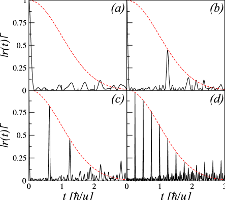
In Fig. 1 we display for the case , showing the accuracy of Eq. (9). The universality of the envelope is a clear indication of the quantum phase transition. However, the oscillations (whose frequency depends on ) are not universal. Yet, it is possible to eliminate them by performing a spin-echo experiment: first, evolve the system coupled to the Ising chain environment for a time . At this time, flip the environmental spins in the direction (e.g. with an rf-pulse that applies a -rotation around the -axis). Finally, evolve for another time . The total evolution of the environment can be described by using the Hamiltonian from time to , and from time to . Thus, in this echo experiment the decoherence factor is given by
| (13) |
This overlap is simply computed using the Bogoliubov transformation that connect the modes diagonalizing the Hamiltonians and . If we denote the modes of , the Bogoliubov coefficients associated with the corresponding angles are such that . The analytic form for the overlap is simplified introducing the sum and difference of the energies, , and the Bogoliubov angles, . We obtain
| (14) | |||||
For the case of the Ising model the expression can be evaluated explicitely. In the limit of large values of , one can obtain an approximate behavior using similar arguments as above remark . Thus, the dominant contribution to the echo–overlap is
| (15) |
where . In Fig. 1 we show how the accuracy of this expression increases with .
To test the generality of our results against the restrictiveness and uncontrollability of assumptions (4) and (5), we study a system in the opposite end of the spectrum: the Bose-Hubbard model (BHM) Sachdev , with Hamiltonian
| (16) |
Here are boson anihilation operators in site of a discrete lattice. For , the system behaves as a superfluid of non–interacting particles. In the opposite regime, , the interaction term dominates and the ground state is Mott-insulator like. This model cannot be cast in terms of fermionic operators as in (4), in fact, no analytic solution is known. Furthermore, the bosonic nature of the particles also conflicts with (5). The BHM has practical relevance because it can be experimentally simulated using cold neutral atoms in an optical lattice Bloch . We calculate numerically for a spin coupled to the hopping term of the BH Hamiltonian, that is, we take . In Fig. 2 we show the decoherence factor for several values of for a BHM with a fixed number of bosons. The same overall behavior of the Ising chain is observed: a universal Gaussian envelope (independent of ) modulating an oscillation with frequency proportional to . The very different nature of the BHM hints at a more general validity of our results.
A Gaussian decay of coherence with a rate independent of the coupling to the environment was indeed observed in NMR polarization echo experiments Horacio . Arguing on the complexity of the experimental many-body system, these results have been related to the environment-independent decoherence predicted in classically chaotic Hamiltonians ZurekPaz ; Lecho1 ; Lecho2 . The experimental situation is quite different from the one we considered here: the decoherence factor is measured after an echo created by a change of sign of the environment Hamiltonian, and not the system-bath interaction. Our model points to a different way of introducing complexity and sensitivity in the environment: a quantum phase transition. Further research using this approach might explore more realistic models that account for all the details of the experiments.
The universal decoherence regime of this work can also be understood using analogies to the regime of strong perturbations of the survival probability, Eq. (3). Indeed, is the Fourier transform of the strength function or local density of states (LDOS), , where are the eigenvectors of and its eigenenergies. In typical LDOS studies, differs from by a perturbation. In complex systems (e.g. random matrices, or classically chaotic Hamiltonians) for sufficiently strong perturbations is a random superposition of the states. Therefore, the LDOS becomes independent of the perturbation: it equals the full density of states of . In our model, the saturation of the LDOS when and are on both sides of the quantum phase transition occurs because of the radically different nature of the eigenstates. In contrast to our results, Refs. Heller have found that complex systems give an LDOS with a Lorentzian shape, leading to an exponential decay of .
Universal decoherence can be harmful for quantum information applications. However, it can be a useful tool to extract information about a critical system, e.g. its spectral structure or the critical point of its quantum phase transition. The latter example can be thought of as a “critical point finding” algorithm in a one-qubit quantum computer: in systems where the spectrum is not shifted by the coupling (which gives the oscillatory term), the critical point can be simply obtained as the value for which one observes the onset of universality. Otherwise, the oscillation term obscures the critical point. In these cases one can instead couple the system weakly to the environment, and drive the transition with an external parameter (as in Ref. Quan ). The critical point is then signaled by the value for which there is a maximum decoherence decay. A demonstration of this algorithm can be performed in an NMR setting simulating the Ising Hamiltonian studied above Raymond .
We have shown that when the coupling to the system drives a quantum phase transition in the environment, the decoherence factor decays as a Gaussian with an environment-independent width. We showed numerically that our findings are more general than what can be expected from the analytical approximations we used. Our results could lead to an alternative interpretation of hitherto unexplained NMR experimental results on environment independent decoherence rates. Finally, we discussed how the universal behavior of the decoherence factor can be used to study critical systems in a novel simulation algorithm for one-qubit quantum computers. We acknowledge fruitful discussions with W.H. Zurek.
References
- (1) J. P. Paz and W. H. Zurek, in Coherent matter waves, Les Houches Session LXXII, R Kaiser, C Westbrook and F David eds., EDP Sciences (Springer Verlag, Berlin, 2001) 533-614; W.H. Zurek, Rev. Mod. Phys. 75, 715 (2003).
- (2) M. A. Nielsen and I. L. Chuang, Quantum computation and quantum information (Cambridge University Press, Cambridge, New York, 2000).
- (3) B.L. Hu, J.P. Paz, and Y. Zhang, Phys. Rev. D 45, 2843 (1992).
- (4) W.H. Zurek and J.P. Paz, Phys. Rev. Lett. 72, 2508 (1994).
- (5) R.A. Jalabert and H.M. Pastawski, Phys. Rev. Lett. 86, 2490 (2001).
- (6) F.M. Cucchietti, H.M. Pastawski, and R.A. Jalabert, Phys. Rev. B 70, 035311 (2004).
- (7) H.M. Pastawski, P.R. Levstein, G. Usaj, J. Raya, and J. Hirschinger, Physica A 283, 166 (2000).
- (8) H.T. Quan, Z. Song, X.F. Liu, P. Zanardi, and C.P. Sun, quant-ph/0509007.
- (9) Any eigenstate of results in the same expression.
- (10) F.M. Cucchietti, J.P. Paz, and W.H. Zurek, Phys. Rev. A 72, 052113 (2005).
- (11) S. Sachdev, Quantum Phase Transitions (Cambridge University Press, Cambridge, 1999).
- (12) For the solution of has to be taken from the second branch of the tangent, , to satisfy the symmetries of the Ising Hamiltonian (10), giving .
- (13) M. Greiner et al., Nature (London) 419, 51 (2002).
- (14) E.P. Wigner, Ann. Math. 62, 548 (1955); 65, 203 (1957); Ph. Jacquod and D.L. Shepelyansky, Phys. Rev. Lett. 75, 3501 (1995); D. Cohen and E.J. Heller, Phys. Rev. Lett. 84, 2841 (2000).
- (15) R. Laflamme, private communication.