Fields of Iterated Quantum Reference Frames based on Gauge Transformations of Rational String States

Abstract

This work is based on a description of quantum reference frames that seems more basic than others in the literature. Here a frame is based on a set of real and of complex numbers and a space time as a 4-tuple of the real numbers. There are many isomorphic frames as there are many isomorphic sets of real numbers. Each frame is suitable for construction of all physical theories as mathematical structures over the real and complex numbers. The organization of the frames into a field of frames is based on the representations of real and complex numbers as Cauchy operators defined on complex rational states of finite qubit strings.

The structure of the field is based on noting that the construction of real and complex numbers as Cauchy operators in a frame can be iterated to create new frames coming from a frame. Gauge transformations on the rational string states greatly expand the number of quantum frames as, for each gauge U, there is one frame coming from the original frame. Forward and backward iteration of the construction yields a two way infinite frame field with satisfying properties. There is no background space time and there are no real or complex numbers for the field as a whole. Instead these are relative concepts associated with each frame in the field. Extension to include qukit strings for different k bases, is described as is the problem of reconciling the frame field to the existence of just one frame with one background space time for the observable physical universe.

I Introduction

As is well known, real and complex numbers are very important to physics. All physical theories can be described as mathematical structures erected over the real and complex numbers. All theoretical predictions can be represented as real number solutions to equations given by the theories. Also in many of the theories space time is represented as a $4$ tuple (or D-tuple in string theories) of the real numbers with an associated topology or metric structure.

Another basic aspect of physics is that all physical representations of integers and rational numbers consist of a finite string of physical systems in states that correspond to a $k-ary$ representation of a number. Examples include the binary string representation of numbers used in most computations and computers, and the numerical output of measurements as finite strings of decimal digits. The string representation is also used in languages where words are strings of symbols in some alphabet.

These aspects emphasize the importance of real numbers. Complex numbers are ordered pairs of real numbers with appropriate rules for addition and multiplication of the pair components. A 4 tuple of real numbers is the representational basis for space time with topologies or metric structures added as appropriate. Also emphasized is the importance of finite strings of kits or qukits as $k-ary$ representations of rational number approximations to real and complex numbers. These will play a basic role here.

Another aspect of central importance here is that there are many different reference frames in quantum theory Aharonov . They play an important role in quantum security protocols where a sender and receiver choose a reference frame for transmission and receipt of quantum information Bagan ; Rudolph ; Bartlett ; vanEnk .

In this paper reference frames play a much more basic role than has been used so far. In work done to date, such as that referenced above and Enk , different reference frames are described within a fixed background space time. They are also based on a fixed set of real and complex numbers. Here each reference frame is defined by or based on sets of real numbers, $R,$ and complex numbers, $C,$ and $R^{4}$ as a basis of space time. The choice of topology and additional structure on $R^{4}$ depends on the theory being considered in the frame.

Since there are many different isomorphic representations of the real numbers there are many different isomorphic frames. Each frame is equivalent in that physical theories constructible by an observer in any one frame should have their equivalents in any other frame. This includes all theories that are mathematical structures over the real and complex numbers and describe the dynamics of systems in the background space time.

If all these frames were not related and were independent of one another, this result would be of very limited interest. However this is not the case. The different frames are related. They form a structure that is a field of iterated quantum frames over the local and global gauge transformations of complex rational string states.

The goal of this paper is to describe this structure and some of its properties. The structure is based on the quantum theory definitions of real and complex numbers as (equivalence classes of) Cauchy operators. The definition of these operators is based on that for Cauchy sequences of real or complex rational string states BenRRCNQT . These are states of finite qubit (or qukit) strings that are the quantum equivalent of the representation of real or complex rational numbers as finite digit strings in the binary (or $k-ary$) basis.

The iteration of frames arises from the observation that in any frame, finite complex rational string states can be defined along with a set of Cauchy operators on these states. Since these Cauchy operators are real and complex numbers, they form the basis of another frame with a space time basis as a $4-tuple$ of the real number operators. This frame can be said to come from or emanate from the original frame. Since this process can be iterated one ends up with a finite, one way infinite, or two way infinite structure of iterated quantum frames.

This one dimensional structure of iterated frames becomes two dimensional when one notes that there are a large number of representations of complex rational string states related by global Enk and local gauge transformations on the qubit string states. Extension of the structure to show the large number of different frames, one for each gauge transformation, coming from a frame, gives the resulting field structure of quantum frames.

Most of this paper is devoted to describing and understanding various aspects of this structure. The next section gives a representation of complex binary rational string states in terms of products of qubit creation operators acting on a vacuum state. Basic arithmetic relations and operations are described. Section III repeats the definition in BenRRCNQT of Cauchy sequences of complex binary rational string states and uses it to define operators that satisfy a corresponding Cauchy condition. The real and complex number status of sets of Cauchy operators is based on noting that the proofs given in BenRRCNQT can be applied here.

Gauge transformations, as products of unitary operators in $SU(2),$ are introduced in Section IV. Transformations of rational string states and of the basic arithmetical relations and operations are described. Transformed Cauchy operators and the transformed Cauchy condition that they satisfy are also described.

Section V uses these results to describe the basic structure of frames emanating from frames and the frame fields. The relation between observers in adjacent frames is discussed. Section VI completes the structure description by expanding it to include number strings to any base. It is seen that in this case each qukit operator in a gauge transformation can be represented as a product of operators in $U(1)\times SU(2)\times\cdots\times SU(p_{m}).$ Here $p_{m}$ is the $mth$ prime number.

The next section addresses the fundamental question of the connection of the structure to physics. The main problem is how to reconcile the infinity of reference frames, each with its own numbers and space time arena, to the physical existence of just one space time arena for physical systems ranging from cosmological to microscopic. In essence the problem is that all frames in the frame field are isomorphic or unitarily equivalent. But they are not the same.

The solution of this problem is left to future work. However, it is noted that this requires some sort of process of merging or collapsing the frames into one frame, either by direct steps or by some limiting process so that the frames all become the same frame in the limit. Possible approaches include use of quantum error correction code methods, particularly those of decoherence free subspaces Lidar . An example of how this might work is briefly summarized.

It is clear that much work remains to be done. However, the frame field picture is quite satisfactory in many ways. For the two way infinite field there is no absolute concept of given or abstract real or complex numbers. As is the case with loop quantum gravity Smolin , there is no background space time associated with the frame field as a whole. These are relative concepts only in that for an observer in a frame, the real and complex numbers are abstract and the frame space time is the background. However, they are different for different frames. Also the frame tree has a basic direction built in, that of frames coming from frames. This picture also provides some concrete steps towards the construction of a coherent theory of physics and mathematics together BenTCTPM .

Another advantage of this approach is that it may provide a new approach to resolution of outstanding physical problems such as the integration of gravity with quantum mechanics. The new approach is based on the possibility that what an observer in a frame $F$ sees as quantum dynamics of qubit string systems in states that represent numbers, and the corresponding dynamics of Cauchy operators, may be interpreted by an observer in a frame coming from $F$ as properties of his space time. This would avoid the problem of an observer having to reconcile quantum mechanical aspects of systems and gravity for the same space time background of his own frame. In this approach it is possible that quantum dynamics of some systems in one frame correspond to metric and topological properties of space time in another frame.

If one regards complex numbers as ordered pairs of real numbers and space time as based on a 4 tuple of real numbers, then real numbers can be considered as the basis of the whole frame field construction. However complex numbers are basic because physical theories are mathematical structures over the complex numbers. Also a space time arena is needed for any theory describing the dynamics of systems moving in space time. A theory such as loop quantum gravity Smolin ; Rovelli , which is space time background independent, can be in any of the frames by ignoring the space time part of the frame. Aspects of string theory that emphasize the emergent properties of space times and the connections to general relativity Horowitz may be relevant.

Here complex numbers will be built directly by working with complex rational number states of qubit strings described by two types of annihilation creation operators, one for real and one for imaginary rational number states. In this way both components of complex numbers will be built up together rather than first building real numbers and then describing complex numbers as ordered pairs of real numbers.

There does not appear to have been much study of quantum theory representations of real or complex numbers. The first mention of representations of real numbers as Hermitian operators appeared in the 1980s in a study of Boolean valued models of ZF set theory Takeuti and appears to have been studied briefly at that time Davis ; Gordon . Other more recent work on quantum representations of real numbers includes that in BenRRCNQT and Litvinov ; Corbett ; Tokuo . Of special note is recent work that emphasizes the possible importance of different sets of real numbers based on Takeuti’s work in a category theoretic setting Krol .

II Real and Complex Binary Rational String States

There are a great many ways to represent real, imaginary, and complex binary rational string numbers in quantum theory. Here a representation based on annihilation creation operators for qubits is used that is different from that in BenRRCNQT and BenRCRNQM in that both the $0s$ and $1s$ will be included. This coincides with the usual descriptions of quantum information as $0-1$ string states of qubit strings.

Let $a_{\alpha,j}$ and $a^{{\dagger}}_{\alpha,j}$ where $\alpha=0,1$ and $j=\cdots,-1,0,1,\cdots$ be annihilation creation (AC) operators for one type of system in state $\alpha$ at integer site $j.$ Similarly let $b_{\beta,j}$ and $b^{{\dagger}}_{\beta,j}$ be AC operators for another type of system in state $\beta=0,1$ at site $j$. For bosons or fermions the AC operators satisfy commutation or anticommutation relations respectively:

$$\begin{array}[]{c}[a_{\alpha,j},a^{{\dagger}}_{\alpha^{\prime},j^{\prime}}]=\delta_{j,j^{\prime}}\delta_{\alpha,\alpha^{\prime}}\\ \mbox{$[a^{{\dagger}}_{\alpha,j},a^{{\dagger}}_{\alpha^{\prime},j^{\prime}}]=[a_{\alpha,j},a_{\alpha^{\prime},j^{\prime}}]=0$}\end{array}$$ (1)

or

$$\begin{array}[]{c}\{a_{\alpha,j},a^{{\dagger}}_{\alpha^{\prime},j^{\prime}}\}=\delta_{j,j^{\prime}}\delta_{\alpha,\alpha^{\prime}}\\ \{a^{{\dagger}}_{\alpha,j},a^{{\dagger}}_{\alpha^{\prime},j^{\prime}}\}=\{a_{\alpha,j},a_{\alpha^{\prime},j^{\prime}}\}=0.\end{array}$$ (2)

with similar relations for the $b$ operators.

Real and imaginary binary string rational states are represented by products of finite numbers of $a$ system (real) and $b$ system (imaginary) creation operators acting on the vacuum state $|0\rangle.$ Here $|0\rangle$ denotes the empty qubit string. Also present in the operator strings are one $c$ system and one $d$ system creation operator, $c^{{\dagger}}_{\gamma,l}$ and $d^{{\dagger}}_{\delta,k}.$ The labels $\gamma,\delta=+,-$ are the signs and $l$ and $k$ are the integer locations of the ”binal” points for the real and imaginary components of the complex string rational states.

In the following $l$ and $k$ will be restricted to the value $l=k=0.$ This results in a simpler discussion of the arithmetic aspects of the rational string states. To this end let $s:[l_{r},u_{r}]\rightarrow\{0,1\}$ and $t:[l_{i},u_{i}]\rightarrow\{0,1\}$ be functions from the integer intervals $[l_{r},u_{r}],[l_{i},u_{i}]$ to $\{0,1\}.$ Here $l_{r},l_{i}\leq 0$ and $u_{r},u_{i}\geq 0.$ Complex binary rational string states are represented by

$$\begin{array}[]{l}c^{{\dagger}}_{\gamma,0}a^{{\dagger}}_{s(l_{r}),l_{r}}a^{{\dagger}}_{s(l_{r}+1),l_{r}+1}\cdots a^{{\dagger}}_{s(u_{r}),u_{r}}d^{{\dagger}}_{\delta,0}b^{{\dagger}}_{t(l_{i}),l_{i}}\cdots b^{{\dagger}}_{t(u_{i}),u_{i}}|0\rangle\\ =c^{{\dagger}}_{\gamma,0}(a^{{\dagger}}_{[l_{r},u_{r}]})^{s}d^{{\dagger}}_{\delta,0}(b^{{\dagger}}_{[l_{i},u_{i}]})^{t}|0\rangle.\end{array}$$ (3)

The number $0$ is represented by $c^{{\dagger}}_{+,0}a^{{\dagger}}_{0,0}|0\rangle.$ The righthand expression in Eq. 3 is a short way to express the product of AC operators in the string state. Note that the $a,b,c,d$ operators all commute with one another.

In what follows it is useful to restrict $s$ and $t$ to exclude leading and trailing strings of $0s.$ To this end $s(l_{r})\mbox{ and }s(u_{r})\neq 0$ if $l_{r}<0\mbox{ and }u_{r}>0$ and $t(l_{i})\mbox{ and }t(u_{i})\neq 0$ if $l_{i}<0\mbox{ and }u_{i}>0.$

In the representation used here the integer subscripts of the $a$ and $b$ operators represent positive or negative distances from the ”binal” point and not locations on an underlying space lattice. Also the $a$ and $b$ systems could be at the same space locations or at different locations. Here it does not matter which is used as the $a$ and $b$ systems are distinct.

One advantage of both quantum and classical representations that include a ”binal” point is that the numerical value of any rational number state is invariant under any space or time translation of the representation. Values of $l_{r},u_{r},l_{i},u_{i}$ are the same wherever the string is located and the binal point location is always set equal to $0$.

Another aspect of the representation used here is that a complex rational state can be represented either as one state or as a pair of states. As one state it is represented as a string of $a,b$ creation operators and one $c,d$ operator acting on the vacuum state. As a pair of states it is represented by $c^{{\dagger}}_{\gamma,0}(a^{{\dagger}}_{[l_{r},u_{r}]})^{s}|0\rangle,d^{{\dagger}}_{\delta,0}(b^{{\dagger}}_{[l_{i},u_{i}]})^{t}|0\rangle$ representing the real and imaginary rational string states. Note that location $0$ is occupied by both a $\pm$ sign and a qubit state. An example of $c^{{\dagger}}_{\gamma,0}(a^{{\dagger}}_{[l_{r},u_{r}]})^{s}|0\rangle$ with $\gamma=+$ is $|1011+0101\rangle.$ Here $l_{r}=-4$ and $u_{r}=3$ and the $+$ sign is understood to be at the same location as the digit immediately to the left. The usual representation of $1011+0101$ is $+1011.0101.$

In what follows it will be helpful to work with a simpler notation. To this end complex binary rational string states are represented by $|\gamma s,\delta t\rangle$ where

$$|\gamma s,\delta t\rangle\equiv c^{{\dagger}}_{\gamma,0}(a^{{\dagger}}_{[l_{r},u_{r}]})^{s}d^{{\dagger}}_{\delta,0}(b^{{\dagger}}_{[l_{i},u_{i}]})^{t}|0\rangle.$$ (4)

Pure real and pure imaginary states are represented by $|\gamma s\rangle$ and $|\delta t\rangle.$

An operator $\tilde{N}$ can be defined whose eigenvalues correspond to the values of the numbers one usually associates with the string states. $\tilde{N}$ is the sum of two commuting operators $\tilde{N}^{R}$ and $\tilde{N}^{I}$ corresponding to the real and imaginary components. Each operator is the product of two commuting operators $\tilde{N}^{R,I}_{sp}$ and $\tilde{N}^{R,I}_{v}.$ These give respectively the sign and binary power shift given by the ”binal” point location, and the binary value. One has

$$\tilde{N}=\tilde{N}^{R}+\tilde{N}^{I}=\tilde{N}^{R}_{sg}\tilde{N}^{R}_{v}+\tilde{N}^{I}_{sg}\tilde{N}^{I}_{v}$$ (5)

where

$$\begin{array}[]{c}\tilde{N}^{R}_{sg}=\sum_{\gamma}\gamma c^{{\dagger}}_{\gamma,0}c_{\gamma,0}\\ \tilde{N}^{I}_{sg}=\sum_{\delta}\delta d^{{\dagger}}_{\delta,0}d_{\delta,0}\\ \tilde{N}^{R}_{v}=\sum_{\alpha,j}\alpha 2^{j}a^{{\dagger}}_{\alpha,j}a_{\alpha,j}\\ \tilde{N}^{I}_{v}=\sum_{\beta,j}i\beta 2^{j}b^{{\dagger}}_{\beta,j}b_{\beta,j}\end{array}$$ (6)

Note that the eigenvalues of these operators are independent of the ordering of the $a,b,c,d$ operators. For bosons the state is independent of the order of the operators, for fermions a fixed ordering, such as that shown in the equation with $j$ increasing from right to left will be used here. This operator is defined for reference purposes only as it is not used in the following.

Arithmetic properties and operations can be defined independent of $\tilde{N}$. It is sufficient to define the basic relations as all properties are combinations of the basic ones using the logical connectives. The basic properties or relations are arithmetic equality $=_{A}$ and ordering $\leq_{A}.$ Let $|\gamma s\rangle$ and $|\gamma^{\prime}s^{\prime}\rangle$ be two real rational states and $|\delta,t\rangle$ and $|\delta^{\prime},t^{\prime}\rangle$ be two imaginary rational states. Then

$$\begin{array}[]{c}|\gamma s\rangle=_{A}|\gamma^{\prime}s^{\prime}\rangle\mbox{ if and only if }\gamma=\gamma^{\prime}\mbox{ and }s=s^{\prime}\\ |\delta,t\rangle=_{A}|\delta^{\prime},t^{\prime}\rangle\mbox{ if and only if }\delta=\delta^{\prime}\mbox{ and }t=t^{\prime}.\end{array}$$ (7)

The definition says that two real or imaginary rational string states are arithmetically equal if they have the same signs and distributions of $1s$ and $0s$ on the same integer intervals. Two complex rational states are equal if both the real and imaginary parts are equal.

For any function $s$ define $1_{s}=\{j:s(j)=1\}$ as the set of sites on which $s(j)=1.$ Arithmetic ordering on positive real rational states is defined by

$$|+,s\rangle\leq_{A}|+,s^{\prime}\rangle\mbox{ if }1_{s}\leq 1_{s^{\prime}}$$ (8)

where

$$\begin{array}[]{c}1_{s}<1_{s^{\prime}}\mbox{ if there is a $j$ where $j$ is in $1_{s^{\prime}}$ and not in $1_{s}$}\\ \mbox{and for all $k>j$ $k\epsilon 1_{s}$ iff $k\epsilon 1_{s^{\prime}}$}.\end{array}$$ (9)

The extension to zero and negative real rational states is given by

$$\begin{array}[]{c}c^{{\dagger}}_{+,0}a^{{\dagger}}_{0,0}|0\rangle\leq_{A}c^{{\dagger}}_{+,0}(a^{{\dagger}}_{[l_{r},u_{r}]})^{s}|0\rangle\mbox{ for all $s$}\\ |+,0,s\rangle\leq_{A}|+,0,s^{\prime}\rangle\rightarrow|-,0,s^{\prime}\rangle\leq_{A}|-,0,s\rangle.\end{array}$$ (10)

Similar relations hold for the imaginary components of complex string states.

Definitions of operators for the arithmetic operations $\tilde{+}_{A},\tilde{\times}_{A},\tilde{-}_{A},\tilde{\div}_{A,-\ell}$, addition, multiplication, subtraction, and division to any accuracy $2^{-\ell}$ can be obtained by converting those given in BenRCRNQM to the definitions of complex rational string numbers used here. Detailed definitions in terms of AC operators will not be given here as nothing new is added. One should note that these operators are binary. For instance for addition one has

$$\tilde{+}_{A}|\gamma s,\delta t\rangle\times|\gamma^{\prime}s^{\prime},\delta^{\prime}t^{\prime}\rangle=|\gamma s,\delta t\rangle\times|\gamma^{\prime\prime}s^{\prime\prime},\delta^{\prime\prime}t^{\prime\prime}\rangle.$$ (11)

Here the state $|\gamma^{\prime\prime}s^{\prime\prime},\delta^{\prime\prime}t^{\prime\prime}\rangle$ is the result of the addition in that

$$|\gamma^{\prime\prime}s^{\prime\prime},\delta^{\prime\prime}t^{\prime\prime}\rangle=_{A}|\gamma s,\delta t\rangle+_{A}|\gamma^{\prime}s^{\prime},\delta^{\prime}t^{\prime}\rangle.$$ (12)

The righthand term expresses addition in the usual way and will often be used here. Similar considerations hold for the other three arithmetic operators.

The arithmetic relations also have a direct quantum theoretic expression in terms of AC operator products and sums. These expressions are obtained by translating the conditions expressed in the definitions into operator expressions such that states are in the subspace of eigenvalue $1$ for a projection operator if and only if the statements are true.

For example $|\gamma s\rangle=_{A}|\gamma^{\prime}s^{\prime}\rangle$ is true if and only if

$$P_{=_{A}}|\gamma s\rangle\times|\gamma^{\prime}s^{\prime}\rangle=|\gamma s\rangle\times|\gamma^{\prime}s^{\prime}\rangle$$ (13)

where

$$P_{=_{A}}|\gamma s\rangle\times|\gamma^{\prime}s^{\prime}\rangle=\sum_{\nu}\sum_{w}\prod_{j\epsilon w}P_{1,j}P_{\nu,0}|\gamma s\rangle\times P_{1,j}P_{\nu,0}|\gamma^{\prime}s^{\prime}\rangle.$$ (14)

Here $\nu=+,-$, and the $w$ sum is over all finite subsets of integers. The righthand projection operators are given by

$$P_{1,j}=a^{{\dagger}}_{1,j}a_{1,j}\;\;\;P_{\nu,0}=c^{{\dagger}}_{\nu,0}c_{\nu,0}.$$ (15)

The projection operator for $\leq_{A},$ $P_{\leq_{A}},$ is given by $P_{\leq_{A}}=P_{=_{A}}+P_{<_{A}}.$ For positive states (those with $\gamma=\gamma^{\prime}=+$),

$$\begin{array}[]{l}P_{<_{A}}|+,0,s\rangle\times|+,0,s^{\prime}\rangle=\sum_{w,w^{\prime}}\sum_{j\epsilon w}\prod_{k>j}^{max\{w,w^{\prime}\}}\\ \hskip 28.45274pt\sum_{i=0,1}P_{0,j}P_{i,k}|+,0,s\rangle\times P_{1,j}P_{i,k}|+,0,s^{\prime}\rangle.\end{array}$$ (16)

Here $max\{w,w^{\prime}\}$ is the largest number in both $w$ and $w^{\prime}.$ Eq. 16 is set up to correspond to the expression in Eq. 9. For extension to negative states one has $P_{<_{A}}|-,0,s\rangle\times|-,0,s^{\prime}\rangle=|-,0,s\rangle\times|-,0,s^{\prime}\rangle$ if and only if $P_{<_{A}}|-,0,s^{\prime}\rangle\times|+,0,s\rangle=|-,0,s^{\prime}\rangle\times|-,0,s\rangle.$

It is to be emphasized that all arithmetic operations and relations are distinguished from quantum mechanical relations and operations by subscripts. For instance $=_{A}$ and $+_{A}$ denote arithmetic equality and addition: $=$ and $+$ denote quantum mechanical state equality and linear superposition.

III Representations of Real and Complex Numbers in Quantum Theory

Here the binary complex rational string states are used to describe representations of real and complex numbers in quantum theory. The work makes use of the results in BenRRCNQT . Real, imaginary, and complex numbers are represented as Cauchy sequences of real, imaginary, and complex rational string states. The definitions, given in BenRRCNQT for binary representations of rational numbers that suppress use of the $0s$, apply here also.

Let $\{|\gamma s\rangle_{n}\}=\{|\gamma s\rangle_{n}:n=0,1,\cdots\}$ denote a sequence of states $|\gamma_{n}s_{n}\rangle$ where the possible $n$ dependence of the sign, and qubit states in a string $s_{n}$ defined on the interval $[l_{r,n},u_{r,n}]$ is made explicit. This shows that all string state parameters can depend on the position $n$ in the sequence. The sequence satisfies the Cauchy condition if

$$\begin{array}[]{c}\mbox{ For each $\ell$ there is an $h$ where for all $j,k>h$}\\ |(|\gamma_{j}s_{j}-\gamma_{k}s_{k}|)\rangle<_{A}|+,-\ell\rangle.\end{array}$$ (17)

In this definition $|(|\gamma_{j}s_{j}-\gamma_{k}s_{k}|)\rangle\equiv||\gamma_{j}s_{j}\rangle-_{A}|g_{k}s_{k}\rangle|_{A}$ is the state that is the arithmetic absolute value of the arithmetic difference between the states $|\gamma_{j},s_{j}\rangle$ and $|\gamma_{k},s_{k}\rangle.$ The Cauchy condition says that this state is arithmetically less than or equal to the state $|+,-\ell\rangle=c^{{\dagger}}_{+,0}a^{{\dagger}}_{0,-1}a^{{\dagger}}_{0,-2}\cdots a^{{\dagger}}_{0,-\ell+1}a^{{\dagger}}_{1,-\ell}|0\rangle$ for all $j,k$ greater than some $h$. The $\tilde{N}$ eigenvalue of the state $|+,-\ell\rangle$ is $2^{-\ell}.$

This definition can be easily extended to imaginary and complex binary rational string states. For complex states the Cauchy condition is

$$\begin{array}[]{c}\mbox{ For each $\ell$ there is an $h$ where for all $j,k>h$}\\ |(|\gamma_{j}s_{j}-\gamma_{k}s_{k}|)\rangle<_{A}|+,-\ell\rangle\mbox{ and }\\ |(|\delta_{j}t_{j}-\delta_{k}t_{k}|)\rangle<_{A}|+,-\ell\rangle\end{array}.$$ (18)

It was also seen in BenRRCNQT that the Cauchy condition can be extended to sequences of linear superpositions of complex rational states. Let $\psi_{n}=\sum_{\gamma,s}\sum_{\delta,t}|\gamma s,\delta t\rangle\langle\gamma s,\delta t|\psi_{n}\rangle.$ Then

$$\begin{array}[]{l}P_{j,m,\ell}=\\ \hskip 14.22636pt\sum_{\gamma,s}\sum_{\delta,t}\sum_{\gamma^{\prime},s^{\prime}}\sum_{\delta^{\prime},t^{\prime}}|\langle\gamma s,\delta t|\psi_{j}\rangle\langle\gamma^{\prime}s^{\prime},\delta^{\prime},t^{\prime}|\psi_{m}\rangle|^{2}\\ \hskip 56.9055pt(|(|\gamma s-\gamma^{\prime}s^{\prime}|)\rangle\leq_{A}|+,-\ell\rangle\mbox{ and }\\ \hskip 56.9055pt|(|\delta t-\delta^{\prime}t^{\prime}|)\rangle\leq_{A}|+,-\ell\rangle)\end{array}$$ (19)

is the probability that the arithmetic absolute value of the arithmetic differences between the real parts and the imaginary parts of $\psi_{j}$ and $\psi_{k}$ are each arithmetically less than or equal to $|+,-\ell\rangle.$ The sequence $\{\psi_{n}\}$ satisfies the Cauchy condition if $P_{\{\psi_{n}\}}=1$ where

$$P_{\{\psi_{n}\}}=\liminf_{\ell\rightarrow\infty}\limsup_{h\rightarrow\infty}\liminf_{j,k>h}P_{j,m,\ell}.$$ (20)

Here $P_{\{\psi_{n}\}}$ is the probability that the sequence $\{\psi_{n}\}$ satisfies the Cauchy condition.

An equivalence relation is defined between Cauchy sequences by noting that $\{|\gamma s,\delta t\rangle_{n}\}\equiv\{|\gamma^{\prime}s^{\prime},\delta^{\prime}t^{\prime}\rangle_{m}\}$ if the condition of Eq. 18 is satisfied with $\gamma^{\prime}_{k},s^{\prime}_{k}$ replacing $\gamma_{k},s_{k}$ and $\delta^{\prime}_{k}t^{\prime}_{k}$ replacing $\delta_{k}t_{k}.$ Similarly $\{\psi_{n}\}\equiv\{\psi^{\prime}_{m}\}$ if $P_{\{\psi_{n}\}\equiv\{\psi^{\prime}_{m}\}}=1$ where $P_{\{\psi_{n}\}\equiv\{\psi^{\prime}_{m}\}}=1$ is given by Eqs. 19 and 20 with $\psi^{\prime}_{k}$ replacing $\psi_{k}$ in Eq. 19.

The equivalence relation is used to collect Cauchy sequences into equivalence classes. The sets of equivalence classes of Cauchy sequences of real, imaginary, and complex rational string states and their linear superpositions are the real numbers $R_{A}$, imaginary numbers $I_{A}$ and complex numbers $C_{A}.$ It is shown in BenRRCNQT that $R_{A},I_{A},C_{A}$ satisfy the relevant axioms.

The new step here is to replace sequences of binary rational string states with operators and require that the operators satisfy the Cauchy condition. To achieve this one needs to define the rational string states that are the nonnegative integers. The state $|\gamma s\rangle=c^{{\dagger}}_{\gamma,0}(a^{{\dagger}}_{[l_{r},u_{r}]})^{s}|0\rangle$ is a nonnegative integer if $\gamma=+$ and $l_{r}=0.$ This corresponds to the observation that bit string numbers such as $+10010.=10010+$ are nonnegative integers.

Let $\tilde{O}$ be a linear operator whose domain is the Fock space over the nonnegative integer states $\{|+,s\rangle\}$ and whose range is the Fock space over the binary complex rational string states. One has

$$\tilde{O}|+,s^{\prime}\rangle=\sum_{\gamma,s}\sum_{\delta,t}|\gamma s,\delta t\rangle\langle\gamma s,\delta t|\tilde{O}|+,s^{\prime}\rangle.$$ (21)

In general the state $\tilde{O}|+,s^{\prime}\rangle$ is a linear superposition of binary complex rational states. If the $\tilde{O}$ matrix elements are nonzero only if $t=\underline{0}$ ($s=\underline{0}$) then $\tilde{O}|+,s^{\prime}\rangle$ is a superposition of real (imaginary) rational string states.

Here the interest is in operators that are normalized and satisfy the Cauchy condition. Normalization means that

$$\langle+,s|\tilde{O}^{{\dagger}}\tilde{O}|+,s\rangle=1$$ (22)

for all integer $s.$ For the Cauchy condition, first restrict $\tilde{O}$ so that $\tilde{O}|+,s^{\prime}\rangle$ is just one binary rational state instead of a superposition of more than one of them. Then $\tilde{O}$ satisfies the Cauchy condition if

$$\begin{array}[]{c}\mbox{ For each $|+,-\ell\rangle$ there is a state $|+,s_{h}\rangle$}\\ \mbox{ where for all states $|+,s_{j}\rangle,|+,s_{k}\rangle>_{A}|+,s_{h}\rangle$}\\ |P_{R}\tilde{O}|+,s_{j}\rangle-_{A}|P_{R}\tilde{O}|+,s_{k}\rangle|_{A}<_{A}|+,-\ell\rangle\mbox{ and }\\ |P_{I}\tilde{O}|+,s_{j}\rangle-_{A}|P_{I}\tilde{O}|+,s_{k}\rangle|_{A}<_{A}|+,-\ell\rangle\end{array}.$$ (23)

Here $P_{R}$ and $P_{I}$ are projection operators onto the subspaces of real and imaginary rational string states and $>_{A}$ is the natural arithmetic ordering of the integer states. This definition mirrors that of Eq. 18 with integer states replacing $h,j,k.$ If the states $\tilde{O}|+,s\rangle$ are linear superpositions as in Eq. 21, then the Cauchy condition is given by Eq. 19 with $\psi_{j}$ and $\psi_{m}$ replaced by $\tilde{O}|+,s_{j}\rangle$ and $\tilde{O}|+,s_{m}\rangle.$

From this one sees that the set of all operators $\tilde{O}$ that are normalized and are Cauchy (satisfy Eq. 23 or 19 with the replacements indicated) can be gathered into equivalence classes of real, imaginary, or complex numbers. In what follows elements of equivalence classes will be considered as representatives of the classes. Thus $\tilde{O}$ is a pure real or pure imaginary number if the respective imaginary or real parts of $\tilde{O}|+,s\rangle\rightarrow 0$ as $|+,s\rangle\rightarrow\infty.$ These will be referred to in the following as Cauchy operators.

Let $\mathcal{R},\mathcal{I},\mathcal{C}$ denote the sets of Cauchy operators that are pure real, pure imaginary, or complex. As is well known, both $\mathcal{R}$ and $\mathcal{I}$ are contained in $\mathcal{C}.$ The proofs that the Cauchy sequences of rational string states have the relevant axiomatic properties, given in BenRRCNQT , also apply here. The proofs are based on definitions of the basic relations and operations such as $=_{R};\leq_{R}$ and $+_{R},\times_{R},-_{R},\div_{R}$ that are based on corresponding definitions of these relations and operations for rational string states.

For example, if $\tilde{O}$ and $\tilde{O}^{\prime}$ are normalized Cauchy operators and, for each integer state $|s\rangle$, $\tilde{O}|s\rangle$ and $\tilde{O}^{\prime}|s\rangle$ are single rational string states, then one can define $\tilde{O^{\prime\prime}}$ for all $|s\rangle$ by

$$\tilde{O^{\prime\prime}}|s\rangle=\tilde{O}|s\rangle+_{A}\tilde{O}^{\prime}|s\rangle.$$ (24)

(From here on the $+$ sign will be suppressed in the nonnegative integer states.) This equation states that the left hand state is defined as the quantum state that is the arithmetic sum of the right hand states. Note how different this is from the usual quantum mechanical superposition. For example, the equation has a very different meaning if $+_{A}$ is replaced by $+$.

The usual numerical relation $|x+y-(x^{\prime}+y^{\prime})|\leq|x-x^{\prime}|+|y-y^{\prime}|$ applied here gives

$$\begin{array}[]{l}|P_{R}\tilde{O}|s\rangle_{k}+_{A}P_{R}\tilde{O}^{\prime}|s\rangle_{k}-_{A}(P_{R}\tilde{O}|s\rangle_{j}+_{A}P_{R}\tilde{O}^{\prime}|s\rangle_{j})|_{A}\\ \hskip 28.45274pt\leq_{A}|P_{R}\tilde{O}|s\rangle_{k}-_{A}P_{R}\tilde{O}|s\rangle_{j}|_{A}\\ \hskip 28.45274pt+_{A}|P_{R}\tilde{O}^{\prime}|s\rangle_{k}-_{A}P_{R}\tilde{O}^{\prime}|s\rangle_{j}|_{A}.\end{array}$$ (25)

Since $\tilde{O}$ and $\tilde{O}^{\prime}$ are Cauchy, it follows that $\tilde{O}^{\prime\prime}$ is Cauchy for the real component. Repeating the argument for the imaginary component shows that $\tilde{O}^{\prime\prime}$ is also Cauchy for the imaginary component. One concludes then that $\tilde{O}^{\prime\prime}$ is the numerical sum of $\tilde{O}$ and $\tilde{O}^{\prime}$,

$$\tilde{O}^{\prime\prime}=\tilde{O}+_{R}\tilde{O}^{\prime}.$$ (26)

Note that the equality is the operator equality in quantum mechanics but the sum is not; it is the numerical sum as defined for the addition of two complex numbers. To coincide with standard usage the subscript $R$ is used for real, imaginary, and complex numbers The presence of the subscript helps to avoid confusion with other uses of these symbols.

If the states $\tilde{O}|s\rangle$ and $\tilde{O}^{\prime}|s\rangle$ are linear superpositions as in Eq. 21 then Eq. 24 is not valid as the result of arithmetic addition is a density operator state

$$\begin{array}[]{l}\rho_{\tilde{O}|s\rangle+\tilde{O}^{\prime}|s\rangle}=\sum_{\gamma s,\delta t}\sum_{\gamma^{\prime}s^{\prime},\delta^{\prime}t^{\prime}}\sum_{\gamma^{\prime\prime}s^{\prime\prime},\delta^{\prime\prime}t^{\prime\prime}}|\langle\gamma s,\delta t|\tilde{O}|s\rangle|^{2}\\ \times\langle\gamma^{\prime}s^{\prime},\delta^{\prime}t^{\prime}|\tilde{O}^{\prime}|s\rangle\langle s|\tilde{O}^{\prime}|\gamma^{\prime\prime}s^{\prime\prime},\delta^{\prime\prime}t^{\prime\prime}\rangle\\ \times(|\gamma s,\delta t\rangle+_{A}|\gamma^{\prime}s^{\prime},\delta^{\prime}t^{\prime}\rangle)(\langle\gamma s\,\delta t|+_{A}\langle\gamma^{\prime\prime}s^{\prime\prime},\delta^{\prime\prime}t^{\prime\prime}|.\end{array}$$ (27)

The proof that this is Cauchy uses the diagonal terms only $(\gamma^{\prime}=\gamma^{\prime\prime},s^{\prime}=s^{\prime\prime},\delta^{\prime}=\delta^{\prime\prime},t^{\prime}=t^{\prime\prime})$ and is given in BenRRCNQT .

The definition of $+_{R}$ applies in this case also because the definitions in Eqs. 24 and 26 apply to equivalence classes containing the operators of Eq. 24. Since every equivalence class contains operators that satisfy Eq. 24, it applies to $\tilde{O},\tilde{O}^{\prime}$ in Eq. 27.

Similar definitions can be given for the other numerical operations, $\times_{R},-_{R},\div_{R}$ by converting those given in BenRRCNQT to the operator definitions used here. These definitions also apply to more complex analytical operations and functions such as $df(x)/dx$ and integrals $\int_{a}^{b}f(x,y)dx$ where $a,b,x,y$ are operator variables ranging over $\mathcal{R},\mathcal{I},\mathcal{C}.$

It follows that all of real and complex analysis and all mathematics used in physics that is based at some point on real and complex numbers can be based on the sets $\mathcal{R},\mathcal{I},\mathcal{C}$ of (equivalence classes of) these operators. Also in any theory that models space time as $R^{4},$ or $R^{3}$ and $R$ nonrelativistically, can be based on space time modeled as ${\mathcal{R}}^{4},$ or as ${\mathcal{R}}^{3}$ and $\mathcal{R}.$ In this sense one sees that the complex rational states as defined here provide a reference frame Toller for physical theories and for space time that is based on the real and complex numbers as normalized Cauchy operators for the complex rational states.

This description extends to many different reference frames that are unitarily equivalent to the frame described above. To see this let $U$ be an arbitrary unitary transformation of the binary complex rational string states. It is clear that in general, arithmetic relations and operations are not conserved under $U$. For example one can have $|\gamma s,\delta t\rangle=_{A}|\gamma^{\prime}s^{\prime},\delta^{\prime}t^{\prime}\rangle$ but $U|\gamma s,\delta t\rangle\neq_{A}U|\gamma^{\prime}s^{\prime},\delta^{\prime}t^{\prime}\rangle.$ Also the Cauchy property is not conserved for most $U$ in that if $\tilde{O}$ is Cauchy on $\{|\gamma s,\delta t\rangle\}$ it is not Cauchy on $\{U|\gamma s,\delta t\rangle\}.$

All the desired properties can be recovered by replacing the original definitions of arithmetic relations and operations, described in the previous sections, by transformed relations and operations. That is, $=_{A},\leq_{A}$ and $+_{A},\times_{A},-_{A},\div_{A,\ell}$ are replaced by appropriately defined relations and operations $=_{AU},\leq_{AU}$ and $+_{AU},\times_{AU},-_{AU},\div_{AU,\ell},$ and $\tilde{O}$ is replaced by $\tilde{O}_{U}.$ Use of these replacements in the descriptions of the previous sections gives an entirely equivalent description of rational string states and real, imaginary, and complex numbers, all in a different reference frame.

Since there are many different unitary operators $U$ it follows that there are many different reference frames each with their sets $\mathcal{R}_{U},\mathcal{I}_{U},\mathcal{C}_{U}$ of real, imaginary, and complex numbers with appropriate definitions of $=_{RU},\leq_{RU},+_{RU},$ etc.

IV Gauge Transformations of Representations

Gauge transformations of the qubit strings are an interesting type of unitary transformation to consider. Both global and local gauge transformations of qubit strings will be considered. These are described by elements of $SU(2)$ acting on each $a$ and $b$ qubit. Their possible action on the sign $c$ and $d$ qubits will be suppressed here to keep things simple. Global gauge transformations, which have the same $U$ applied to each qubit in a string, have been recently considered in the context of reference frame change in quantum information theory Enk and are used in studying decoherence free subspaces Lidar .

Gauge transformations are represented here by

$$|\gamma s,\delta t\rangle\rightarrow U|\gamma s,\delta t\rangle=(\times_{j=l_{r}}^{u_{r}}U_{j,1}|\gamma s\rangle)\times(\times_{j=l_{i}}^{u_{i}}U_{j,2}|\delta t\rangle)$$ (28)

where

$$\begin{array}[]{l}(\times_{j=l_{r}}^{u_{r}}U_{j,1}|\gamma s\rangle)\times(\times_{j=l_{i}}^{u_{i}}U_{j,2}|\delta t\rangle)\\ \hskip 28.45274pt=c^{{\dagger}}_{\gamma,0}(a^{{\dagger}}_{U_{l_{r},1}})_{s(l_{r}),l_{r}}\cdots(a^{{\dagger}}_{U_{u_{r},1}})_{s(u_{r}),u_{r}}\\ \hskip 28.45274pt\times d^{{\dagger}}_{\delta,0}(b^{{\dagger}}_{U_{l_{i},2}})_{t(l_{i}),l_{i}}\cdots(b^{{\dagger}}_{U_{u_{i},2}})_{t(u_{i}),u_{i}}|0\rangle.\end{array}$$ (29)

For global transformations $U_{j,i}$ is the same operator for all index values. Transformations of the single qubit $a$ and $b$ operators are given by

$$\begin{array}[]{c}(a^{{\dagger}}_{U_{j,1}})_{h,j}=U_{j,1}a^{{\dagger}}_{h,j}\\ (a_{U_{j,1}})_{h,j}=a_{h,j}U_{j,1}^{{\dagger}}.\end{array}$$ (30)

From the expansion of $U_{j,1}$ as

$$U_{j,1}=\sum_{i,h}(U_{j,1})_{i,h}a^{{\dagger}}_{i,j}a_{h,j}$$ (31)

one obtains

$$\begin{array}[]{c}(a^{{\dagger}}_{U_{j,1}})_{h,j}=\sum_{i=0,1}(U_{j,1})_{i,h}a^{{\dagger}}_{i,j}\\ (a_{U_{j,1}})_{h,j}=\sum_{i}(U_{j,1})^{*}_{i,h}a_{i,j}.\end{array}$$ (32)

The same equations hold with $b$ replacing $a$ and $U_{j,2}$ replacing $U_{j,1}$ for the operators of the imaginary component.

These results can be inserted into the transformed string state $U|\gamma s,\delta t\rangle$ to express it in terms of the original $a^{{\dagger}}_{i,j},b^{{\dagger}}_{i^{\prime},j^{\prime}}$. The result is a product of terms with each term given by Eq. 32. For example Eq. 32 gives $(a^{{\dagger}}_{U_{j,1}})_{s(j),j}=(U_{j,1})_{1,s(j)}a^{{\dagger}}_{1,j}+(U_{j,1})_{0,s(j)}a^{{\dagger}}_{0,j}$ and $(b^{{\dagger}}_{U_{j,2}})_{t(j),j}=(U_{j,2})_{1,t(j)}b^{{\dagger}}_{1,j}+(U_{j,2})_{0,t(j)}b^{{\dagger}}_{0,j}.$

The arithmetic operators $\tilde{+}_{A},\tilde{\times}_{A},\tilde{-}_{A},\tilde{\div}_{A,l}$ transform under $U$ in the expected way. For $\tilde{+}_{A}$ one defines $\tilde{+}_{A,U}$ by

$$\tilde{+}_{A,U}=(U\times U)\tilde{+}_{A}(U^{{\dagger}}\times U^{{\dagger}}).$$ (33)

Then

$$\begin{array}[]{l}\tilde{+}_{A,U}(U|\gamma s,\delta t\rangle\times U|\gamma^{\prime}s^{\prime},\delta^{\prime}t^{\prime}\rangle)\\ \hskip 28.45274pt=(U\times U)\tilde{+}_{A}(|\gamma s,\delta t\rangle\times|\gamma^{\prime}s^{\prime},\delta^{\prime}t^{\prime}\rangle)\end{array}$$ (34)

as expected. This is consistent with the definition of $\tilde{+}_{A}$ in Eq. 11 which shows that $\tilde{+}_{A}$ is a binary relation. Similar relations hold for the other three operators.

The same transformations apply also to the arithmetic relations $=_{A}$ and $\leq_{A}.$ One defines $=_{A,U}$ and $\leq_{A,U}$ by

$$\begin{array}[]{c}=_{A,U}:=U=_{A}U^{{\dagger}}\\ \leq_{A,U}:=U\leq_{A}U^{{\dagger}}.\end{array}$$ (35)

These relations express the fact that $U|\gamma s,\delta t\rangle=_{AU}U|\gamma^{\prime}s^{\prime},\delta^{\prime}t^{\prime}\rangle$ if and only if $|\gamma s,\delta t\rangle=_{A}|\gamma^{\prime}s^{\prime},\delta^{\prime}t^{\prime}\rangle$ and $U|\gamma s,\delta t\rangle\leq_{AU}U|\gamma^{\prime}s^{\prime},\delta^{\prime}t^{\prime}\rangle$ if and only if $|\gamma s,\delta t\rangle\leq_{A}|\gamma^{\prime}s^{\prime},\delta^{\prime}t^{\prime}\rangle.$ In terms of projection operators for these relations one has

$$\langle U(\gamma^{\prime}s^{\prime}\delta^{\prime}t^{\prime})|P_{=_{AU}}U|\gamma s,\delta t\rangle=\langle\gamma^{\prime}s^{\prime}\delta^{\prime}t^{\prime}|P_{=_{A}}|\gamma s,\delta t\rangle$$ (36)

where $P_{=_{AU}}=UP_{=_{A}}U^{{\dagger}}.$ Similar relations hold for $\leq_{AU}$ and $\leq_{A}.$

The above shows the importance of the subscripts on the arithmetic operations and relations. $|c^{{\dagger}}_{\gamma,0}a^{{\dagger}}_{1,0}\rangle=_{A}|c^{{\dagger}}_{\gamma,0}a^{{\dagger}}_{1,0}\rangle$ trivially, but $Uc^{{\dagger}}_{\gamma,0}a^{{\dagger}}_{1,0}|0\rangle=_{A}Uc^{{\dagger}}_{\gamma,0}a^{{\dagger}}_{1,0}|0\rangle$ is false even though $Uc^{{\dagger}}_{\gamma,0}a^{{\dagger}}_{1,0}|0\rangle=_{A,U}Uc^{{\dagger}}_{\gamma,0}a^{{\dagger}}_{1,0}|0\rangle.$ This is nothing more than the statement that two spin systems, which are in state $|\uparrow\uparrow\rangle$ in one reference frame, have nonzero components $|\uparrow\downarrow\rangle$ and $|\downarrow\uparrow\rangle$ in a rotated reference frame.

It follows from this that if $|\gamma s,\delta t\rangle$ is a rational string state in a reference frame with the $A$ arithmetic operations and relations, then $U|\gamma s,\delta t\rangle$ is a rational string state in the transformed frame with the $UA$ arithmetic operations and relations. However $|\gamma s,\delta t\rangle$ and $U|\gamma s,\delta t\rangle$ are not rational string states in the transformed and original frames respectively. The reason is that the states viewed in the different frames are superpositions of many different qubit string states including those with leading and trailing $0s,$ which are excluded in the representation used here.

These considerations extend to the real and complex number operators. If $\tilde{O}$ is a normalized Cauchy operator in one frame, then the transformed operator

$$\tilde{O}_{U}=U\tilde{O}U^{{\dagger}}$$ (37)

is Cauchy in the transformed frame. However $\tilde{O}_{U}$ is not a Cauchy operator in the original frame and $\tilde{O}$ is not Cauchy in the transformed frame. To show that $\tilde{O}_{U}$ is Cauchy in the transformed frame if and only if $\tilde{O}$ is Cauchy in the original frame one can start with the expression for the Cauchy condition in the transformed frame:

$$\begin{array}[]{c}|\tilde{O}_{U}U|s_{j}\rangle-_{AU}\tilde{O}_{U}U|s_{k}\rangle|_{AU}\leq_{AU}U|+,-\ell\rangle\\ \mbox{for all $U|s_{j}\rangle,$ $U|s_{k}\rangle\geq_{AU}$ some $U|s_{h}\rangle$}\end{array}$$ (38)

From Eq. 37 one gets

$$\tilde{O}_{U}U|j\rangle-_{AU}\tilde{O}_{U}U|s_{k}k\rangle=U\tilde{O}|s_{j}\rangle-_{AU}U\tilde{O}|s_{k}\rangle.$$

From Eqs. 11 and 12 applied to $-_{AU}$ and Eqs. 33 and 34 one obtains

$$U\tilde{O}|s_{j}\rangle-_{AU}U\tilde{O}|s_{k}\rangle=U(\tilde{O}|s_{j}\rangle-_{A}\tilde{O}|s_{k}\rangle).$$

Use of

$$|-|_{AU}=U|-|_{A}U^{{\dagger}}$$ (39)

for the absolute value operator gives

$$|U(\tilde{O}|s_{j}\rangle-_{A}\tilde{O}|s_{k}\rangle)|_{AU}=U(|\tilde{O}|s_{j}\rangle-_{A}\tilde{O}|s_{k}\rangle|_{A}).$$

Finally from Eq. 35 one obtains

$$\begin{array}[]{l}U(|\tilde{O}|s_{j}\rangle-_{A}\tilde{O}|s_{k}\rangle|_{A})\leq_{AU}U|+,-\ell\rangle\\ \hskip 28.45274pt\leftrightarrow|\tilde{O}|j\rangle-_{A}\tilde{O}|s_{k}\rangle|_{A}\leq_{A}|+,-\ell\rangle\end{array}$$

which is the desired result. Thus one sees that the Cauchy property is preserved in unitary transformations from one reference frame to another.

To show that $\tilde{O}_{U}$ is not Cauchy in the original frame it is instructive to consider a simple example. First one works with the Cauchy property for sequences of states. Let $f:(-\infty,n]\rightarrow\{0,1\}$ be a $0-1$ function from the set of all integers $\leq n$ where $f(n)=1.$ Define a sequence of states

$$|f\rangle_{m}=c^{{\dagger}}_{+,0}a^{{\dagger}}_{f(n),n}a^{{\dagger}}_{f(n-1),n-1}\cdots a^{{\dagger}}_{f(-m),-m}|0\rangle$$ (40)

for $m=1,2,\cdots.$ The sequence is Cauchy as $||f(j)\rangle-_{A}|f(k)\rangle|_{A}\leq_{A}|+,-\ell\rangle$ for all $j,k>\ell.$ However for any gauge transformation $U$ the sequence

$$U|f\rangle_{m}=c^{{\dagger}}_{+,0}(a^{{\dagger}}_{U})_{f(n),n}\cdots(a^{{\dagger}}_{U})_{f(-m),-m}|0\rangle$$ (41)

is not Cauchy as expansion of the $a^{{\dagger}}_{U}$ in terms of the $a^{{\dagger}}$ by Eq. 32 gives $U|f\rangle_{m}$ as a sum of terms whose arithmetic divergence is independent of $m$.

For the operator $\tilde{O}$ one has the additional problem that applying $\tilde{O}_{U}$ to any integer state $|s_{j}\rangle$ is equivalent to applying $U\tilde{O}$ to the state $U^{{\dagger}}|s_{j}\rangle.$ However this state is a linear sum over many integer states. This also shows that $\tilde{O}_{U}$ is not Cauchy in the original reference frame.

These results can be obtained directly by noting that $\tilde{O}_{U}$ can be expressed as a sum of products of $a_{U}$ and $b_{U}$ operators and their adjoints. Applying this to an original frame state, $|s_{j}\rangle$, which is a product of $a^{{\dagger}}$ and $b^{{\dagger}}$ operators, gives a complex linear superposition of states that is not Cauchy.

It is useful to summarize the results obtained so far. For each gauge transformation $U$ there are associated sets $\mathcal{R}_{U},\mathcal{I}_{U},\mathcal{C}_{U}$ of Cauchy operators that are real, imaginary, and complex numbers in reference frames, one for each $U$ Enk . All frames are unitarily equivalent in that there are unitary transformations that relate the operators in the $U$ frame to those in the $U^{\prime}$ frame. This includes the relations between the operators in $\mathcal{R}_{U},\mathcal{I}_{U},\mathcal{C}_{U}$ and in $\mathcal{R}_{U^{\prime}},\mathcal{I}_{U^{\prime}},\mathcal{C}_{U}.$ Also an operator $\tilde{O}_{U}$ that is Cauchy in the $U$ frame is not Cauchy in the original frame or in any other $U^{\prime}$ frame.

V Fields of Iterated Quantum Frames

The organization of the $\mathcal{R}_{U},\mathcal{I}_{U},\mathcal{C}_{U}$ based quantum frames into a field structure is based on noting that the whole discussion so far can be considered as taking place in one frame $F$ that is based on one set each of real numbers $R$ and complex numbers $C$ and one set of continuum $4$ tuples $R^{4}$ as a space time basis. These are considered as external and given in some absolute mathematical sense. This frame can also be considered to be the basis of reference frames described in the literature, such as those in Aharonov -vanEnk , Enk .

It is clear from the above that $F$ is sufficiently extensive to serve as a basis for all physical theories as mathematical structures based on $R$ and $C$. This includes special and general relativity, quantum mechanics and quantum field theory, QED and QCD, and string theory (if $R^{4}$ is replaced by $R^{D}$ where $D>4.)$ Loop quantum gravity is included to the extent that it is based on the real and complex numbers. Similar arguments apply to space and spin foam approaches Ng ; Girelli ; Terno ; Perez to this topic.

The previous discussion has also shown that $F$ includes a quantum theory description of complex rational string states of qubit strings. It includes arithmetic relations as properties of these states and arithmetic operators on these states. It also contains Cauchy operators, $\tilde{O},$ which satisfy the relevant properties of real, imaginary, and complex numbers. In addition $F$ includes all local and global gauge transformations $U$ of the complex rational string states and the corresponding Cauchy operators $\tilde{O}_{U}.$ Also included is a description of the physical dynamics of the string of systems whose states are the complex rational string states.

An important consequence of these observations is that the frame $F$ also includes many other frames. For each gauge $U$ one has a frame $F_{U}$ that is based on the real and complex numbers $\mathcal{R}_{U},\mathcal{C}_{U}$ and a space time $\mathcal{R}_{U}^{4}$ that are sets of the Cauchy operators $\tilde{O}_{U}.$ Corresponding to the basic relations $=,\leq$ and operations $+,\times,-,\div$ and derived relations of mathematical analysis on $R$ and $C,$ in frame $F$ are the relations $=_{RU},\leq_{RU}$ and operations $+_{RU},\times_{RU},-_{RU},\div_{RU}$ and derived relations of mathematical analysis on $\mathcal{R}_{U}$ and $\mathcal{C}_{U},$ in frame $F_{U}.$ Similar correspondences follow in that all properties of space time $R^{4}$ in $F$ should have corresponding properties of space time $\tilde{R}_{U}^{4}$ in $F_{U}.$

It follows that $F_{U}$ is equivalent to $F$ in that much, and possibly almost all, of the physics and math described in $F$ by an observer in $F$ can be mapped isomorphically into $F_{U}.$ The ultimate basis for this is the existence of isomorphisms between $R$ and $\mathcal{R}_{U},$ $C$ and $\mathcal{C}_{U},$ and $R^{4}$ and $\mathcal{R}^{4}_{U},$ and the observation that physical theories are mathematical structures based on the real and complex numbers.

As an example of the equivalence, let

$$G(X_{1}\cdots X_{n})=0$$ (42)

represent a physical law in frame $F$. Here $G$ is some function of the $n$ variables and constants, denoted collectively by $X_{1},\cdots X_{n},$ that take values in $R,C,$ and $R^{4}$ and in other physical variables. The structure of $G$ is ultimately based on the basic and derived relations for $R$, $C$ and $R^{4}.$ This law has a corresponding expression in $F_{U}:$

$$G_{U}((X_{U})_{1}\cdots(X_{U})_{n})=_{RU}0_{U}.$$ (43)

Here $G_{U}$ is obtained from $G$ by replacements $=\rightarrow=_{RU},\leq\rightarrow\leq_{RU},$ $+\rightarrow+_{RU},\times\rightarrow\times_{RU},$ and $-\rightarrow-_{RU},\div\rightarrow\div_{RU}.$ Also $0_{U}$ is a Cauchy operator that is the number $0$ in $\mathcal{R}_{U}$. This also assumes that the ranges of the variables and values of the constants appearing in Eq. 42 have correspondents in $F_{U}$.

In addition all frames $F_{U}$ are unitarily equivalent regarding their descriptions of physics and math. This can be seen by noting that in the frame $F$ the sets $\mathcal{R}_{U}$ and $\mathcal{R}_{U^{\prime}},$ and $\mathcal{C}_{U}$ and $\mathcal{C}_{U^{\prime}},$ where $U$ and $U^{\prime}$ are two gauge transformations, are related by a unitary transformation. In particular one has

$$O_{U^{\prime}}=U^{\prime\prime}O_{U}(U^{\prime\prime})^{{\dagger}}$$ (44)

where $U^{\prime\prime}=U^{\prime}U^{{\dagger}}.$

Note also that the frame $F_{ID}$ where $U$ is the identity is one of the frames $F_{U}$. It is not the same as the frame $F$ as $\mathcal{R}_{ID}=\mathcal{R}$ and $\mathcal{C}_{ID}=\mathcal{C}$ are (equivalence classes of) the Cauchy operators $\tilde{O}.$ It is also the case that the choice of which gauge transformation $U$ is the identity depends on a corresponding choice of a rational string state basis in $F$. Since this is arbitrary and all bases are equivalent, the choice is much like gauge fixing in quantum field theory.

The relationship between frame $F$ and the frames $F_{U}$ is shown in Fig 1. All $F_{U}$ with $\mathcal{R}_{U},\mathcal{C}_{U}$ and space time $\mathcal{R}^{4}_{U}$ are seen emanating from the base or parent frame $F$. The three frames shown with arrows are examples of the connections from $F$ to each of the infinitely many frames, exemplified by the solid vertical double arrow as there is one frame associated with each $U$.

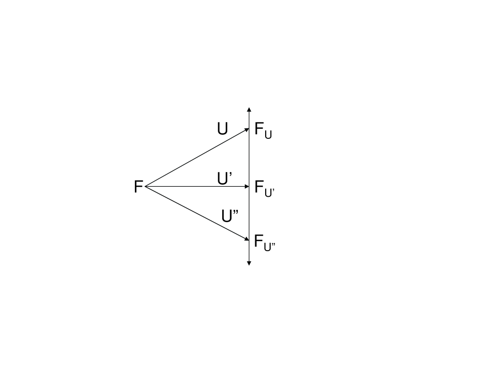
Figure 1: Relation between a Base Frame $F$ and Gauge Transformation Frames. A frame $F_{U}$ is associated with each gauge transformation $U$ of the rational string states in $F$. The three frame connections shown are illustrative of the infinitely many connections, shown by the two headed vertical arrow. Each $F_{U}$ is based on real and complex numbers $\mathcal{R}_{U},\mathcal{C}_{U}$ and a space time arena $\mathcal{R}^{4}_{U}$.

There is an asymmetric relation between the parent frame $F$ and the $F_{U}$ frames. An observer in $F$ can view the $F_{U}$ frames and see and describe their construction. He can see that for each $U,$ $\mathcal{R}_{U}$ and $\mathcal{C}_{U},$ as sets of Cauchy operators on rational string states, and $\mathcal{R}_{U}^{4}$ are the real and complex numbers and space time arena that are the basis of $F_{U}$.

An observer in $F_{U}$ has a different view. To him $\mathcal{R}_{U},\mathcal{C}_{U}$ are abstract sets just as $R$ and $C$ are abstract to an observer in $F$. The observer in $F_{U}$ cannot see $\mathcal{R}_{U}$ and $\mathcal{C}_{U}$ as Cauchy operators in an underlying frame. Similarly he views space time, $\mathcal{R}^{4}_{U},$ as a $4-$tuple of abstract real numbers. This limit on his vision occurs because the observation that $R_{U},C_{U}$ are sets of Cauchy operators is external to or outside of his frame. In this way his view of the real and complex numbers and space time is the same as that of an observer in $F$ about his own real and complex numbers and space time. In addition, the observer in $F_{U}$ cannot see the frame $F.$ This is a result of the abstract, external nature of $\mathcal{R}_{U},\mathcal{C}_{U},$ and $\mathcal{R}^{4}_{U}.$

Possibly the most important aspect of the frame relations shown in Fig. 1 is that the construction can be iterated. This is based on noting that the definitions of binary complex rational string states, the basic arithmetic relations $=_{A}$ and $\leq_{A}$ and operations $+_{A},\times_{A},-_{A},\div_{\ell,A}$, Cauchy conditions, and definitions of the Cauchy operators, all have their equivalent definitions in $F_{U}.$ Note that a rational string state $|\gamma s,\delta t\rangle_{U}$ in $F_{U}$ is not the same as either the state $|\gamma s,\delta,t\rangle$ or $U|\gamma s,\delta,t\rangle.$

This iteration is illustrated in Fig. 2 that shows two stages of the iteration as well as the base frame $F$ at stage $0$. At each stage only three of the infinite number of frames, one for each gauge $U$, coming from each parent are shown. One sees that each frame in stage $2$ has an infinite number of parents, one for each gauge U, and each frame in stage $1$ has an infinite number of children, one for each gauge $U$.

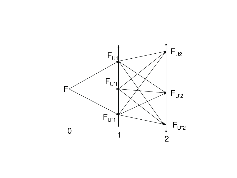
Figure 2: Three Iteration Stages of Frames coming from Frames. Only three frames of the infinitely many, one for each gauge $U,$ are shown at stages $1$ and $2$. The arrows connecting the frames show the iteration direction of frames emanating from frames.

It is also clear from the preceding that this iteration can be continued indefinitely to give stages $0,1,2,\cdots.$ Each stage $j$ contains an infinite number of frames $(F_{j})_{U}$, one for each gauge $U$. Each $(F_{j})_{U}$ has an infinite number of children, $(F_{j+1})_{U},$ one for each $U$, and an infinite number of parents, $(F_{j-1})_{U}$, also one for each gauge $U$. Also any frame $(F_{j})_{U}$ at any level $j$ can serve as the origin of a one way infinite directed structure of frames emanating from frames just as the frame $F$ does in Fig. 3.

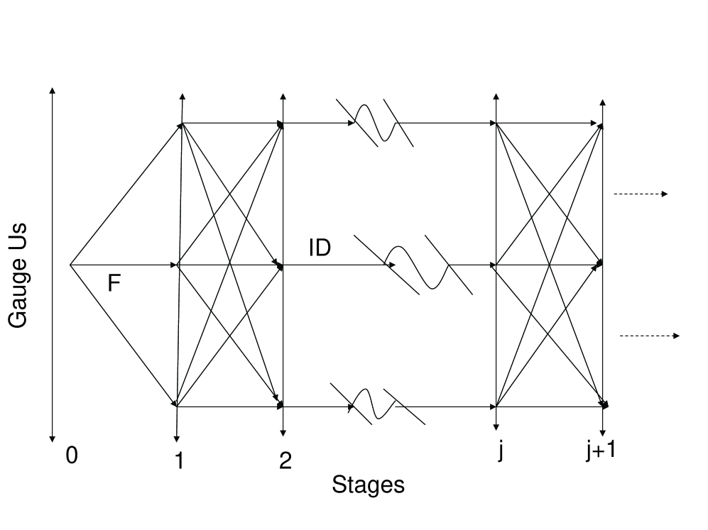
Figure 3: One way Infinite Iteration of Frames coming from Frames. Only three of the infinitely many frames, one for each gauge $U$ are shown for stages $1,2,\cdots,j,j+1,\cdots.$ The arrows connecting the frames show the iteration or emanation direction. The center arrows labeled ID denote iteration of the identity gauge transformation.

This figure also shows that iterated frame structure can be viewed as a field of frames on a two dimensional background of discrete stages in one direction and continuous gauge transformations in the other direction. Each point on each of the two headed arrows corresponds to a frame. The abcissa and ordinate denote respectively the discrete stages and the gauge transformations. The central arrows labeled ”ID” denote the identity gauge at each stage. Its location on the gauge axis depends on the arbitrary choice made in $F$ to represent the complex binary rational string states. Since an observer in $F$ can see all frames downstream he can determine which gauge at each stage is the identity.

One also notes that the whole structure shown in Fig. 3 can be translated to any frame. That is, any frame at any stage, can serve as the origin of a coordinate system just as $F$ does in the figure. In this case the arbitrary choice in the new frame of the gauge for the complex rational string states is the identity gauge for the new set up. In some ways this is similar to coordinate frame translations and rotations in usual 3D space.

The frame field in Fig. 3 has the problem that not all frames are equivalent. The base frame $F$ is unique or special in that for it $R$, $C$, and space time $R^{4}$, are external, or abstract and given. They are not sets of operators in any frame. These aspects of $F$ are outside the whole frame field of the figure and would have to be meaningful in some absolute sense, whatever that is.

One way to escape this problem is to extend the frame field to infinity in both stage directions. This is shown in Fig. 4 where stages are labeled with all integers. In this case there is no special frame as each frame has an infinite number of children and parents, one child and one parent for each gauge $U$. The frame field retains the basic direction of frames emanating from frames as expressed by the parent child relationship.

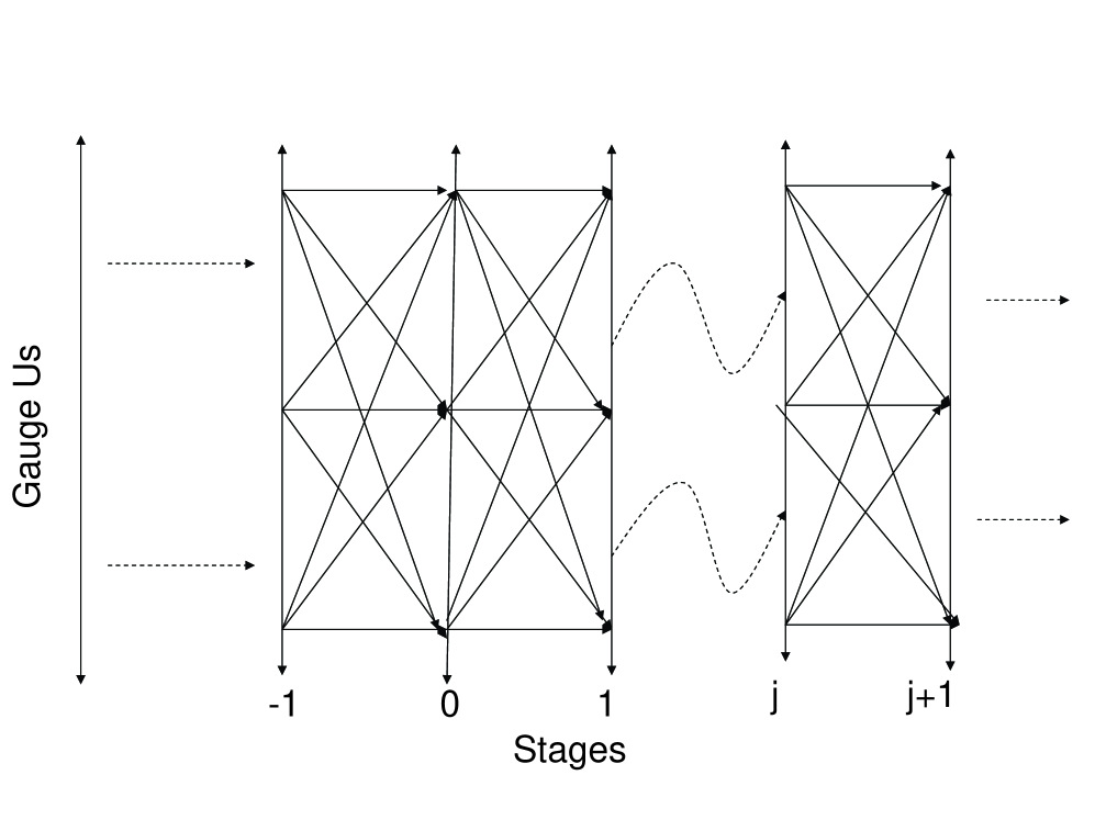
Figure 4: Two way Infinite Iteration of Frames coming from Frames. Only three of the infinitely many frames, one for each gauge $U$ are shown at each stage $\cdots,-1,0,1,\cdots,j,j+1,\cdots$. The solid arrows connecting the frames show the iteration or emanation direction. The wavy arrows denote iterations connecting stage $1$ frames to those at stage $j$. The straight dashed arrows denote infinite iterations from the left and to the right.of the identity gauge transformation.

This provides a satisfactory solution to the problem of the meaning of the existence of $R,C$, and $R^{4}$ in some absolute sense. For the two way infinite frame field there are no external or abstract $R,C,$ and $R^{4}.$ The frame field is background independent in that there is no space time or real or complex number fields that exist in an absolute sense.

Instead these exist in a relative sense only in that the real and complex number basis for each frame in the field are external and abstract for an observer in the frame. They are not external or abstract for an observer in any parent frame as they are consist of sets of Cauchy operators based on gauge transformations of complex rational string states in the parent frame. In this way the notion of idealized mathematical existence of real and complex numbers and of space time is relative as it is internal to the frame field. It has meaning only for observers within frames. This point will be taken up again in Section VII on the connection of the frame field to physics.

VI String Number Bases

VI.1 $k\geq 2$

So far, the treatment has been based on qubit strings. These correspond to binary representation of numbers. However, from a mathematical or physical point of view, there is nothing special about the base $2$. Any base $k$ with $k\geq 2$ is just as good as any other. Use of the base $2$ as the basis of computations may have computational advantages, but these do not seem to be relevant to physics in any basic sense.

It follows that the restriction to $k=2$ should be removed. The approach taken here to accomplish this is based on what might be called the maximum efficiency of representing all rational numbers as the set of all finite digit strings in a base $k$. Note that the representation of a real or imaginary rational number is by a single string state, not by pairs of string states.

The problem at hand is to determine the smallest base, $k_{min}$ for representing the rational number $1/n$ exactly as a finite base $k$ digit string. It is easy to convince oneself that if $n$ is a prime number, then $k_{min}=n.$ If $n=p_{1}^{h_{1}}p_{2}^{h_{2}}\cdots p_{m}^{h_{m}}$ is a product of $m$ primes to powers $h_{1}\cdots h_{m}$, then $k_{min}=p_{1}p_{2}\cdots p_{m}$ is the product of the $m$ primes all to the first power. It is sufficient to consider representations of $1/n$ because any base $k$ that can represent $1/n$ exactly can also represent $j/n$ exactly where $j$ is any integer. For $n=2,3,\cdots$ the corresponding pairs $(n,k_{min})$ are $(2,2),(3,3),(4,2),(5,5),(6,6)(7,7),(8,2),(9,3),(10,10)$, etc. One sees from this that the sequence of increasing minimal bases is given by $k_{min}=p_{1}\cdots p_{m}$ the product of the first $m$ primes for $m=2,3,5,\cdots.$

These aspects can be incorporated into the use of complex rational string states by expanding the qubit base to a qukit base where

$$k=p_{1}p_{2}\cdots p_{m}.$$ (45)

There are two options. One is to consider qukits as single systems with $k$ internal states. These would be represented here by AC operators $a^{{\dagger}}_{\alpha,j},a_{\alpha,j},b^{{\dagger}}_{\beta,j},b_{\beta,j}$ where $\alpha,\beta$ range over $k$ system states.

The other option, which will be used here, is to consider a base $k$ qukit where $k$ satisfies Eq. 45 as an $m$ tuple of qupits , $qu2it\times qu3it\cdots\times qu(p_{m})it,$ as a product of $m$ systems with the $j$ system type having $p_{j}$ internal states. These would be represented by $m$ different $a$ and $b$ operators $(a^{{\dagger}}_{1})_{\alpha_{1},j},(a^{{\dagger}}_{m})_{\alpha_{m},j},$ $(b^{{\dagger}}_{1})_{\beta_{1},j},\cdots,(b^{{\dagger}}_{m})_{\beta_{m},j}$ and similarly for the annihilation operators. Here $\alpha_{j},\beta_{j}$ refer to $p_{j}$ different states of the type $j$ system.

In this case the individual creation operators appearing in Eqs. 3 and 4 that define the complex rational string states $|\gamma s,\delta t\rangle$ are replaced by a product of the $m$ different types. That is, $a^{{\dagger}}_{s(j),j}$ and $b^{{\dagger}}_{t(j),j}$ are replaced by $\prod_{h=1}^{m}(a^{{\dagger}}_{h})_{s_{h}(j),j}$ and $\prod_{h=1}^{m}(b^{{\dagger}}_{h})_{t_{h}(j),j}$ in these equations. In this case a state $|\gamma s,\delta t\rangle$ is given by

$$|\gamma s,\delta t\rangle=c^{{\dagger}}_{\gamma,0}\prod_{j=l_{r}}^{u_{r}}\prod_{h=1}^{m}(a^{{\dagger}}_{h})_{s_{h}(j),j}d^{{\dagger}}_{\delta,0}\prod_{j=l_{i}}^{u_{i}}\prod_{h=1}^{m}(b^{{\dagger}}_{h})_{t_{h}(j),j}|0\rangle.$$ (46)

Here $s_{h}$ and $t_{h}$ are functions from their respective domains $[l_{r},u_{r}],[l_{i},u_{i}]$ to $\{0,1,\cdots,p_{h}-1\}.$ Alternatively this state could be represented as the product of the states of m $qup_{j}it$ strings, one for each $j=1,2,\cdots,m:$

$$|\gamma s,\delta t\rangle=\times_{h=1}^{m}[c^{{\dagger}}_{\gamma,0}\prod_{j=l_{r}}^{u_{r}}(a^{{\dagger}}_{h})_{s_{h}(j),j}d^{{\dagger}}_{\delta,0}\prod_{j=l_{i}}^{u_{i}}(b^{{\dagger}}_{h})_{t_{h}(j),j}|0\rangle].$$ (47)

Definitions of the arithmetic relations, $=_{A}$ and $\leq_{A},$ and operations $+_{A},\times_{A},$ $-_{A},\div_{A,\ell}$ are more complex but nothing new is involved. It is similar to changes needed in replacing single digits which can range from $0$ to $k-1$ to an $m$ tuple of digits where the $hth$ ranges from $0$ to $p_{h}-1.$ Similarly the definitions of the operators $\tilde{O}$ and their Cauchy convergence can be extended to apply here. In this case the nonnegative integer states $|\gamma s\rangle$ become $|\gamma s\rangle=c^{{\dagger}}_{+,0}\prod_{h=1}^{m}(a^{{\dagger}}_{h})^{s_{h}}_{[0,u_{r}]}|0\rangle$ with the Cauchy condition given by Eq. 23.

As was the case for $k=2$ these extended Cauchy operators can be collected into equivalence classes that are real and complex numbers $\mathcal{R}_{k},\mathcal{C}_{k}$. Also $\mathcal{R}_{k}^{4}$ can be used to represent space time. The resulting reference frames for different values of $k$ are all isomorphic to one another as $\mathcal{R}_{k}$ and $\mathcal{C}_{k}$ are isomorphic to $\mathcal{R}_{k^{\prime}}$ and $\mathcal{C}_{k^{\prime}}.$

Local and global gauge transformations are extended here from being elements of $SU(2)$ to elements of the direct product group $U(1)\times SU(2)\times SU(3)\times SU(5)\cdots\times SU(p_{m}).$ For each element $U=U_{1}\times U_{2}\cdots\times U_{m}$ of this group one can describe corresponding real and complex numbers and space time $R_{U},C_{U},$ and $R^{4}_{U}.$ The reason $U(1)$ is present will be discussed shortly. It is interesting to speculate that if the prime numbers correspond to the number of projections of spin systems then the group product above corresponds to spins $0,1/2,1,2,3,5,\cdots,(p_{m}-1)/2.$ All these systems are bosons except the spin $1/2$ systems which are fermions. Also the local gauge group $U(1)\times SU(2)\times SU(3)$ plays an important role in the standard model of physics Novaes ; Cottingham .

VI.2 $k=1$

Unary representations of numbers are not usually considered because the length of strings of one symbol needed to represent a number $n$ is proportional to $n$ instead of $\log{n}.$ Also all arithmetic operations are exponentially hard. However this representation should be included here because $1$ is a prime number and because it is present in an essential way.

It is of interest to note that base restrictions for expressing rational numbers, $1/n,$ as finite strings in different bases does not apply to integers. All integers can be expressed as finite strings in any base. It is tempting to ascribe this to the observations that $1$ is a prime factor of any integer and that integers seem to be the only type of number expressible in an unary representation.

The reason the unary representation is present in an essential way is that it is the only number representation that is extensive. Any finite collection of physical systems is itself an unary representation of a number, the number of objects in the collection. Also the magnitude of any extensive physical property of a system which changes in discrete steps is an unary representation of a number, the number of steps in the magnitude.

In the same sense a string of qubits is an unary representation of a number that is the number of qubits in the string. This is the case whatever states the qubit string is in, including complex rational string states. It follows that one should include global and local $U(1)$ gauge transformations. These correspond to transformations on the AC operators in Eq. 3 given by

$$\begin{array}[]{c}a^{{\dagger}}_{\alpha,j}\rightarrow U_{j}a^{{\dagger}}_{\alpha,j}=e^{i\theta_{j}}a^{{\dagger}}_{\alpha,j}\\ b^{{\dagger}}_{\beta,k}\rightarrow U_{k}b^{{\dagger}}_{\beta,k}=e^{i\phi_{k}b^{{\dagger}}_{\beta,k}}.\end{array}$$ (48)

If $\theta_{j}$ and $\phi_{k}$ are independent of $j$ and $k$ then $U$ is a global gauge transformation. Otherwise it is local.

VII Connection to Physics

VII.1 General Aspects

It is useful at this point to define a frame stage operator $W(U)$, parameterized by $U,$ that takes a frame $F_{U^{\prime}}$ at stage $j$ to a frame $F_{U^{\prime\prime}}$ at stage $j+1:$

$$F_{U^{\prime\prime}}=W(U)F_{U^{\prime}}$$ (49)

where $U^{\prime\prime}=UU^{\prime}.$ For any path $F_{U_{j}},F_{U_{j+1}},\cdots,F_{U_{j+h}}$ of frames from stage $j$ to stage $j+h$ there is an associated product of frame stage operators that relates the initial and final frames by

$$F_{U_{j+h}}=W(U^{\prime}_{j+h})W(U^{\prime}_{j+h-1})\cdots W(U^{\prime}_{j+1}F_{U_{j}}.$$ (50)

Here

$$U_{j+k}=U^{\prime}_{j+k}U_{j+k-1}$$ (51)

for $k=1,\cdots,h.$

It follows from the properties of frames in the frame field that $W(U)$ can be expressed as the product of an isomorphism $I$ and a gauge dependent operator $V(U)$ as $W(U)=V(U)I.$ Here $I=W(ID)$ is the stage step operator corresponding to the identity gauge and $V(U)$ changes a frame $F_{U^{\prime}}$ at any stage to a frame $F_{U^{\prime\prime}}$ at the same stage. Since all frames at any stage are unitarily equivalent, one sees that any pair of frames in the field are equivalent as far as physics is concerned. The physical descriptions and dynamics of systems on one frame is related to that in another frame by a product of isomorphisms $W(ID)$ and unitary equivalence maps $V(U).$ However this is quite different from saying the physics is the same in each frame.

This is in direct contradiction with our experience. Physically there is only one space time as $R^{4},$ and there is one set each of abstract real and complex numbers. The space time arena in which physics is done includes all of space time and it covers cosmological as well as Planck aspects. There is no multitude of space times and of real and complex numbers which are unitarily and isomorphically related.

The consequence of this is that there is an important ingredient left out of the treatment so far. This is that one must investigate various methods to make the physics in all frames the same, not just unitarily and isomorphically equivalent. If this can be achieved then all frames in the frame field describe the same physics which, hopefully, is the physics that is observed. Note that it is sufficient to show that any one frame can be identified with a parent frame. This is sufficient to collapse the frame field to one frame.

Details of how to achieve this must await future work. They may include quantum to classical limits by letting the qubits become increasingly complex, massive, and more classical, taking $m$ on $p_{m},$ the $mth$ prime, to infinity, and many other possibilities. One should also note that the existence of superselection rules corresponds to a reduction of frames as there are no frames connecting superselected subspaces of states Enk ; AharonovII .

Another point concerns experimental support for the frame picture shown here. This is especially relevant because our experience does not show in any direct way the existence of many frames. One possible way this might occur is for a physical prediction or theory to arise from the frame picture that has not been possible so far.

A speculative potential candidate is a new approach to the unification of gravity with quantum mechanics. This is based on the observation that the frame structure shown here allows a different approach to this problem and possibly to other problems. So far, attempts to solve this problem, such as string theory, correspond here to an observer in a frame $F$ trying to unite quantum mechanics with gravity for the space time and real, $R$, and complex, $C$, numbers of his own frame. One might expect problems with this since $R$, $C$, and the space time $R^{4}$ are abstract and given entities for $F.$ All properties they may have, that derive from their origin as operators on physical systems, are external to $F.$ They are available to an observer in a parent or ancestor frame but not to an observer in $F$.

This results in the possibility that some physical properties of Cauchy operators that are based on systems in rational string states in a parent frame could be interpreted by an observer in frame $F$ as the existence of gravity for his background space time. This avoids the situation of an observer having to tie gravity with quantum mechanics for his own space time. Also since every frame has parent and ancestor frames (Fig. 4) observers in all frames would report the existence of gravity in their physical universe. At this point, this idea remains to be verified. However, if it is successful, it would help to support the view presented here.

It also is worth noting that the two way infinite frame field, Fig. 4, shares a feature in common with loop quantum gravity Smolin ; Rovelli . This is that they are both space time background independent. Here he background independence is based on the observation that there is no fixed external space time background associated with the frame field. Space times are backgrounds only in a relative sense. Each frame has a space time that is a background to an observer in the frame. However there are as many space time backgrounds as there are frames in the frame field. No one is privileged over another. There is no space time background for the field itself.

VII.2 The Decoherent Free Subspace Approach

One approach to connecting the frame field to the one observed frame of physics is based on changing the definition of qubits in a way so the qubit states are invariant under a group of some gauge transformations. This has the result of collapsing all frames at any stage $j$ that are distinguished by any gauge $U$ in the group into one stage $j$ frame. If this could be extended to all gauge $U,$ then all stage $j$ frames could be collapsed into just one frame at $j$.

This idea is already in use in a slightly different context in the theory of decoherence subspaces (DFS) Lidar ; LidarII . The goal of the DFS method of constructing quantum error correction codes is to exhibit two subspaces of states of two or more physical qubits that are invariant under different types of errors. States in one subspace are the $0$ logical qubit states. States in the other are the $1$ logical qubit states.

This distinction between logical and physical qubits has not been made so far in that logical qubit states have been identified with states of physical systems as physical qubit states. In general, however, logical qubit states, correspond to projection operators $P_{0_{L}}P_{1_{L}}$ on two subspaces of states of two or more physical qubits. Any pure state of physical qubits in the $P_{0_{L}}$ or $P_{1_{L}}$ subspace corresponds respectively to a logical qubit state $|0\rangle_{L}$ or $|1\rangle_{L}$. Mixed states in the subspaces would be represented by density operators $\rho_{0_{L}},\rho_{1_{L}}.$

In this more general case the whole construction presented here of complex rational string states, real and complex numbers as Cauchy operators, and different frames $F_{U}$ with associated space times $\mathcal{R}^{4}_{U},$ would be expanded to describe rational string states in terms of strings of the logical qubit subspace projection operators. The advantage of this approach is that, logical qubit subspaces can be defined that are invariant under the action of global gauge $U$ acting on the physical qubit states.

The DFS approach Lidar ; LidarII to quantum error avoidance in quantum computations makes use of this generalization. In this approach quantum errors correspond to gauge transformations $U$, so the goal is to find subspaces of states that are invariant under at least some gauge $U$. One way to achieve this for qubits is based on irreducible representations of direct products of $SU(2)$ as the irreducible subspaces are invariant under the action of some $U$. Here, to keep things simple, the discussion is limited to binary rational string states $(k=2)$.

As an example, one can show that Enk the subspaces defined by the irreducible 4 dimensional representation of $SU(2)\times SU(2)$ are invariant under the action of any global $U$. The subspaces are the three dimensional subspace with isospin $I=1$, spanned by the states $|00\rangle,|11\rangle,1/\sqrt{2}(|01\rangle+|10\rangle)$ and the $I=0$ subspace containing $1/\sqrt{2}(|01\rangle-|10\rangle).$ States in these subspaces are logical qubit states. The action of any global $U$ on states in the $I=1$ subspace can change one of the $I_{z}$ states into linear superpositions of all states in the subspace. But it does not connect the states in the $I=1$ subspace with that in the $I=0$ subspace.

It follows that replacement of the physical qubit states in the complex rational string state by logical qubit states from the invariant subspaces, gives the result that, for all global $U$, the $F_{U}$ frames at any stage $j$ all become just one frame at stage $j$. The price for this frame reduction is the increased entanglement complexity of logical qubit states in a parent frame at stage $j-1.$

This process can be extended in several ways. One way is to consider logical qubits whose states are superpositions of states of $3$ physical qubits Enk ; Lidar . In this case the subspaces of interest are the $8$ dimensional irreducible subspaces of $SU(2)\times SU(2)\times SU(2)$. These correspond to one $I=3/2$ subspace and two $I=1/2$ subspaces of $3$ physical qubit states. In Enk ; Lidar the two $I=1/2$ subspaces are taken to be the logical qubit $0$ and $1$ subspaces.

VIII Summary and Discussion

In this work the basic importance of real and complex numbers to physics is emphasized. All physical theories are mathematical structures over the real and complex numbers, and space time is based on a 4 tuple of the real numbers. These aspects have been used to define fields of iterated quantum frames that are based on underlying complex rational string states and their gauge transformations. Rational string states are defined as products of AC operators acting on the vacuum string state. Sequences of these states are replaced by operators $\tilde{O}$ acting on the string states corresponding to nonnegative integers.

The Cauchy condition for sequences of these states is used to define Cauchy operators. (Equivalence classes of) These operators are real and complex numbers in the same sense as elements of $R$ and $C$ which are the basis of the Fock space in which the AC operators are defined. The sets $\mathcal{R},\mathcal{C}$ and $\mathcal{R}^{4}$ of Cauchy operators are the real and complex numbers and space time that are the basis of a stage $1$ frame $F_{1}$.

The frame base is greatly expanded by gauge transformations on the rational string states. For each gauge $U$ one has sets of Cauchy operators $\tilde{O}_{U}$ that correspond to real $\mathcal{R}_{U}$ and complex $\mathcal{C}_{U}$ numbers and space time $\mathcal{R}^{4}_{U}.$ These form the basis for an infinite number of stage $1$ frames $F_{U}$, one for each $U$ (Fig. 1). All these frames are equivalent as they are related by unitary transformations. $F_{1}=F_{ID}$ where $ID$ is the identity.

This process of frame construction can be iterated in one or two directions. This gives either one way infinite (Fig. 3) or two way infinite (Fig. 4) fields of frames coming from frames. For a one way infinite field, each frame has an infinite number of children frames, one for each $U$. For a two way infinite field, each frame has, in addition, an infinite number of parents, one for each $U$. The frame fields have an inherent direction built in that is represented by stage labels as integers.

Some properties of the frame fields are noted. Each frame includes all physical theories as mathematical structures over the real and complex numbers irrespective of their use of a space time arena to describe systems dynamics. All frames at any one stage are unitarily equivalent and any two frames at the same or different stages are isomorphic to each other.

The one way and two way infinite frame fields are different in that the base frame of a one way infinite field requires sets of real and complex numbers and a space time that is abstract and external in some absolute sense. They are not related to any frame. For the two way infinite frame field there are no external abstract real and complex numbers and no background space time. All real and complex numbers and space times are external and abstract in a relative sense only in that they are external and abstract relative to a frame. However they are internal objects as sets of Cauchy operators in a parent frame.

An important problem is to connect the field of frames to the one frame containing the observed physical universe. The goal of any process to achieve this is to identify as many frames as is possible with one frame. This is needed because it is not sufficient that frames in the frame field are isomorphic. They must become the same in some limit. It is noted that the method of decoherence free subspaces Lidar ; LidarII can be used to identify all frames in a stage that are related by global gauge transformations.

It is clear that much remains to be accomplished. However one has a very rich structure at hand with many possibilities to investigate. Also the structure enables a new approach to physical problems in that the dynamics of qukit systems in a frame $F$ is reflected in the dynamics of the Cauchy operators in $F$. It is possible that this would be seen in a frame $F_{U}$ as some type of effect on the space time of the frame. This suggests the possibility of a new way to approach the problem of combining gravity with quantum mechanics in that certain dynamics of quantum systems in $F$ appear in $F_{U}$ as the effect of gravity on physical systems. It is also possible that the approach of Ashtekar and collaborators Ashtekar ; AshtekarI ; AshtekarII to loop quantum gravity may be useful here.

Other avenues to investigate include the use of different number bases by expanding gauge transformations from those based on $SU(2)$ to those based on elements of $U(1)\times SU(2)\times\cdots\times SU(p_{m}).$ These are suitable for qukits where the base $k=p_{1}\cdots p_{m}.$ Here $p_{m}$ is the $mth$ prime number.

Other possible methods of frame identification include the possibility of turning the one and two infinite frame fields into cyclic frame fields by identifying two different stages. Also the possibility of using the least action principle in a Feynman path integral over the frame field needs to be examined.

In any case it is pleasing to note that this approach of constructing iterated frame fields corresponds to definite steps towards the much desired goal of constructing a coherent theory of physics and mathematics together BenTCTPM .

Finally it should be noted that the structure of frames emanating from frames has nothing to do with the Everett Wheeler view of multiple universes Everett . If these multiple universes exist, then they would exist within each frame in the field.

References

- (1) Y. Aharonov and T. Kaufherr, Phys. Rev. D 30, 368- (1984).
- (2) E. Bagan, M. Baig, and R. Mnoz-Tapia, Phys. Rev. Lett. 87, 167901, (2001).
- (3) T. Rudolph and L. Grover, Phys. Rev. Lett. 91, 217905, (2003).
- (4) S. D. Bartlett, T. Rudolph, and R. W. Spekkens, Phys. Rev. A 70, 032307 (2004).
- (5) S. J. van Enk, Phys. Rev. A 71, 032339 (2005).
- (6) S.J. van Enk, Arxiv preprint quant-ph/0602079.
- (7) Paul Benioff, Arxiv preprint quant-ph/0508219.
- (8) Yakir Aharonov and Leonard Susskind, Phys. Rev. 155,1428-1431, (1967)¿
- (9) Mark S. Byrd, Daniel Lidar, Lian-Ao Wu, and Paolo Zanardi, Phys. Rev A 71, 052301 (2005).
- (10) Paul Benioff, Found. Phys. 35, 1825-1856, (2005).
- (11) Lee Smolin, Arxiv preprint hep-th/0507235.
- (12) Carlo Rovelli, Arxiv preprint gr-qc/0604045; Quantum Gravity, Cambridge University Press, Cambridge, UK, (2004).
- (13) Gary Horowitz, ArXiv preprint gr-qc/0410049.
- (14) Paul Benioff, Phys. Rev. A 72, 032314 (2005).
- (15) M. Toller, Nuovo Cim. B112, 1013-1026, (1997), Arxiv preprint, gr-qc/9605052.
- (16) Gaisi Takeuti, Two Applications of Logic to Mathematics Kano Memorial Lecture 3, Princeton University Press, New Jersey, 1978.
- (17) Martin Davis, Internat. Jour. Theoret. Phys. 16,867-874,(1977).
- (18) E. I. Gordon, Soviet Math. Dokl. 18, 1481-1484 (1977).
- (19) G. L. Litvinov, V. P. Maslov, and G. B. Shpiz, Archives preprint, quant-ph/9904025, v5, 2002.
- (20) J. V. Corbett and T. Durt, Archives preprint, quant-ph/0211180 v1 2002.
- (21) K. Tokuo, Int. Jour. Theoretical Phys., 43, 2461-2481, 2004.
- (22) Jerzey Krol, ”A Model of Spacetime. The Role of Interpretations in Some Grothendieck Topoi”, preprint, (2006).
- (23) Y. Jack Ng and H. Van Dam, Int. Jour. Mod. Phys. A 20, 1328-1335 (2005).
- (24) Florian Girelli and Etera R. Levine Arxiv preprint gr-qc/0501075.
- (25) Damiel Terno, Arxiv preprint gr-qc/0512072.
- (26) Alejandro Perez, Arxiv preprints, gr-qc/0601095; gr-qc/0409061.
- (27) S. F. Novaes, Arxiv preprint hep-th/0001283.
- (28) A. N. Cottingham and D. A. Greenwood, An Introduction to the Standard Model of Physics, Cambridge University Press, Cambridge, UK, 1998.
- (29) J. Kempe, D. Bacon, D. A. Lidar, and K. B. Whaley, Phys. Rev. A 63, 042307 (2001).
- (30) Abhay Ashtekar, New Journal of Physics, 7, 198 (2005), Arxiv preprint, gr-qc/0410054.
- (31) Abhay Ashtekar, Arxiv preprint, gr-qc/99010123.
- (32) Abhay Ashtekar and Jerzy Lewandowski, Arxiv preprint, hep-th/9603083.
- (33) Hugh Everett III, Rev. Mod. Phys. 29, 454-462, (1957); John A. Wheeler, Rev. Mod. Phys. 29, 463-465 (1957).