3D phase-matching conditions for the generation of entangled triplets by $\chi^{(2)}$ interlinked interactions

Maria Bondani

National Laboratory for Ultrafast and Ultraintense Optical Science, Consiglio Nazionale delle Ricerche, Istituto Nazionale per la Fisica della Materia, UnitΓ  di Como, via Valleggio 11 - 22100 Como, Italy

maria.bondani@uninsubria.it

Alessia Allevi, Eleonora Gevinti, Andrea Agliati, Alessandra Andreoni

Dipartimento di Fisica e Matematica, UniversitΓ  degli Studi dell’Insubria and Istituto Nazionale per la Fisica della Materia, UnitΓ  di Como, via Valleggio, 11 - 22100 Como, Italy

Abstract

An analytical calculation of the interaction geometry of two interlinked second-order nonlinear processes fulfilling phase-matching conditions is presented. The method is developed for type-I uniaxial crystals and gives the positions on a screen beyond the crystal of the entangled triplets generated by the interactions. The analytical results are compared to experiments realized in the macroscopic regime. Preliminary tests to identify the triplets are also performed based on intensity correlations.

OCIS codes: (190.4410) Nonlinear optics, parametric processes; (270.0270) Quantum optics.

References and links

  • [1] A. Ferraro, M. G. A. Paris, M. Bondani, A. Allevi, E. Puddu, and A. Andreoni, β€œGeneration and applications of continuous variable three-mode entanglement in $\chi^{(2)}$ optical media,” J. Opt. Soc. Am. B 21, 1241-1249 (2004).
  • [2] A. V. Rodionov and A. S. Chirkin, β€œEntangled photon states in consecutive nonlinear optical interactions,” JETP Lett. 79, 253-256 (2004).
  • [3] A. S. Bradley, M. K. Olsen, O. Pfister, and R. C. Pooser, β€œBright tripartite entanglement in triply concurrent parametric oscillation,” Phys. Rev. A 72, 053805 (2005).
  • [4] P. van Loock and S. L. Braunstein, β€œMultipartite entanglement for continuous variables: a quantum teleportation network,” Phys. Rev. Lett. 84, 3482-3485 (2000).
  • [5] J. Jing, J. Zhang, Y. Yan, F. Zhao, C. Xie, and K. Peng, β€œExperimental demonstration of tripartite entanglement and controlled dense coding for continuous variables,” Phys. Rev. Lett. 90, 167903 (2003).
  • [6] T. Aoki, N. Takey, H. Yonezawa, K. Wakui, T. Hiraoka, A. Furusawa, and P. van Loock, β€œExperimental creation of a fully inseparable tripartite continuous-variable state,” Phys. Rev. Lett. 91, 080404 (2003).
  • [7] O. GlΓΆckl, S. Lorenz, C. Marquardt, J. Heersink, M. Brownnutt, C. Silberhorn, Q. Pan, P. van Loock, N. Korolkova, and G. Leuchs, β€œExperiment towards continuous-variable entanglement swapping: Highly correlated four-partite quantum state,” Phys. Rev. A 68, 012319 (2003).
  • [8] S. L. Braunstein and A. K. Pati, Quantum Information with Continuous Variables (Kluwer Academic, Dordrecht, 2003).
  • [9] S. L. Braunstein and P. van Loock, β€œQuantum information with continuous variables,” Rev. Mod. Phys. 77, 513-577 (2005).
  • [10] Chao-Kuei Lee, Jing-Yuan Zhang, J. Huang, and Ci-Ling Pan, β€œGeneration of femtosecond laser pulses tunable from 380 nm to 465 nm via cascaded nonlinear optical mixing in a noncollinear optical parametric amplifier with a type-I phase matched BBO crystal,” Opt. Express 11, 1702-1708 (2003). http://www.opticsexpress.org/abstract.cfm?id=73362
  • [11] M. Bondani, A. Allevi, A. Andreoni, E. Puddu, A. Ferraro, and M. G. A. Paris, β€œProperties of two interlinked interactions in non-collinear phase-matching”, Opt. Letters 29, 180-182 (2004), and erratum Opt. Letters 29, 1417–1417 (2004).
  • [12] M. G. A. Paris, A. Allevi, M. Bondani, and A. Andreoni are preparing a manuscript to be called β€œQuantum and classical correlations in tripartite states of light”.

1 Introduction

The production of multipartite entangled states by means of multiple nonlinear interactions occurring in a single nonlinear crystal has been recently suggested [1, 2, 3] as an alternative to the use of single-mode squeezed states [4, 5, 6] or of two-mode entangled states and linear optical elements [7]. As in the case of bipartite states produced by spontaneous parametric downconversion, such multipartite states display entanglement also in the macroscopic regime in which bright outputs are generated: for this reason they are particularly interesting for all the applications of continuous-variable entanglement [8, 9].
The possibility of realizing the simultaneous phase-matching (PM) of two traveling-wave parametric processes in a single crystal in a seeded configuration has been already demonstrated [10, 11]. In this paper we present the experimental realization of the same interlinked interactions starting from vacuum fluctuations. The output of the nonlinear crystal displays the entire ensemble of inseparable tripartite entangled states satisfying the PM conditions. In order to identify a triplet, we develop a 3D calculation of the characteristics of interlinked PM that reproduce the experimental phenomenology. Finally we perform a preliminary verification of the number of photons conservation law by means of intensity correlations.

2 Theory

We consider the Hamiltonian describing the simultaneous PM of a downconversion and an upconversion processes

Hint=Ξ³1​a1†​a3†+Ξ³2​a2†​a3+h.c.,formulae-sequencesubscript𝐻intsubscript𝛾1superscriptsubscriptπ‘Ž1†subscriptsuperscriptπ‘Žβ€ 3subscript𝛾2superscriptsubscriptπ‘Ž2†subscriptπ‘Ž3β„Žπ‘H_{\mathrm{int}}=\gamma_{1}a_{1}^{\dagger}a^{{\dagger}}_{3}+\gamma_{2}a_{2}^{{\dagger}}a_{3}+h.c.\;, (1)

where $\gamma_{1}\propto a_{4}$ and $\gamma_{2}\propto a_{5}$ are coupling coefficients. The two interlinked interactions involve five fields $a_{\mathrm{j}}$, two of which, say $a_{4}$ and $a_{5}$, enter the crystal and act as non-evolving pumps. When acting on the vacuum as the initial state, $H_{\mathrm{int}}$ admits the following conservation law

$$N_{1}(t)=N_{2}(t)+N_{3}(t)\;,$$ (2)

being Nj​(t)=⟨aj†​(t)​aj​(t)⟩subscript𝑁j𝑑delimited-⟨⟩subscriptsuperscriptπ‘Žβ€ j𝑑subscriptπ‘Žj𝑑N_{\mathrm{j}}(t)=\langle a^{\dagger}_{\mathrm{j}}(t)a_{\mathrm{j}}(t)\rangle the mean number of photons in the j-th mode, and yields a fully inseparable tripartite state [1]. We consider the realization of Eq.Β (1) in a negative uniaxial crystal in type-I non-collinear PM interaction geometry. The processes must satisfy energy-matching ($\omega_{4}=\omega_{1}+\omega_{3}$, $\omega_{2}=\omega_{3}+\omega_{5}$) and PM conditions (${\mathbf{k}^{e}_{4}}={\mathbf{k}^{o}_{1}}+{\mathbf{k}^{o}_{3}}$, ${\mathbf{k}^{e}_{2}}={\mathbf{k}^{o}_{3}}+{\mathbf{k}^{o}_{5}}$), where $\omega_{\mathrm{j}}$ are the angular frequencies, ${\mathbf{k}_{\mathrm{j}}}$ are the wavevectors and o,e indicate ordinary and extraordinary field polarizations. In order to investigate the geometrical constraints imposed by the PM conditions, we analytically calculate the output angles of each interacting field.

Refer to caption
Fig. 1: Scheme of the phase-matched interlinked interactions: $(x,y)$-plane coinciding with the crystal entrance face; $\alpha$, tuning angle; $\beta_{\mathrm{j}}$’s, angles to $(y,z)$-plane; $\vartheta_{\mathrm{j}}$’s, angles on the $(y,z)$-plane; $\varphi$, angle to the optical axis (OA).

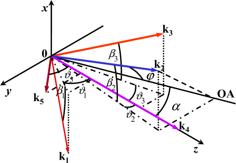
To simplify calculations, we assume, in the reference frame depicted in Fig.Β 1, that the two pumps lie in the $(y,z)$-plane containing the optical axis (OA) and the normal to the crystal entrance face and that the pump field $a_{4}$ propagates along the normal, $z$. The solutions corresponding to the effective experimental orientation of the crystal can be obtained by simply calculating the refraction of the beams at the crystal entrance/output faces. Accordingly, the PM conditions for the two interactions simultaneously phase-matched can be written as

$\displaystyle k_{1}\sin\beta_{1}+k_{3}\sin\beta_{3}$ $\displaystyle=$ $\displaystyle 0$ (3)
$\displaystyle k_{1}\cos\beta_{1}\sin\vartheta_{1}+k_{3}\cos\beta_{3}\sin\vartheta_{3}$ $\displaystyle=$ $\displaystyle 0$ (4)
$\displaystyle k_{1}\cos\beta_{1}\cos\vartheta_{1}+k_{3}\cos\beta_{3}\cos\vartheta_{3}$ $\displaystyle=$ $\displaystyle k_{4}$ (5)
$\displaystyle k_{2}\sin\beta_{2}$ $\displaystyle=$ $\displaystyle k_{3}\sin\beta_{3}$ (6)
$\displaystyle k_{2}\cos\beta_{2}\sin\vartheta_{2}$ $\displaystyle=$ $\displaystyle k_{3}\cos\beta_{3}\sin\vartheta_{3}+k_{5}\sin\vartheta_{5}$ (7)
$\displaystyle k_{2}\cos\beta_{2}\cos\vartheta_{2}$ $\displaystyle=$ $\displaystyle k_{3}\cos\beta_{3}\cos\vartheta_{3}+k_{5}\cos\vartheta_{5}$ (8)

where the angles are defined as in Fig.Β 1. The wavevectors $k_{\mathrm{j}}$ are defined as $k_{\mathrm{j}}=n_{\mathrm{j}}(\omega_{\mathrm{j}},{\mathbf{\hat{k}_{j}}})\omega_{\mathrm{j}}/c$, being $c$ the speed of light in the vacuum and $n_{\mathrm{j}}(\omega_{\mathrm{j}},{\mathbf{\hat{k}_{j}}})$ the refraction indices of the medium

$\displaystyle n_{j}\left(\omega_{j}\right)=n_{o}\left(\omega_{j}\right)$ $\displaystyle\quad j=1,3,5$ (9)
$\displaystyle n_{2}\left(\omega_{2},\varphi\right)=\left[\frac{\cos^{2}\varphi}{n_{o}^{2}(\omega_{2})}+\frac{\sin^{2}\varphi}{n_{e}^{2}(\omega_{2})}\right]^{-1/2}$ ; $\displaystyle n_{4}\left(\omega_{4},\alpha\right)=\left[\frac{\cos^{2}\alpha}{n_{o}^{2}(\omega_{4})}+\frac{\sin^{2}\alpha}{n_{e}^{2}(\omega_{4})}\right]^{-1/2}\;.$ (10)

where $n_{o,e}(\omega)$ are given by the dispersion relations of the medium. Note that $\cos\varphi=\cos\beta_{2}\cos(\vartheta_{2}-\alpha)$ and $\beta_{5}=\beta_{4}=\vartheta_{4}=0$.

For fixed frequencies and propagation directions of the pump fields, we are left with 11 variables ($\omega_{1}$, $\omega_{2}$, $\omega_{3}$, $\vartheta_{1}$, $\vartheta_{2}$, $\vartheta_{3}$, $\vartheta_{5}$, $\beta_{1}$, $\beta_{2}$, $\beta_{3}$, $\alpha$) and 8 equations only (energy conservation and Eqs.Β (3) to (8)). The problem can thus be solved by choosing three of the variables (say $\omega_{1}$, $\vartheta_{5}$ and $\alpha$) as parameters. The Appendix contains the algebraic procedure to analytically solve the problem. In order to efficiently handle the dependence of the solutions on the free parameters, we implemented the calculation by using the software Mathematica (Wolfram Research, IL).
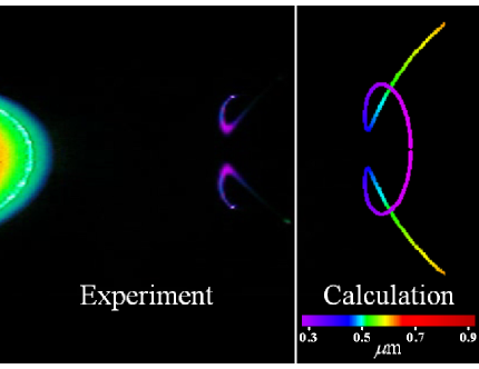
Refer to caption
Fig. 2: (1.271 MB) Movie showing the variation of the measured and calculated outputs of the crystal as a function of the tuning angle $\alpha$ for fixed external angle between the pumps. Left panel: picture of the output of the crystal taken with a commercial digital photocamera (no color correction applied). LHS: a portion of the downconversion cones. RHS: output of the upconversion process. Right panel: calculated output of the upconversion process.

In Fig.Β 2 we show one picture of the movie containing the comparison between measured and calculated results for the output of the crystal as a function of the tuning angle $\alpha$ for a fixed value of the external angle between the two pumps. Note that not all the calculated output frequencies appear in the experimental part due to the sensitivity of the camera sensor. As the pictures of the experimental outputs were taken on a screen located beyond the crystal normally to the direction of pump $a_{4}$, the calculations had to take into account both the rotation of the crystal and the refraction of the beams at the entrance and exit faces of the crystal. In particular, refraction at the exit face gives: $\sin\beta_{\mathrm{j,out}}=n_{\mathrm{j}}\sin\beta_{\mathrm{j}}$ and $\sin\vartheta_{\mathrm{j,out}}=n_{\mathrm{j}}/(1-n_{\mathrm{j}}^{2}\sin^{2}\beta_{\mathrm{j}})^{1/2}\cos\beta_{\mathrm{j}}\sin\vartheta_{\mathrm{j}}$.

3 Experiment

For the realization of the interaction described by Eq.Β (1), the pump fields were provided by the third-harmonics and the fundamental outputs of a continuous-wave mode-locked Nd:YLF laser regeneratively amplified at the repetition rate of 500 Hz (High Q Laser Production, Austria). In particular, the third-harmonic field ($\lambda_{4}=349$ nm, $\sim 4.45$ ps pulse duration) was used as the $a_{4}$ field producing the downconversion cones and the fundamental field ($\lambda_{5}=1047$ nm, $\sim 7.7$ ps pulse duration) as the $a_{5}$ field pumping the upconversion process.
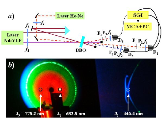
Refer to caption
Fig. 3: Upper panel: scheme of the experimental setup. BBO, nonlinear crystal; F1-3, filters; P1-3, pin-holes; $f_{1-5,\mathrm{s}}$, lenses; D1-3, p-i-n photodiodes; SGI, synchronous gated-integrator; MCA+PC, computer integrated multichannel analyzer. Lower panel: picture of the visible portion of the output states on a screen located beyond the nonlinear crystal.

As depicted in Fig.Β 3 $a$), both pumps were focused and injected into a $\beta$-BaB2O4 crystal (BBO, Fujian Castech Crystals, China, 10 mm $\times$ 10 mm cross section, 4 mm thickness) cut for type-I interaction ($\vartheta_{\mathrm{cut}}=34$ deg) at the angle $\vartheta_{5,\mathrm{ext}}=-34.8$ deg with respect to each other. The required superposition of the two pumps in time was obtained with a variable delay line. For alignment purposes, we used the light emitted by a He-Ne continuous-wave laser (Melles-Griot, CA, 5 mW max output power) to seed the process at $\lambda_{1}=632.8$ nm. The beam was collimated and sent to the BBO in the plane containing the pumps at the external angle $\vartheta_{1,\mathrm{ext}}=-2.54$ deg with respect to $a_{4}$. The seeded interactions produced two new fields: $a_{3}$ ($\lambda_{3}=778.2$ nm, $\vartheta_{3,\mathrm{ext}}=3.35$ deg) generated as the difference-frequency of $a_{4}$ and $a_{1}$, and $a_{2}$ ($\lambda_{2}=446.4$ nm, $\vartheta_{2,\mathrm{ext}}=-12.78$ deg) generated as the sum-frequency of $a_{3}$ and $a_{5}$. The pump fields were sufficiently intense so as to observe the process starting from vacuum fluctuations: as shown in the picture in Fig.Β 3 $b$), on a white screen located beyond the crystal it was possible to see both the tunable bright downconversion cones and the two polychromatic half-moons-shaped states generated by the upconversion process together with the spots of the fields generated by the seeded interactions.

The conservation law in Eq.Β (2) implies strong intensity correlations among the generated fields which are necessary but not sufficient to demonstrate the entangled nature of the triplet. We realized intensity-correlation measurements by filtering each portion of light in frequency and aligning three pin-holes of suitable diameters on the spots of the seeded process. Note that the seeding He-Ne light was switched-off once completed the alignment. The light selected by the pin-holes was focused on three p-i-n photodiodes (two, D1,2 in Fig.Β 3 $a$), S5973-02 and one, D3, S3883, Hamamatsu, Japan). The overall detection efficiencies in the three detection arms were $\eta_{1}=0.44$, $\eta_{2}=0.72$ and $\eta_{3}=0.43$. Each current output was integrated by a synchronous gated-integrator (SGI in Fig.Β 3 $a$)) in external trigger modality, digitized by a 13-bit converter (SR250, Stanford Research Systems, CA) and recorded in a PC-based multichannel analyzer. Data acquisition and analysis were performed with software LabView (National Instruments, TX). We evaluated the following correlation function on subsequent laser shots (k)

$$\Gamma(\mathrm{k})=\frac{\langle\left[m_{1}(\mathrm{i})-\langle m_{1}\rangle\right]\left[m_{2}(\mathrm{i}+\mathrm{k})+m_{3}(\mathrm{i}+\mathrm{k})-\langle m_{2}+m_{3}\rangle\right]\rangle}{\sigma(m_{1})\sigma(m_{2}+m_{3})}\,.$$ (11)

in which $m_{\mathrm{j}}$ is the number of detected photons and $\sigma(x)=(\langle x^{2}\rangle-\langle x\rangle^{2})^{1/2}$ is the standard deviation. It can be demonstrated [12] that in the case of bright triplets the correlation coefficient $\varepsilon\equiv\Gamma(0)$ must approach unity. The mean values of the detected photons in the three parties of the triplet were $M_{1}=1.082\times 10^{8}$, $M_{2}=2.3\times 10^{6}$ and $M_{3}=1.115\times 10^{8}$ and the measured correlation coefficient was $\varepsilon=0.916$.

4 Conclusions

The perfect agreement between calculations and experimental results demonstrates the correctness of the developed model. This enables us to forecast different interaction schemes that in the future will allow to overcome the experimental difficulties experienced in the present setup. In fact, the reason why the measured correlation coefficient is less than unity could be the imperfect selection of the triplet and/or the presence of spurious light in the same location.

Acknowledgements

This work was supported by the Italian Ministry for University Research through the FIRB Project n. RBAU014CLC-002. The Authors thank M.G.A. Paris (UniversitΓ  degli Studi, Milano) for theoretical support on correlations.

Present addresses: E. Gevinti, STMicroelectronics, via Olivetti, 2 - 20041 Agrate Brianza (MI), Italy; A. Agliati, Quanta System, via IV Novembre, 116 - 21058 Solbiate Olona (VA), Italy.

Appendix

We describe the analytical procedure to solve the equation system (3)-(8).

From the first of Eqs.Β (10) we write

$\displaystyle k_{2}=\left[G_{2}\cos^{2}\left(\vartheta_{2}-\alpha\right)\cos^{2}\beta_{2}+L_{2}\right]^{-1/2}\;,$ (12)

where $G_{2}=c^{2}/\omega_{2}^{2}\left[1/n_{o}^{2}(\omega_{2})-1/n_{e}^{2}(\omega_{2})\right]=1/k_{2,o}^{2}-1/k_{2,e}^{2}$ and $L_{2}=c^{2}/\omega_{2}^{2}1/n_{e}^{2}(\omega_{2})=1/k_{2,e}^{2}$. By squaring and summing Eqs.Β (3), (4) and (5) and defining $A=(k_{4}^{2}+k_{3}^{2}-k_{1}^{2})/(2k_{3}k_{4})$, we easily get

$\displaystyle\cos\beta_{3}=\frac{A}{\cos\vartheta_{3}}\;,$ (13)

whereas by squaring and summing Eqs.Β (6), (7) and (8) and Eqs.Β (7) and (8) we get

$\displaystyle k_{2}^{2}$ $\displaystyle=$ $\displaystyle k_{3}^{2}+k_{5}^{2}+2k_{3}k_{5}\cos\beta_{3}\left(\sin\beta_{3}\sin\vartheta_{5}+\cos\beta_{3}\cos\vartheta_{5}\right)$ (14)
$\displaystyle k_{2}^{2}\cos^{2}\beta_{2}$ $\displaystyle=$ $\displaystyle k_{3}^{2}\cos^{2}\beta_{3}+k_{5}^{2}+2k_{3}k_{5}\cos\beta_{3}\left(\sin\beta_{3}\sin\vartheta_{5}+\cos\beta_{3}\cos\vartheta_{5}\right)\;.$ (15)

By eliminating $k_{2}$ from Eqs.Β (14) and (15) and using Eq.Β (13) we find

$\displaystyle\cos^{2}\beta_{2}=\frac{k_{3}^{2}A^{2}\tan^{2}\vartheta_{3}+k_{5}^{2}+2k_{3}k_{5}A\left(\tan\vartheta_{3}\sin\vartheta_{5}+\cos\vartheta_{5}\right)}{k_{3}^{2}+k_{5}^{2}+2k_{3}k_{5}A\left(\tan\vartheta_{3}\sin\vartheta_{5}+\cos\vartheta_{5}\right)}\;.$ (16)

From Eq.Β (3) we obtain

$\displaystyle\sin\beta_{1}=-\frac{k_{3}}{k_{1}}\sin\beta_{3}\;.$ (17)

that, once substituted into Eq.Β (4) together with Eq.Β (13), gives

$\displaystyle\sin\vartheta_{1}=-\frac{k_{3}A}{\sqrt{k_{1}^{2}-k_{3}^{2}\sin^{2}\beta_{3}}}\;.$ (18)

We now divide Eq.Β (7) by Eq.Β (8) and use Eq.Β (13)

$\displaystyle\tan\vartheta_{2}=\frac{k_{3}A\tan\vartheta_{3}+k_{5}\sin\vartheta_{5}}{k_{3}A+k_{5}\cos\vartheta_{5}}\;.$ (19)

By squaring Eq.Β (12) and inserting Eq.Β (14) and Eq.Β (16) into it we get

$\displaystyle\cos^{2}\left(\vartheta_{2}-\alpha\right)=\frac{1-L_{2}\left[k_{3}^{2}+k_{5}^{2}+2k_{3}k_{5}\cos\beta_{3}\left(\sin\beta_{3}\sin\vartheta_{5}+\cos\beta_{3}\cos\vartheta_{5}\right)\right]}{G_{2}\left[k_{3}^{2}\cos^{2}\beta_{3}+k_{5}^{2}+2k_{3}k_{5}\cos\beta_{3}\left(\sin\beta_{3}\sin\vartheta_{5}+\cos\beta_{3}\cos\vartheta_{5}\right)\right]}\;.$ (20)

By substituting Eq.Β (13) into Eq.Β (20), expanding $\cos^{2}\left(\vartheta_{2}-\alpha\right)$ in Eq.Β (20) and using Eq.Β (19) to eliminate $\vartheta_{2}$, after some simplifications we get a quadratic algebraic equation for the variable $\tan\vartheta_{3}$

$\displaystyle a\tan^{2}\vartheta_{3}+b\tan\vartheta_{3}+c=0\;,$ (21)

whose coefficients are

$\displaystyle a$ $\displaystyle=$ $\displaystyle G_{2}A^{2}k_{3}^{2}\sin^{2}\alpha$
$\displaystyle b$ $\displaystyle=$ $\displaystyle 2G_{2}A\ k_{3}(A\ k_{3}+k_{5}\cos\vartheta_{5})\sin\alpha\cos\alpha+2G_{2}A\ k_{3}k_{5}\sin\vartheta_{5}\sin^{2}\alpha+2L_{2}A\ k_{3}k_{5}\sin\vartheta_{5}$
$\displaystyle c$ $\displaystyle=$ $\displaystyle G_{2}(A\ k_{3}+k_{5}\cos\vartheta_{5})^{2}(\cos^{2}\alpha-\sin^{2}\alpha)+2G_{2}k_{5}\sin\vartheta_{5}(A\ k_{3}+k_{5}\cos\vartheta_{5})\sin\alpha\cos\alpha$
$\displaystyle+$ $\displaystyle G_{2}(A^{2}k_{3}^{2}+k_{5}^{2}+2A\ k_{3}k_{5}\cos\vartheta_{5})\sin^{2}\alpha+L_{2}(k_{3}^{2}+k_{5}^{2}+2A\ k_{3}k_{5}\cos\vartheta_{5})-1\;.$

Once solved Eq.Β (21), we find $\vartheta_{3}$ and then all the other variables as a function of the free parameters $\omega_{1}$, $\alpha$ and $\vartheta_{5}$.