Quantum homodyne tomography of a two-photon Fock state

Abstract

We present a continuous-variable experimental analysis of a two-photon Fock state of free-propagating light. This state is obtained from a pulsed non-degenerate parametric amplifier, which produces two intensity-correlated twin beams. Counting two photons in one beam projects the other beam in the desired two-photon Fock state, which is analyzed by using a pulsed homodyne detection. The Wigner function of the measured state is clearly negative. We developed a detailed analytic model which allows a fast and efficient analysis of the experimental results.

Quantum properties of light beams can be described in terms of amplitude and phase or, in Cartesian coordinates, in terms of the “quadrature components” of the quantized electric field, associated with non-commuting operators $\hat{x}$ and $\hat{p}$. The corresponding observables, often called “quantum continuous variables”, are analogous to the position and the momentum of a particle, and from Heisenberg’s inequalities they cannot be determined simultaneously with an infinite precision. As a consequence, one cannot define a proper phase-space distribution $\Pi(x,p)$ for the electric field, but rather a quasidistribution $W(x,p)$ called the Wigner function. This function can be reconstructed by quantum homodyne tomography Vogel and Risken (1989), which consists in measuring several quadratures $\hat{x}_{\theta}=\hat{x}\;\cos\theta+\hat{p}\;\sin\theta$ with a homodyne detection, and applying an inverse Radon transform.

The most conspicuous property of the Wigner function is that it may take negative values for specific quantum states, as a signature of their non-classical nature. This is the case for Fock states, which contain a well-defined number of photons. Such states can be generated by using “twin” beams, which are produced by optical parametric amplification, and which contain perfectly correlated numbers of photons. Counting $n$ photons in one mode projects the other mode in a $n$-photon Fock state, which can then be analyzed using homodyne tomography. This was recently demonstrated for $n=1$ Lvovsky et al. (2001); Zavatta et al. (2004). However, up to now this method could not be applied for higher photon numbers, since the probability to generate simultaneously more than one photon pair was extremely low.

In this Letter we present a detailed analysis of a free-propagating light pulse prepared in a two-photon Fock state $(n=2)$. The measured Wigner function presents a complex structure and takes negative values. In addition to standard methods, we will also present a novel analytic model of the experiment, allowing an in-depth physical interpretation of the experimental results.

Figure 1: Experimental setup, and Wigner function of the two-photon state propagating in the experiment (corrected for homodyne detection losses, see text).

Our experimental setup is presented on Fig. 1. A pulsed Ti-Sapphire laser produces 180-femtosecond nearly Fourier-limited pulses with an energy of 40 nJ and a 800 kHz repetition rate Wenger et al. (2004). The high pulse peak power allows us to increase the pair production rate beyond what was available previously Lvovsky et al. (2001); Zavatta et al. (2004). The 850  nm pulses are frequency-doubled [second harmonic generation (SHG)] by a single pass in a $100\;\mu m$ thick non-critically phase-matched potassium niobate (KNbO₃) crystal. The frequency-doubled beam pumps an identical crystal used as an optical parametric amplifier (OPA), generating a two-mode squeezed state Wenger et al. (2005). To align the setup, a probe beam is injected in the OPA with an angle of $5^{\circ}$ to the pump direction. It allows to measure a classical phase-independent gain $g=1.07$. The homodyne detection is aligned on the idler beam, whereas the signal beam, after spatial and spectral filtering, is split between two avalanche photodiodes (APD) operating in a photon-counting regime. The detection of a coincidence by the APDs means that at least two photon pairs were created in the OPA by the same pulse. Since the gain $g$ is still relatively low the probability to create more than two pairs is small in this case. Therefore, a coincidence detected by the APDs conditionally prepares a two-photon state in the idler beam. Single-photon states are conditioned by single APD events. The prepared states are analyzed by a homodyne detection operating in a time-resolved regime. It samples each individual pulse, measuring one quadrature $X_{\theta}$ in phase with the local oscillator.

In previous $n=1$ state reconstruction experiments Lvovsky et al. (2001); Zavatta et al. (2004); Bertet et al. (2002), it was generally admitted that the generated states are phase-independent. In our case, the production rate of single photons is very high, and we can record the full $n=1$ quadrature distribution in less than a second, during which phase drifts are negligible. Therefore we did check experimentally that both the unconditional (thermal) and singly-conditional $(n=1)$ probability distributions do not depend on $\theta$. Then it is quite reasonable to assume that this is also the case for the $n=2$ state, as it was done for the $n=1$ state in older experiments.

In a 2-hour experimental run we acquired $105.000$ homodyne data points conditioned on two-photon coincidences (40 seconds were enough to acquire 180.000 single-photon events). Dividing the data into 64-bin histograms, we obtained the quadrature distributions presented on Fig. 2. With a numerical Radon transform, we reconstructed the Wigner functions associated with the measured states (see Fig. 3), both clearly negative. Their minima and their values at the origin are presented in Table 1. To determine the Wigner functions of the generated states, presented on Fig. 4, we correct for the homodyne detection losses by using a standard maximal-likelihood (MaxLik) algorithm Fiurášek and Hradil (2001); Lvovsky (2004), taking into account an independently measured homodyne efficiency $\eta=80\%$.

Figure 2: Experimental quadrature measurements, and quadratures reconstructed using our model (see text)

Figure 3: Wigner functions of the measured uncorrected states, reconstructed by a standard Radon transform, compared to those obtained using the model described in the text

Table 1: Critical values of the Wigner functions corresponding to the measured uncorrected data (Raw, obtained from the Radon transform), to the state corrected for homodyne detection losses (Corrected, obtained from the MaxLik method) and to the ideal state (Ideal).

	2 photons			1 photon
	$min(W_{2})$	$W_{2}(0)$		$min(W_{1})=W_{1}(0)$
Raw	$-0.009\pm 0.003$	$0.012\pm 0.003$		$-0.052\pm 0.003$
Corrected	$-0.034\pm 0.003$	$0.062\pm 0.003$		$-0.123\pm 0.003$
Ideal	$-0.13$	$0.32$		$-0.32$

Figure 4: Experimental Wigner functions corrected for losses in the homodyne detection, reconstructed by a standard maximal-likelihood (MaxLike) method, compared to those obtained using the model described in the text

The negativity of the Wigner function can be rapidly lost with experimental imperfections. Above all, we must ensure that the prepared state belongs to the mode analyzed by the homodyne detection. This modal overlap $\xi$ is decreased by the imperfections of the filtering system, by the APD dark counts, and by the limited spectral and spatial qualities of the optical beams. As a result, we may consider that the state is prepared in the right mode with a probability $\xi$, and in an orthogonal mode with a probability $1-\xi$. A second source of decoherence is excess noise in the OPA, producing uncorrelated photons. The actual OPA can be represented by an ideal non-degenerate amplifier with a gain $g=\cosh^{2}(r)$, producing a pure two-mode squeezed state, followed by two phase-independent amplifiers on signal and idler beams, each one with a gain $h=\cosh^{2}(\gamma r)$, where $\gamma$ is the ratio between the undesired and the desired amplification efficiencies (ideally $\gamma=0$). Finally, the homodyne detection presents a finite efficiency $\eta$ and an excess noise $e$. From the measured optical transmission $\eta_{t}=97\%$, quantum detection efficiency $\eta_{q}=97.5\%$ and mode-matching efficiency $\eta_{m}=92\%$, we estimate $\eta=\eta_{t}\eta_{q}\eta_{m}^{2}=80\%$. Since $\eta$ and $e$ are not involved in the preparation but only in the analysis of the state, we can correct for their effects in order to determine the actual Wigner function of the generated state. The overall efficiency $\mu$ of the APD detection channel, although rather low ($6\%$), is not a limitation in this experiment (see Appendix).

In order to obtain a more physical analysis of our data, we have constructed a complete - but nevertheless simple - analytic model of the experiment (see Appendix). Apart from predicting the performance of the setup, it allows to extract much more information from the experimental data than the numerical methods presented above, although it is, of course, less general. It uses a generic parameterized expression of the Wigner function, derived in the Appendix, which accounts for all the experimental defects :

$$W_{2}(x,p) = \frac{e^{-{\textstyle\frac{R^{2}}{\sigma^{2}}}}}{\pi\sigma^{2}}\left[(1-\delta)^{2}+2(1-\delta)\frac{\delta R^{2}}{\sigma^{2}}+\frac{\delta^{2}R^{4}}{2\sigma^{4}}\right]\;\;\;$$ (1)

where $$R^{2}=x^{2}+p^{2}$$ (3)

$$\sigma^{2}=2\eta(hg-1)+1+e$$

$$\delta=2\xi\eta h^{2}g(g-1)/[\sigma^{2}(hg-1)]$$

The associated quadrature distribution is described by

$$P_{2}(x)=\frac{e^{-x^{2}/\sigma^{2}}}{\sqrt{\pi\sigma^{2}}}\left[1-\delta+\frac{3\delta^{2}}{8}+\frac{4-3\delta}{2}\frac{\delta x^{2}}{\sigma^{2}}+\frac{\delta^{2}x^{4}}{2\sigma^{4}}\right]$$ (4)

For the one-photon case, the same method leads to

$$W_{1}(x,p) = \frac{e^{-R^{2}/\sigma^{2}}}{\pi\sigma^{2}}\left[1-\delta+\frac{\delta R^{2}}{\sigma^{2}}\right]$$ (5)

$$P_{1}(x) = \frac{e^{-x^{2}/\sigma^{2}}}{\sqrt{\pi\sigma^{2}}}\left[1-\frac{\delta}{2}+\frac{\delta x^{2}}{\sigma^{2}}\right]$$ (6)

The density matrices of these states are diagonal in the Fock basis, the non-zero coefficients given by :

$$\langle n|\rho_{2}|n\rangle = \frac{2(\sigma^{2}-1)^{n-2}}{(\sigma^{2}+1)^{n+3}}\left[S_{n}^{2}-2n(n+1)\delta^{2}\sigma^{4}\right]$$ (7)

$$\langle n|\rho_{1}|n\rangle = 2S_{n}(\sigma^{2}-1)^{n-1}/(\sigma^{2}+1)^{n+2}$$ (8)

$$\langle n|\rho_{0}|n\rangle = 2(\sigma^{2}-1)^{n}/(\sigma^{2}+1)^{n+1}$$ (9)

where $S_{n}=\sigma^{4}(1-\delta)+\sigma^{2}\delta(1+2n)-1$, and $\rho_{0}$ corresponds to the thermal unconditioned state (obtained by taking $\delta=0$ in any of the above equations).

These states are completely described by the two same parameters $\sigma^{2}$ and $\delta$. Here $\sigma^{2}$ is simply the variance of the non-conditioned gaussian thermal state. The non-classicality of the conditioned states is determined by $\delta$, which varies between $0$ for a non-conditioned state and $2$ for the ideal case. When $\delta>1$, both $W_{1}$ and $W_{2}$ become negative, and a central peak appears on $W_{2}$. These parameters, very useful to optimize the experiment, can be directly extracted from the second and fourth moments of the measured distributions :

1 photon				2 photons
$\langle x^{2}\rangle_{1}$	$=$	$\sigma^{2}(1+\delta)/2\;$		$\;\langle x^{2}\rangle_{2}$	$=$	$\sigma^{2}(1+2\delta)/2$
$\langle x^{4}\rangle_{1}$	$=$	$3\sigma^{4}(1+2\delta)/4\;$		$\;\langle x^{4}\rangle_{2}$	$=$	$3\sigma^{4}(1+4\delta+\delta^{2})/4$

We used one-photon conditioning during the optimization, so that $\sigma^{2}$ and $\delta$ could be determined in a few seconds, $300$ times faster than in the two-photon case. The two-photon state, described in principle by the same parameters, was “automatically” optimized in this process. We found that the values deduced from single and two-photon state tomographies are exactly the same for $\sigma^{2}$, and differ by less than two percent for $\delta$.

In addition, the quadratures reconstructed using the parameters $\sigma^{2}$ and $\delta$ extracted from raw data are in excellent agreement with the measurements (see Fig. 2), and the reconstructed Wigner functions of the measured states are very close to those obtained by the Radon transform (Fig. 3). Equations 3 and 3 also allow to determine the modal overlap $\xi$ and the excess gain parameter $\gamma$. The obtained values ($\xi=0.9$ and $\gamma=0.4$) are fully compatible with experimental evaluations, which are difficult to do but were carried out by using independent classical amplification and photon counting techniques.

Since the results obtained with this method appear to be completely consistent, both within themselves and with independant measurements, we can assume that the Wigner function of the generated state, which we would measure with an ideal homodyne detection, can be simply calculated by taking $\eta=1$ and $e=0$ in our expressions, keeping all other parameters unchanged. The obtained results are again in good agreement with those provided by the maximal-likelihood method, as shown on Fig. 4. The main density matrix coefficients of the generated states are represented on Fig. 5. This gives confidence that our method provides a very fast and reliable way to interpret the experimental data, which is more “constrained” than the Radon transform, but also much closer to the physics of the experiment.

Figure 5: Main density matrix coefficients of the states conditioned on $0$, $1$ and $2$ photons (corrected for detection losses).

The present experimental and theoretical results demonstrate simple techniques to generate and analyze sophisticated non-classical states of propagating light fields, which have been considered almost out of experimental reach during many years. Similar methods can be used to create photon-subtracted entangled states with two-mode negative Wigner functions, which should improve the fidelity in teleportation experiments Opatrný et al. (2000); Cochrane et al. (2002); Olivares et al. (2003), and allow to implement loophole-free Bell tests García-Patrón et al. (2004); Nha and Carmichael (2004). The avenue of manipulating negative Wigner functions now seems clearly open for quantum communications.

APPENDIX

The model for the experiment is represented on Fig. 6. The OPA produces a two-mode noisy squeezed state with a density matrix $\rho_{sqz}$ associated with a Wigner function

$$W_{sqz}(x_{1},p_{1},x_{2},p_{2})=$$

$$=\frac{\exp\left(-\frac{(x_{1}-x_{2})^{2}+(p_{1}+p_{2})^{2}}{(hs+h-1)}-\frac{(x_{1}+x_{2})^{2}+(p_{1}-p_{2})^{2}}{(h/s+h-1)}\right)}{\pi^{2}(hs+h-1)(h/s+h-1)}$$

where $s=e^{-2r}$ is the two-mode variance squeezing factor associated with a gain $g=\cosh^{2}(r)$, and $h=\cosh^{2}(\gamma r)$ is the excess gain. The mode $1$ is directed towards the homodyne detection, whereas the mode $2$ is sent into the conditioning channel. The homodyne losses can be represented by mixing the mode $1$ with vacuum on a beam splitter (BS) with a transmission $T=\eta$. Since we are only interested in the transmitted mode $H$, we trace over the reflected mode to obtain the resulting density matrix. The same holds for the APD losses, with a transmission $T=\mu$.

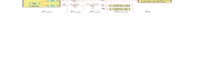
Figure 6: Modelling of the experiment.

The resulting Wigner function $W_{loss}$ is calculated by convolution of $W_{sqz}$ with the Wigner functions $W_{vac}$ of two vacuum modes, using $W_{vac}(x,p)=\exp(-x^{2}-p^{2})/\pi$. Then, the mode transmitted through the APD channel is mixed with another vacuum mode on a 50/50 beamsplitter, producing a density matrix $\rho_{mix}$ involving three modes $H$, $A$ and $B$, and associated with the Wigner function :

$W_{mix}$	=	$W_{loss}\left(x_{H},p_{H},\frac{x_{A}+x_{B}}{\sqrt{2}},\frac{p_{A}+p_{B}}{\sqrt{2}}\right)$
		$\times W_{vac}\left(\frac{x_{A}-x_{B}}{\sqrt{2}},\frac{p_{A}-p_{B}}{\sqrt{2}}\right)$

The modes $A$ and $B$ are detected by the APDs $A$ and $B$, which realize respectively the projective measurements $\Pi_{A,B}=Id-|0_{A,B}\rangle\langle 0_{A,B}|$ with a probability $\xi$ (“matched clicks”), and $\Pi_{0}=Id$ with a probability $1-\xi$ (“unmatched clicks”). The density matrix becomes

$$\rho_{cond} = N_{2}\xi^{2}\Pi_{A}\Pi_{B}\rho_{mix}\Pi_{A}\Pi_{B}+(1-\xi)^{2}\rho_{mix}$$

$$+N_{1}\xi(1-\xi)(\Pi_{A}\rho_{mix}\Pi_{A}+\Pi_{B}\rho_{mix}\Pi_{B})$$

where $N_{1}=1/Tr(\Pi_{A}\rho_{mix})=1/Tr(\Pi_{B}\rho_{mix})$ and $N_{2}=1/Tr(\Pi_{A}\Pi_{B}\rho_{mix})$. Finally, the density matrix of the measured two-photon state is obtained by tracing out the two APD modes $A$ and $B$ :

$$\rho_{2} = Tr_{A,B}\;\rho_{cond}$$ (11)

$$= \left[N_{2}\xi^{2}+2N_{1}\xi(1-\xi)+(1-\xi)^{2}\right]Tr_{A,B}\;\rho_{mix}$$

$$-\left[N_{2}\xi^{2}+N_{1}\xi(1-\xi)\right]Tr_{B}\langle 0_{A}|\rho_{mix}|0_{A}\rangle$$

$$-\left[N_{2}\xi^{2}+N_{1}\xi(1-\xi)\right]Tr_{A}\langle 0_{B}|\rho_{mix}|0_{B}\rangle$$

$$+N_{2}\xi^{2}\langle 0_{A}0_{B}|\rho_{mix}|0_{A}0_{B}\rangle$$

The associated Wigner function can be calculated using

$Tr_{K}W_{mix}$	=	$\int{W_{mix}}dx_{K}dp_{K}$
$\langle 0_{K}|W_{mix}|0_{K}\rangle$	=	$2\pi\int{W_{mix}W_{vac}}dx_{K}dp_{K}$

where $K=A,B$. As expected, it has no definite phase and depends only on $R^{2}=x_{H}^{2}+p_{H}^{2}$. It has the form

$$W_{2} = \frac{\alpha e^{-{\textstyle\frac{R^{2}}{\sigma_{2}^{2}}}}}{\pi\sigma_{2}^{2}}-\frac{\beta e^{-{\textstyle\frac{R^{2}}{\sigma_{1}^{2}}}}}{\pi\sigma_{1}^{2}}+\frac{(1-\alpha+\beta)e^{-{\textstyle\frac{R^{2}}{\sigma^{2}}}}}{\pi\sigma^{2}}$$ (12)

where $\alpha$, $\beta$ and $\sigma_{i}$ are functions of the parameters above. This linear combination of gaussian functions looks quite simple, but $\alpha$ and $\beta$ diverge when the OPA gain or the APD efficiency are small, which is our case. This leads to numerical instabilities when this expression is used for data analysis. To avoid this problem one can simply take the limit $\mu\rightarrow 0$ in eq. (12), obtaining eq. (1) quoted in the main text above. In our range of parameters, these two equations are numerically indistinguishable.