Generation of Entangled Two-Photons Binomial States
in Two Spatially Separate Cavities

Abstract

We propose a conditional scheme to generate entangled two-photons generalized binomial states inside two separate single-mode high-$Q$ cavities. This scheme requires that the two cavities are initially prepared in entangled one-photon generalized binomial states and exploits the passage of two appropriately prepared two-level atoms one in each cavity. The measurement of the ground state of both atoms is finally required when they exit the cavities. We also give a brief evaluation of the experimental feasibility of the scheme.

1. Introduction

Entanglement of separate systems certainly represents one of the most striking features of quantum physics, both for its fundamental nonlocal behavior [1, 2] and for its applications in quantum information processing [3, 4]. For these reasons, it is important to have implementable methods to generate entangled states between separate systems in various contexts.

In cavity quantum electrodynamics (CQED) several schemes, exploiting typical atom-cavity interactions, have been proposed to obtain, in two separate single-mode cavities, entangled one-photon number states [5, 6, 7, 8, 9]. In this context, it would be of interest to get entanglement between electromagnetic field states with mesoscopic characteristics and therefore having a maximum number of photons larger than one, so that the classical-quantum border may be investigated.

In this paper we propose a conditional scheme aimed at generating entangled two-photons generalized binomial states (2GBSs) inside two separate single-mode high-$Q$ cavities. Our scheme requires that the two cavities are initially prepared in entangled one-photon generalized binomial states [10]. In order to reach our goal, we exploit the passage of two appropriately prepared atoms one in each cavity and measure the atomic state of both atoms when they exit the cavities. We will show that the probability of success is larger than or equal to $1/2$, and depends on the degree of entanglement we wish establish between the two cavities. We also give a brief evaluation of the implementation of the scheme.

This paper is organized as follows: in Sec. 2. we recall the Jaynes-Cummings model that regulates the dynamics of the system and we illustrate the scheme to generate entangled 2GBSs in two separate cavities, briefly discussing its implementation; in Sec. 3. we summarize our conclusions.

2. Generation scheme

The generation scheme here proposed exploits the resonant interaction of a two-level atoms with a single-mode high-$Q$ cavity described by the usual Jaynes-Cummings Hamiltonian [11]

$$H_{JC}=\hbar\omega\sigma_{z}/2+\hbar\omega a^{{\dagger}}a+i\hbar g(\sigma_{+}a-\sigma_{-}a^{{\dagger}})$$ (1)

where $g$ is the atom-field coupling constant, $\omega$ is the resonant cavity field mode, $a$ and $a^{{\dagger}}$ are the field annihilation and creation operators and $\sigma_{z}=|\uparrow\rangle\langle\uparrow|-|\downarrow\rangle\langle\downarrow|$, $\sigma_{+}=|\uparrow\rangle\langle\downarrow|$, $\sigma_{-}=(\sigma_{+})^{{\dagger}}$ are the pseudo-spin operators, $|\uparrow\rangle$ and $|\downarrow\rangle$ being respectively the excited and ground state of the two-level atom. It is well known that the Hamiltonian $H_{JC}$ generates the evolutions [6, 12]

$$|\uparrow\rangle|n\rangle\equiv|\uparrow,n\rangle \rightarrow \cos(g\sqrt{n+1}t)|\uparrow,n\rangle-\sin(g\sqrt{n+1}t)|\downarrow,n+1\rangle$$

$$|\downarrow\rangle|n\rangle\equiv|\downarrow,n\rangle \rightarrow \cos(g\sqrt{n}t)|\downarrow,n\rangle+\sin(g\sqrt{n}t)|\uparrow,n-1\rangle,$$ (2)

where $a^{\dagger}a|n\rangle=n|n\rangle$.

The scheme we are going to discuss, illustrated for simplicity in Fig.1, follows standard procedures currently used for CQED experiments [13, 14].

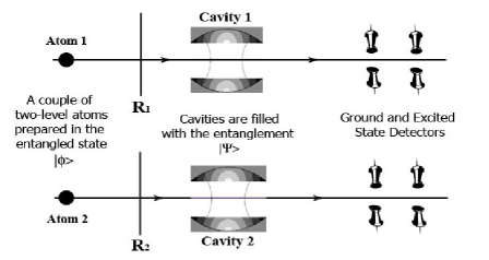
Fig. 1: Experimental scheme for the generation of entangled two-photons binomial states in two separate cavities.

We suppose that the two cavities are initially prepared in entangled orthogonal one-photon generalized binomial states given by [10]

$$|\Psi^{(1)}\rangle=\mathcal{N_{\eta}}\Big{[}|p_{1},\vartheta_{1}\rangle_{1}|1-p_{2},\pi+\vartheta_{2}\rangle_{2}+\eta|1-p_{1},\pi+\vartheta_{1}\rangle_{1}|p_{2},\vartheta_{2}\rangle_{2}\Big{]},$$ (3)

where $\eta\in\mathbb{R}$, ${\cal N}_{\eta}=1/\sqrt{1+|\eta|^{2}}$ is a normalization constant and the state

$$|p,\vartheta\rangle=\sqrt{1-p}|0\rangle+e^{i\vartheta}\sqrt{p}|1\rangle$$ (4)

represents the one-photon generalized binomial state with a probability of a single photon occurrence $p\in]0,1[$ and mean phase $\vartheta$ [15, 16]. In Eq. (3), $|p_{j},\vartheta_{j}\rangle_{j}$ denotes the single-mode state of the $j$-th cavity. The state $|\Psi^{(1)}\rangle$ can be deterministically obtained following, for example, the scheme reported in Ref. [10]. Consider now a couple of identical two-level Rydberg atoms in the entangled state

$$|\phi\rangle={\cal N}_{\eta}(|\uparrow_{1}\downarrow_{2}\rangle-\eta|\downarrow_{1}\uparrow_{2}\rangle).$$ (5)

This state can be prepared using, for example, the scheme suggested by Gerry [17]. Before entering the cavity $j$, the $j$-th atom crosses a Ramsey zone $R_{j}$ ($j=1,2$) where it resonantly interacts with a classical field undergoing the transformations

$$|\uparrow_{j}\rangle \rightarrow |\uparrow\rangle_{\mathbf{u}_{j}}\equiv\cos(\theta_{j}/2)|\uparrow_{j}\rangle-e^{i\varphi_{j}}\sin(\theta_{j}/2)|\downarrow_{j}\rangle$$

$$|\downarrow_{j}\rangle \rightarrow |\downarrow\rangle_{\mathbf{u}_{j}}\equiv e^{-i\varphi_{j}}\sin(\theta_{j}/2)|\uparrow_{j}\rangle+\cos(\theta_{j}/2)|\downarrow_{j}\rangle,$$ (6)

with the versor $\mathbf{u}\equiv(-\sin\theta\cos\varphi,-\sin\theta\sin\varphi,\cos\theta)$. As well known, by adjusting the amplitude of the classical Ramsey field as well as the interaction time between this field and the atom, we have the possibility to control both the two quantities $\theta$, the so-called “Ramsey pulse”, and $\varphi$. Stated another way, we can prepare an arbitrary superposition of the two atomic states $|\uparrow_{j}\rangle,|\downarrow_{j}\rangle$. Putting in particular

$$\cos(\theta_{j}/2)\equiv\sqrt{p_{j}},\ \sin(\theta_{j}/2)\equiv\sqrt{1-p_{j}};\ \varphi_{j}=-\vartheta_{j}$$ (7)

where $p_{1},p_{2},\vartheta_{1},\vartheta_{2}$ are the same parameters that appear in the entangled state $|\Psi^{(1)}\rangle$ of Eq. (3), the transformations of Eqs. (6) can be written as

$$|\uparrow_{j}\rangle \rightarrow |\uparrow\rangle_{\mathbf{u}_{j}}\equiv\sqrt{p_{j}}|\uparrow_{j}\rangle-e^{-i\vartheta_{j}}\sqrt{1-p_{j}}|\downarrow_{j}\rangle$$

$$|\downarrow_{j}\rangle \rightarrow |\downarrow\rangle_{\mathbf{u}_{j}}\equiv e^{i\vartheta_{j}}\sqrt{1-p_{j}}|\uparrow_{j}\rangle+\sqrt{p_{j}}|\downarrow_{j}\rangle.$$ (8)

Therefore, the total atom-cavity state after the Ramsey zones is

$$|\Phi(0)\rangle=\mathcal{N}_{\eta}\big{(}|\uparrow\rangle_{\mathbf{u}_{1}}|\downarrow\rangle_{\mathbf{u}_{2}}-\eta|\downarrow\rangle_{\mathbf{u}_{1}}|\uparrow\rangle_{\mathbf{u}_{2}}\big{)}|\Psi^{(1)}\rangle.$$ (9)

Successively each atom enters the respective cavity where it resonantly interacts with the single-mode electromagnetic field. The dynamics of the two subsystems “atom+cavity” 1 and 2 are independent. So, starting from the total atom-cavity state of Eq. (9) and using the explicit expressions of the cavity and atomic states given in Eqs. (3), (4), (8), we exploit the Jaynes-Cummings evolutions as given by Eq. (2) in correspondence to each subsystem $j=1,2$. Indicate by $T_{j}$ the interaction time between the atom $j$ and the $j$-th cavity, and suppose that the conditions

$$\sin gT_{j}+\cos gT_{j}=\sqrt{2},\quad\sin(g\sqrt{2}T_{j})=1$$ (10)

are satisfied. Under these hypothesis we obtain

$$|\uparrow\rangle_{\mathbf{u}_{j}}|p_{j},\vartheta_{j}\rangle_{j} \stackrel{{\scriptstyle T_{j}}}{{\rightarrow}} -e^{-i\vartheta_{j}}|2,p_{j},\vartheta_{j}\rangle_{j}|\downarrow_{j}\rangle,$$

$$|\downarrow\rangle_{\mathbf{u}_{j}}|p_{j},\vartheta_{j}\rangle_{j} \stackrel{{\scriptstyle T_{j}}}{{\rightarrow}} \frac{1}{\sqrt{2}}\big{[}e^{i\vartheta_{j}}|0_{j}\uparrow_{j}\rangle+|\Gamma_{j}(p_{j},\vartheta_{j})\rangle\big{]},$$

$$|\uparrow\rangle_{\mathbf{u}_{j}}|1-p_{j},\pi+\vartheta_{j}\rangle_{j} \stackrel{{\scriptstyle T_{j}}}{{\rightarrow}} \frac{1}{\sqrt{2}}\big{[}|0_{j}\uparrow_{j}\rangle-e^{-i\vartheta_{j}}|\Gamma_{j}(p_{j},\vartheta_{j})\rangle\big{]},$$

$$|\downarrow\rangle_{\mathbf{u}_{j}}|1-p_{j},\pi+\vartheta_{j}\rangle_{j} \stackrel{{\scriptstyle T_{j}}}{{\rightarrow}} |2,1-p_{j},\pi+\vartheta_{j}\rangle_{j}|\downarrow_{j}\rangle,$$ (11)

where we have indicated with $|2,p,\vartheta\rangle$ the generalized binomial state with a maximum number of photons $N=2$, probability of a single photon occurrence $p$ and mean phase $\vartheta$, defined as [15, 16]

$$|2,p,\vartheta\rangle\equiv\sum_{n=0}^{2}\left[{2\choose n}p^{n}(1-p)^{2-n}\right]^{1/2}e^{in\vartheta}|n\rangle,$$ (12)

and where we have set

$$|\Gamma_{j}(p_{j},\vartheta_{j})\rangle\equiv\sqrt{2p_{j}(1-p_{j})}|0_{j}\rangle-(1-2p_{j})e^{i\vartheta_{j}}|1_{j}\rangle-\sqrt{2p_{j}(1-p_{j})}e^{2i\vartheta_{j}}|2_{j}\rangle.$$ (13)

Unfortunately the conditions of Eq. (10) cannot be simultaneously satisfied. Let us however observe that, solving the first condition of Eq. (10), we get $gT_{j}=\pi/4+2m_{j}\pi$, where $m_{j}$ is a non-negative integer. Thus we can look for suitable values of $m_{j}$ in correspondence of which the second condition of Eq. (10) is approximatively satisfied. The choice of $m_{j}$ however must be done coherently with the typical experimental values of the interaction times in CQED systems ($gT_{j}\sim 10^{-1}\div 10^{2}$ [13]), thus confining the values of $m_{j}$ inside the range $0\leq m_{j}\leq 16$. Fixing, in particular, $m_{j}=5$ and therefore the same interaction time in the two cavities given by

$$T_{1}=T_{2}=T=41\pi/4g,$$ (14)

we find that

$$\sin(g\sqrt{2}T)=1-\delta,\ \textrm{where $\delta\sim 10^{-4}$}.$$ (15)

Within this approximation we can consider the second condition of Eq. (10) as satisfied, too. So, utilizing Eq. (11) with $T_{j}=T$, we find that, if the condition $\vartheta_{1}=\vartheta_{2}\equiv\vartheta$ is verified, the total atom-cavity state $|\Phi(0)\rangle$ of Eq. (9) evolves, apart from a global phase factor, into

$$|\Phi(T)\rangle = \mathcal{N}_{\eta}^{2}\big{\{}\big{[}|2,p_{1},\vartheta\rangle_{1}|2,1-p_{2},\pi+\vartheta\rangle_{2}-\eta^{2}|2,1-p_{1},\pi+\vartheta\rangle_{1}|2,p_{2},\vartheta\rangle_{2}\big{]}|\downarrow_{1}\downarrow_{2}\rangle$$ (16)

$$- \eta e^{i\vartheta}|0_{1}\rangle|\Gamma_{2}(p_{2},\vartheta)\rangle|\uparrow_{1}\downarrow_{2}\rangle+\eta e^{i\vartheta}|\Gamma_{1}(p_{1},\vartheta)\rangle|0_{2}\rangle|\downarrow_{1}\uparrow_{2}\rangle\big{\}}.$$

From Eq. (16), it is readily noticed that, if both atoms are measured in the ground state $|\downarrow\rangle$ after exiting the cavities, the resulting two-cavities field state is

$$|\Psi^{(2)}\rangle=\mathcal{N}_{2}\big{[}|2,p_{1},\vartheta\rangle_{1}|2,1-p_{2},\pi+\vartheta\rangle_{2}-\eta^{2}|2,1-p_{1},\pi+\vartheta\rangle_{1}|2,p_{2},\vartheta\rangle_{2}\big{]}.$$ (17)

Since it is satisfied the orthogonality condition $\langle 2,p,\vartheta|2,1-p,\pi+\vartheta\rangle=0$ [10], the normalization constant has the value $\mathcal{N}_{2}=1/\sqrt{1+|\eta|^{4}}$, and the state $|\Psi^{(2)}\rangle$ of Eq. (17) represents entangled orthogonal 2GBSs in two separate single-mode high-$Q$ cavities. From Eq. (16), the probability of finding both atoms in the ground state after exiting the cavities, i.e. the probability of success to obtain our target state $|\Psi^{(2)}\rangle$, is given by

$$\mathcal{P}_{succ}=|\langle\Psi^{(2)}|\langle\downarrow_{1}\downarrow_{2}|\Phi(T)\rangle|^{2}=\mathcal{N}_{\eta}^{4}/\mathcal{N}_{2}^{2}\Rightarrow\mathcal{P}_{succ}=(1+|\eta|^{4})/(1+|\eta|^{2})^{2}.$$ (18)

Following Ref. [18], the degree of entanglement of the state $|\Psi^{(2)}\rangle$ is given by $G^{(E)}=2|\eta|^{2}/(1+|\eta|^{4})$ and it is invariant with respect to the substitution $|\eta|\rightarrow 1/|\eta|$, equal to zero for $|\eta|=0,+\infty$ (uncorrelated states) and equal to one for $|\eta|=1$ (maximally entangled states). In terms of $G^{(E)}$, the probability of success $\mathcal{P}_{succ}$ given in Eq. (18) becomes $\mathcal{P}_{succ}=1/\big{(}1+G^{(E)}\big{)}$. In Fig.2 we plot the graph of $\mathcal{P}_{succ}$ versus the parameter of entanglement $|\eta|$.

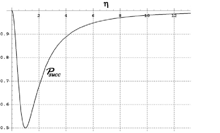
Fig. 2: Plot of the probability $\mathcal{P}_{succ}$ to obtain entangled two-photons binomial states in function of the parameter of entanglement $|\eta|\in[0,+\infty[$.

The probability of success to obtain maximally entangled 2GBSs, when $|\eta|=G^{(E)}=1$, has its minimum value $\mathcal{P}_{succ}^{(min)}=1/2$ and it tends to one when $|\eta|\rightarrow 0,+\infty$, i.e. when the degree of entanglement $G^{(E)}$ tends to zero. The probability of success is equal to one for $|\eta|=0,+\infty$, but in this case, with $G^{(E)}=0$, there is no entanglement at all.

As remarked, the state $|\Psi^{(2)}\rangle$ of Eq. (17) represents entangled two-photons generalized binomial states. However, when the probabilities of a single photon occurrence $p_{j}$ ($j=1,2$) take their limit values $p_{j}=0,1$, the state $|\Psi^{(2)}\rangle$ reduces to entangled number states with zero or two photons inside the cavities. In fact, using the property that a binomial state with a maximum number of photons $N$ is equal to $|0\rangle$ for $p=0$ and to $|N\rangle$ for $p=1$ [15], from Eq. (17) we obtain

$$|\Psi^{(2)}\rangle_{p_{1}=p_{2}=1} = \mathcal{N}_{2}\big{[}|2_{1}0_{2}\rangle-\eta^{2}|0_{1}2_{2}\rangle\big{]},$$

$$|\Psi^{(2)}\rangle_{p_{1}=1,p_{2}=0} = \mathcal{N}_{2}\big{[}|2_{1}2_{2}\rangle-\eta^{2}e^{-4i\vartheta}|0_{1}0_{2}\rangle\big{]}.$$ (19)

We shall give here a brief evaluation of some experimental errors involved in the implementation of our generation scheme. A necessary condition required by this scheme is that the atoms cross the cavities for a predeterminate time $T$. The experimental uncertainties on selected velocity and interaction time, $\Delta v$ and $\Delta T$, are such that $\Delta T/T\approx\Delta v/v$. In current laboratory experiments we have $\Delta v/v\sim 10^{-2}$ or less [14, 19]. It is also possible to see that the error $\delta$ of Eq. (15) is much smaller than the error induced by these experimental values of $\Delta T/T$ on the condition $\sin(g\sqrt{2}T)=1$. Another aspect we have ignored is the atomic or photon decay during the atom-cavity interactions. This assumption is valid if $\tau_{at},\tau_{cav}>T$, where $\tau_{at},\tau_{cav}$ are the atomic and photon mean lifetimes respectively and $T$ is the interaction time. For Rydberg atomic levels and microwave superconducting cavities with quality factor $Q\sim 10^{8}\div 10^{10}$, we have $\tau_{at}\sim 10^{-5}\div 10^{-2}\textrm{s}$ and $\tau_{cav}\sim 10^{-4}\div 10^{-1}\textrm{s}$. Since typical atom-cavity field interaction times are $T\sim 10^{-5}\div 10^{-4}\textrm{s}$, the required condition on the mean lifetimes can be satisfied [13]. Moreover, the typical mean lifetimes of the Rydberg atomic levels $\tau_{at}$ must be such that the atoms do not decay during the entire sequence of the scheme and, since the proposed scheme requires that the cavities are initially prepared in entangled one-photon generalized binomial states [10], the photon mean lifetimes $\tau_{cav}$ must be long enough to permit cavity fields not to decay before they interact with the successive atoms [13, 14]. Finally, we should consider the fact that experimental detectors efficiencies are smaller than one, so we could have no “click” when an atom crosses the field ionization detector: in this case the generation scheme should be repeated from the beginning.

3. Conclusion

In this paper we have proposed a conditional scheme for the generation of entangled two-photons generalized binomial states in two spatially separate single-mode high-$Q$ cavities. This scheme exploits standard atom-cavity interactions and requires the final measurement of the atomic states. The probability of success to generate our target state is always larger than or equal to $1/2$, depending on the value of the parameter of entanglement $|\eta|$ and therefore on the degree of entanglement $G^{(E)}$. In particular, we have seen that the probability of success to obtain maximally entangled two-photons binomial states, i.e. when $|\eta|=G^{(E)}=1$, takes its minimum value $\mathcal{P}_{succ}^{(min)}=1/2$ and it tends to one when $G^{(E)}$ tends to zero.

Finally, we have briefly estimated the typical experimental errors involved in such CQED systems, and we have seen that our generation scheme is not sensibly affected by these errors. This shows that the implementation of our generation scheme is within the current experimental technics [14].

As far as we know, the scheme proposed here for the generation of entangled two-photons generalized binomial states in two separate cavities represents the first example, in the context of the CQED, of a scheme that permits to produce entanglement between non-classical states of the electromagnetic field having non zero mean fields and a number of photons greater than one. In conclusion, this kind of entangled state could be useful for fundamental investigations on nonlocal properties, for studying field correlations between the cavities or Bell’s inequality violations, and for applications in quantum computation and information processing.

References

• [1] A. Einstein, B. Podolsky, N. Rosen, Phys. Rev. 47, 777 (1935).
• [2] J.S. Bell, Physics 1, 195 (1964).
• [3] C. H. Bennett, G. Brassard, C. Crepeau, R. Jozsa, A. Peres, and W. K. Wootters, Phys. Rev. Lett. 70, 1895 (1993).
• [4] J. Preskill, Lecture Notes for Physics 229: Quantum Information and Computation, http://theory.caltech.edu/~preskill/ph229 (1998).
• [5] J. A. Bergou, M. Hillery, Phys. Rev. A 55, 4585 (1997).
• [6] P. Meystre, in Progress in Optics XXX: Cavity Quantum Optics and the Quantum Measurement process, edited by E. Wolf (Elsevier Science Publishers B.V., New York, 1992).
• [7] A. Messina, Eur. Phys. J. D 18, 379 (2002).
• [8] A. Napoli, A. Messina, G. Compagno, Fortschr. Phys. 51, 81 (2003).
• [9] D.E. Browne, M.B. Plenio, Phys. Rev. A 67, 012325 (2003).
• [10] R. Lo Franco, G. Compagno, A. Messina and A. Napoli, Phys. Rev. A 72, 053806 (2005).
• [11] E. T. Jaynes and F. W. Cummings, P.I.E.E.E. 51, 89 (1963).
• [12] P. Carbonaro, G. Compagno and F. Persico, Phys. Lett. A 73, 97 (1979).
• [13] S. Haroche, in Les Houches Session LIII 1990, Systémes Fondamentaux en Optique Quantique: Course 13, Cavity Quantum Electrodynamics (Elsevier Science Publishers B.V., New York, 1992).
• [14] S. Haroche, Phys. Scripta 102, 128-132 (2002).
• [15] D. Stoler, B. E. A. Saleh and M. C. Teich, Opt. Acta 32, 345 (1985).
• [16] A. Vidiella-Barranco, J.A. Roversi, Phys. Rev. A 67, 5233 (1994).
• [17] C. C. Gerry, Phys. Rev. A 53, 4583 (1996).
• [18] A. F. Abouraddy, B. E. A. Saleh, A. V. Sergienko, and M. C. Teich, Phys. Rev. A 64, 050101 (2001).
• [19] E. Hagley, et al., Phys. Rev. Lett. 79, 1 (1997).