Relations among Quantum Processes: Bisimilarity and Congruence

Abstract

Full formal descriptions of algorithms making use of quantum principles must take into account both quantum and classical computing components, as well as communications between these components. Moreover, to model concurrent and distributed quantum computations and quantum communication protocols, communications over quantum channels which move qubits physically from one place to another must also be taken into account.

Inspired by classical process algebras, which provide a framework for modeling cooperating computations, a process algebraic notation is defined. This notation provides a homogeneous style to formal descriptions of concurrent and distributed computations comprising both quantum and classical parts. Based upon an operational semantics which makes sure that quantum objects, operations and communications operate according to the postulates of quantum mechanics, an equivalence is defined among process states considered as having the same behavior. This equivalence is a probabilistic branching bisimulation. From this relation, an equivalence on processes is defined. However, it is not a congruence because it is not preserved by parallel composition.

1 Introduction

The number of quantum programming languages is growing rapidly. These languages can be classified in three families: imperative, functional, and parallel and distributed. Among imperative programming languages, there are QCL [Ömer 2000], designed by Ömer, which aims at simulating quantum programs, and qGCL [Zuliani 2001] by Zuliani which allows the construction by refinement of proved correct quantum programs. QPL [Selinger 2004] is a functional language designed by Selinger with a denotational semantics. Several quantum $\lambda$-calculi have also been developed: for example [van Tonder 2003] by Van Tonder, based on a simplified linear $\lambda$-calculus and [Arrighi and Dowek 2004] by Arrighi and Dowek, which is a ”linear-algebraic $\lambda$-calculus”. Gay and Nagarajan have developed CQP, a language to describe communicating quantum processes [Nagarajan and Gay 2004]. This language is based on $\pi$-calculus. An important point in their work is the definition of a type system, and the proof that the operational semantics preserves typing.

Cooperation between quantum and classical computations is inherent in quantum algorithmics. Teleportation of a qubit state from Alice to Bob [Bennett et al. 1993] is a good example of this cooperation. Indeed, Alice carries out a measurement, the result of which (two bits) is sent to Bob, and Bob uses this classical result to determine which quantum transformation he must apply. Moreover, initial preparation of quantum states and measurement of quantum results are two essential forms of interactions between the classical and quantum parts of computations which a language must be able to express. Process algebras are a good candidate for such a language since they provide a framework for modeling cooperating computations. In addition, they have well defined semantics and permit the transformation of programs as well as the formal study and analysis of their properties. Their semantics give rise to an equivalence relation on processes. Bisimilarity is an adequate equivalence relation to deal with communicating processes since it relates processes that can execute the same flows of actions while having the same branching structure.

This paper presents first the main points of the definition and semantics of a Quantum Process Algebra (QPAlg). Then, a probabilistic branching bisimilarity is defined among process states (section 3), this relation is proved to be an equivalence. As an example, in section 4, the application of the Hadamard unitary transformation is proved bisimilar with its simulation with measurement only, based on state transfer. Finally, in section 5, an equivalence relation among processes is defined. This relation is preserved by all the operators of QPAlg except parallel composition.

2 Definition of QPAlg

The process algebra QPAlg is based upon process algebras such as CCS [Milner 1989] and Lotos [Bolognesi and Brinksma 1987]. The key aspects of QPAlg are developed in this section. The precise syntax and the main inference rules of the semantics are given in appendix A. For more details and more examples, see [Lalire and Jorrand 2004].

2.1 Variables

For the purpose of this paper, we consider two types of variables, one classical: $\mathtt{Nat}$, for variables taking natural values, and one quantum: $\mathtt{Qubit}$ for variables standing for qubits. An extended version of the process algebra would of course also include quantum registers and other types of variables.

In classical process algebras with value passing [Milner 1989, Bolognesi and Brinksma 1987, Roscoe 1998], variables are instantiated when communications between processes occur and cannot be modified after their instantiation. As a consequence, it is not necessary to store their values. In fact, when a variable is instantiated, all its occurrences are replaced by the value received.

Here, quantum variables represent physical qubits. Applying a transformation to a variable which represents a qubit modifies the state of that qubit. This means that values of variables are modified. For that reason, a process state must keep track of both variable names and variable states, this is achieved thanks to the context (cf. section 2.5).

Variables are declared using the following syntax: $\boldsymbol{[}\ x_{1}:t_{1},\ldots,x_{n}:t_{n}\boldsymbol{\ }.\ P\ \boldsymbol{]}$ where $x_{1},\ldots,x_{n}$ is a list of variables, $t_{1},\ldots,t_{n}$ are their types, and $P$ is a process which can make use of these classical and quantum variables.

2.2 Expressions

The quantum expressions are quantum variables or tensor product of quantum variables, denoted $x_{1}\otimes\cdots\otimes x_{n}$.

The classical expressions are usual classical expressions, and application of an admissible transformation to a quantum expression. Admissible transformations are also called general quantum measurements, it includes unitary transformations. For more details, see [Nielsen and Chuang 2000].

Let $\mathcal{A}$ be a set of predefined admissible transformations. The application of the admissible transformation $A=\{A_{\tau_{1}},\ldots,A_{\tau_{m}}\}\in\mathcal{A}$, of dimension $n$, to the register of qubits $x_{1}\otimes\cdots\otimes x_{n}$ is denoted $A[x_{1}\otimes\cdots\otimes x_{n}]$.

The quantum memory is stored in the context in the form $q=\rho$ where $q$ is the list of quantum variable names and $\rho$, a density matrix representing their quantum state (cf. section 2.5). If the classical result of $A[x_{1}\otimes\cdots\otimes x_{n}]$ is $\tau_{i}$, then $\mathcal{T}_{A_{\tau_{i}}}$ is the super-operator which must be applied to the density matrix $\rho$, to describe the evolution of the quantum memory $q=\rho$.

$$\mathcal{T}_{A_{\tau_{i}}}:\rho\mapsto\Pi^{\dagger}.(A_{\tau_{i}}\otimes I^{\otimes k}).\Pi.\rho.\Pi^{\dagger}.(A_{\tau_{i}}^{\dagger}\otimes I^{\otimes k}).\Pi$$

where

• $\Pi$ is the permutation matrix which places the $x_{i}$’s at the head of $q$

• $k=\mathtt{size}(q)-n\$

• $I^{\otimes k}\!=\underbrace{I\otimes\cdots\otimes I}_{k}$, where $I$ is the identity matrix on $\mathbb{C}^{2}$

Since the admissible transformation $A_{\tau_{i}}$ may be applied to qubits which are anywhere within the list $q$, a permutation $\Pi$ must be applied first. This permutation moves the $x_{i}$’s so that they are placed at the head of $q$ in the order specified by $x_{1},\ldots,x_{n}$. Then $A_{\tau_{i}}$ can be applied to the first $n$ elements and $I$ to the remainder. Finally, the last operation is the inverse of the permutation $\Pi$ so that at the end, the arrangement of the elements in $\rho$ is consistent with the order of the elements in $q$.

$A[x_{1}\otimes\cdots\otimes x_{n}]$ is not probabilistic but its evaluation produces a result with a probabilistic value. This value is stored in the context which becomes probabilistic (cf. section 2.5).

In the examples of this paper, the set $\mathcal{A}$ of admissible transformations is:

$$\mathcal{A}=\{H,CNot,I,\sigma_{X},\sigma_{Y},\sigma_{Z},M_{std,1},M_{std,2},X,Z\otimes X\}$$

$H$ is Hadamard transformation, $CNot$ is ”controlled not”, $I$ is the identity, and $\sigma_{X}$, $\sigma_{Y}$, $\sigma_{Z}$ are Pauli operators. $M_{std,1}$ and $M_{std,2}$ correspond to measurement in the standard basis of respectively one and two qubits. $X$ and $Z\otimes X$ are the admissible transformations corresponding to the measurements with the Pauli observables $X$ and $Z\otimes X$.

2.3 Basic actions

The basic actions of QPAlg are classical expressions and communications. A classical expression is interesting as a basic action if it has side effects, as it is the case of the application of an admissible transformation.

There are several kinds of communications, depending on the type of the expression sent and the type of the receiving variable. The different kinds of communications are: classical to classical communications, classical to quantum communications for initializing qubits, and quantum to quantum communications for allowing the description of quantum communication protocols. Communication gates are not typed but we can imagine a subsequent version of QPAlg where communication gates would be declared with a fixed type like the other variables.

Emission of an expression $e$ from a gate $g$ is denoted $g\ !e\$, reception in a variable $x$ is denoted $g\ ?x\$. In the operational semantics of parallel composition (rules 15 to 20 of the semantics given in appendix A.2), the combination of the rules for emission and reception defines communication. In a classical to quantum communication (rule 17), the qubit is initialized in the basis state $|v\rangle\langle v|$, where $v$ is the classical value sent (in this case, $v$ must be $0$ or $1$). In a quantum to quantum communication (rule 18), the name of the sent qubit is replaced in the context by the name of the receiving qubit.

2.4 Composition operators

To create a process from basic actions, the prefix operator ”” is used: if $\alpha$ is an action and $P$, a process, $\alpha P$ is a new process which performs $\alpha$ first, then behaves as $P$.

The predefined process nil cannot perform any transition.

The operators of the process algebra are: parallel composition ($P\parallel Q$), nondeterministic choice ($P+Q$), probabilistic choice ($P\oplus_{p}Q$), conditional choice ($\boldsymbol{[}\ c_{1}\rightarrow P_{1},\ldots,c_{n}\rightarrow P_{n}\ \boldsymbol{]}$) and restriction ($P\backslash L\$). The process $\boldsymbol{[}\ c_{1}\rightarrow P_{1},\ldots,c_{n}\rightarrow P_{n}\ \boldsymbol{]}$, where $c_{i}$ is a condition and $P_{i}$ a process, evolves as a process chosen nondeterministically among the processes $P_{j}$ such that $c_{j}$ is true. Restriction is useful for disallowing the use of some gates (the gates listed in $L$), thus forcing internal communication within process $P$. Communication can occur between two parallel processes whenever a value emission in one of them and a value reception in the other one use the same gate name.

The process $P\oplus_{p}Q$ behaves like $P$ with probability $p$ and like $Q$ with probability $1-p$. As explained in [Cazorla et al. 2001] and [Cazorla et al. 2003] and shown in the example of figure 1, if a process contains both a probabilistic and a nondeterministic choice, then the probabilistic choice must always be solved first. Otherwise, a probabilistic transition labeled with a probability $p$ does not mean that this transition will be executed with probability $p$.

Figure 1: Nondeterminism solved before probabilistic choice

To solve probabilistic choices before nondeterministic ones, the notion of stability for processes is defined.

Definition 1

Probabilistic stability is defined by induction:

1. nil, $aP$, $\boldsymbol{[}\ x_{1}:t_{1},\ldots x_{n}:t_{n}\boldsymbol{\ }.\ P\ \boldsymbol{]}$ are stable.

2. $P\backslash L\$, $\boldsymbol{[}\ x_{1}:t_{1},\ldots,x_{n}:t_{n}\ \boldsymbol{]}\bullet P[a_{1},\ldots,a_{n}]$ are stable if and only if $P$ is stable.

3. $P+Q$, $P\parallel Q$ are stable if and only if $P$ and $Q$ are stable.

4. $\boldsymbol{[}\ c_{1}\rightarrow P_{1}\ldots c_{n}\rightarrow P_{n}\ \boldsymbol{]}$ is stable if and only if for all $i$, $P_{i}$ is stable.

$P$ stable is denoted $P\downarrow$.

In the examples, another operator on processes is used: ”$\ ;$”, for sequential composition. $P\ ;Q$ behaves like $Q$ once $P$ has terminated. This require the introduction of a predefined process end, for signaling successful termination. The operator ”;” can be simulated with ”$\parallel$”: $P\ ;Q$ behaves as $(P\parallel\delta?Q)\backslash\{\delta\}\$ where $\delta$ is a fresh gate name and with $\mbox{\it end}\displaystyle\mathop{=}^{\mathtt{def}}\delta!\mbox{\it nil}$.

2.5 Contexts and process states

In the inference rules which describe the semantics of processes, the states of processes are process terms $P$ together with contexts $C$, of the form $P/C$. The main purpose of a context is to maintain the quantum state, stored as $q=\rho$ where $q$ is a sequence of quantum variable names and $\rho$ a density matrix representing their current quantum state. In order to treat classical variables in a similar way, modifications of classical variables are allowed. So, for the same reason as in the case of quantum variables, classical values are stored in the context. Storing and retrieving classical values is represented by functions $f:\mbox{\it names}\rightarrow\mbox{\it values}$. The context keeps track of the embedding of variable scopes. To keep track of parallel composition, this is done via a ”cactus stack” structure of sets of variables, called the environment stack ($s$), which stores variable scopes and types. The set of all the variables in $s$ is denoted $\mathtt{Var}(s)$, ”.” adds an element on top of a stack, and ”$|$” concatenates two stacks.

Definition 2

A context is a tuple $<s,q=\rho,f>$, where:

• $s$ is the environment stack;

• $q$ is a sequence of quantum variable names;

• $\rho$ is a density matrix representing the quantum state of the variables in $q$;

• $f$ is the function which associates values with classical variables.

The evaluation of an admissible transformation (rule 2 of the semantics) produce a probabilistic result. This requires the introduction of a probabilistic composition operator for contexts. This operator is denoted $\boxplus_{p}$: the state $P/C_{1}\boxplus_{p}C_{2}$ is $P/C_{1}$ with probability $p$ and $P/C_{2}$ with probability $1-p$. In general, a context is either of the form $<s,q=\rho,f>$, or of the form $\mathop{\boxplus}_{p_{i}}\!\!<s_{i},q_{i}=\rho_{i},f_{i}>$ where the $p_{i}$’s are probabilities adding to $1$.

As in the case of probabilities introduced by the operator $\oplus_{p}$, so as to guarantee that probabilistic choice is always solved first, the notion of probabilistic stability for contexts is introduced: a context $C$ is probabilistically stable, which is denoted $C\downarrow$, if it is of the form $<s,q=\rho,f>$. If the context of a process state is not stable, a probabilistic transition must be performed first (rule 10 of the semantics).

2.6 Example: teleportation

The teleportation protocol [Bennett et al. 1993] transfers the state of a qubit in a place $A$ into a qubit in a place $B$ with only two classical bits sent from place $A$ to place $B$:

Once upon a time, there were two friends, Alice and Bob who had to separate and live away from each other. Before leaving, each one took a qubit of the same EPR pair. Then Bob went very far away, to a place that Alice did not know. Later on, someone gave Alice a mysterious qubit in a state $|\psi\rangle=\alpha|0\rangle+\beta|1\rangle$, with a mission to forward this state to Bob. Alice could neither meet Bob and give him the qubit, nor clone it and broadcast copies everywhere, nor obtain information about $\alpha$ and $\beta$. Nevertheless, Alice succeeded thanks to the EPR pair and the teleportation protocol.

This protocol is described with QPAlg in program 1.

$\begin{array}[]{rcl}\mbox{\bf BuildEPR}&\displaystyle\mathop{=}^{\mathtt{def}}&\boldsymbol{[}\ x:\mathtt{Qubit},y:\mathtt{Qubit}\ \boldsymbol{]}\bullet\\ &&\hskip 20.0pt((g_{1}\ ?x\ g_{2}\ ?y\ H[x]CNot[x,y]\mbox{\it end})\\ &&\hskip 20.0pt\parallel(g_{1}\ !0\ g_{2}\ !0\ \mbox{\it end}))\backslash\{g_{1},g_{2}\}\\ &&\\ \mbox{\bf Alice}&\displaystyle\mathop{=}^{\mathtt{def}}&\boldsymbol{[}\ x:\mathtt{Qubit},y:\mathtt{Qubit}\ \boldsymbol{]}\bullet\\ &&\hskip 20.0ptCNot[x,y]H[x]g\ !M_{std,2}[x,y]\ \mbox{\it end}\\ &&\\ \mbox{\bf Bob}&\displaystyle\mathop{=}^{\mathtt{def}}&\boldsymbol{[}\ z:\mathtt{Qubit}\ \boldsymbol{]}\bullet\\ &&\hskip 20.0pt\boldsymbol{[}\ k:\mathtt{Nat}\boldsymbol{\ }.\\ &&\hskip 20.0pt\hskip 20.0ptg\ ?k\\ &&\hskip 20.0pt\hskip 20.0pt\boldsymbol{[}\ k=0\rightarrow I[z]\mbox{\it end},\\ &&\hskip 20.0pt\hskip 20.0ptk=1\rightarrow\sigma_{X}[z]\mbox{\it end},\\ &&\hskip 20.0pt\hskip 20.0ptk=2\rightarrow\sigma_{Z}[z]\mbox{\it end},\\ &&\hskip 20.0pt\hskip 20.0ptk=3\rightarrow\sigma_{Y}[z]\mbox{\it end}\ \boldsymbol{]}\\ &&\hskip 20.0pt\boldsymbol{]}\\ &&\\ \mbox{\bf Teleport}&\displaystyle\mathop{=}^{\mathtt{def}}&\boldsymbol{[}\ \psi:\mathtt{Qubit}\ \boldsymbol{]}\bullet\\ &&\hskip 20.0pt\boldsymbol{[}\ a:\mathtt{Qubit},b:\mathtt{Qubit}\boldsymbol{\ }.\\ &&\hskip 20.0pt\hskip 20.0pt\mbox{\bf BuildEPR}[a,b]\ ;\\ &&\hskip 20.0pt\hskip 20.0pt(\mbox{\bf Alice}[\psi,a]\parallel\mbox{\bf Bob}[b])\backslash\{g\}\\ &&\hskip 20.0pt\boldsymbol{]}\\ \end{array}$

Program 1 Implementation of the teleportation protocol

The inference rules can be used to show that this protocol results in Bob’s $z$ qubit having the state initially possessed by the $x$ qubit of Alice, with only two classical bits sent from Alice to Bob.

3 Probabilistic branching bisimilarity

The operational semantics associates a process graph with a process state. A process graph is a set of transitions between process states, and an initial state [Fokkink 2000]. The transitions are action transitions: $S\xrightarrow{\ a\ }T$ where $S$, $T$ are states, and $a$ is an action (possibly the internal action $\tau$), or probabilistic transitions: $S\longrightarrow_{p}T$, where $p$ is a probability.

In this section, an equivalence relation on process states is defined: probabilistic branching bisimilarity, which identifies states when they are associated with process graphs having the same branching structure. The bisimilarity defined here is probabilistic because of the probabilistic transitions introduced by quantum measurement and by the operator of probabilistic choice. The choice of a branching bisimilarity comes from the fact that it abstracts from silent transitions (contrary to strong bisimilarity), but is finer than any other equivalence taking into account silent steps [van Glabbeek 1993].

This definition is inspired from the definitions in [Fokkink 2000] and [Andova 1999].

3.1 Preliminary definitions and notations

Process states

The set of all possible process states is denoted $\mathcal{S}$. Let $S,T\in\mathcal{S}$, then $S$ can be written $P/C_{P}$ and $T$, $Q/C_{Q}$ where $P$, $Q$ are process terms and $C_{P}$, $C_{Q}$ contexts (possibly probabilistic).

Assuming that $S=P/C_{P}$ and $C_{P}=<s,q=\rho,f>$, if $x$ is an initialized qubit in $S$, i.e. $(x,\mathtt{Qubit})\in s$ and $x\in q$, then $\rho_{x}^{S}$ is the state of $x$ and this state can be obtained with a trace out operation on $\rho$:

$$\rho_{x}^{S}=Tr_{\{x\}/q}(\rho)$$

Silent transitions

The transitions considered as silent are of course internal transitions ($\displaystyle\ \mathop{\longrightarrow}^{\tau}\$) but also probabilistic transitions. The reason is that we want, for example, the states $S_{1}$ and $S_{2}$ described in figure 2 to be equivalent.

Figure 2: Equivalent states

Silent transitions will be denoted $\leadsto$. $\leadsto^{*}$ stands for a sequence (possibly empty) of silent transitions, and $\leadsto^{0..1}$ stands for zero or one silent transition.

Function $\mu$

Let $\mathcal{R}$ be an equivalence on process states, $S$ be a process state and $\bar{S}$, its equivalence class with respect to $\mathcal{R}$. If $M$ is a set of process states, then $S\triangleright M$ means that there exists a sequence of transitions remaining in $M\cup\bar{S}$, from $S$ to a state in $M$.

A function $\mu_{\mathcal{R}}:\mathcal{S}\times\mathcal{P}(\mathcal{S})\rightarrow[0,1]$ is defined: $\mu_{\mathcal{R}}:(S,M)\mapsto p$, where $p$ is the probability to reach a state in the set $M$ from a state $S$ without leaving $\bar{S}\cup M$.

It should be noted that, for this function to yield a probability, nondeterminism must be eliminated in a way which allows the computation of $\mu$. Here, nondeterminism is treated as equiprobability, but this is just a convention for the definition of $\mu_{\mathcal{R}}$. For example, this does not imply the equivalence of the two process states $S_{1}$ and $S_{2}$ described in figure 3.

Figure 3: Non equivalent states

The function $\mu_{\mathcal{R}}$ is defined as follows:

• if $S\in M$ then $\mu_{\mathcal{R}}(S,M)=1$

• (3cm,6cm)(0cm,2cm)[r][r] else if $\exists\ T\in M\cup\bar{S}$ such that $S\longrightarrow_{p}T\triangleright M$ then let $E_{S}=\{R\in M\cup\bar{S}\ |\ S\longrightarrow_{p_{{}_{R}}}R\triangleright M\}$ in

  $$\mu_{\mathcal{R}}(S,M)=\sum_{R\in E_{S}}p_{{}_{R}}\ \mu_{\mathcal{R}}(R,M)$$

• (3cm,6cm)(0cm,2.5cm)[r][r] else if $\exists\ T\in M\cup\bar{S}$ such that $S\mbox{$\displaystyle\ \mathop{-\!-\longrightarrow}^{a}\ $}T\triangleright M$ then let $E_{S}=\{R\in M\cup\bar{S}\ |\ S\mbox{$\displaystyle\ \mathop{-\!-\longrightarrow}^{a_{{}_{R}}}\ $}R\triangleright M\}$ in

  $$\mu_{\mathcal{R}}(S,M)=\frac{1}{|E_{S}|}\sum_{R\in E_{S}}\mu_{\mathcal{R}}(R,M)$$

• else $\mu_{\mathcal{R}}(S,M)=0$

3.2 Probabilistic branching bisimulation

To define bisimilarity, the first step is the definition of a relation of bisimulation on process states. Contrary to the usual definitions of bisimulation, here, a bisimulation has to be an equivalence relation, because of the last point of the definition which ensures that the probability to reach an equivalence class is constant on each equivalence class.

Definition

An equivalence relation is a probabilistic branching bisimulation if and only if:

• (3cm,0cm)(0cm,3.4cm)[r][r]

• if $S$ and $T$ are equivalent and if an action $a$ can be performed from $S$, then the same action can be performed from $T$, possibly after several silent transitions;

• the reached states ($S^{\prime}$ and $T^{\prime\prime}$) are equivalent;

• the action $a$ must occur with the same probability in both cases. The probability to perform an action is the sum for all the branches leading to the action, of the product of the probabilities of each branch. It is calculated thanks to the function $\mu$, defined in the previous section.

In the following, $x$, $y$ denote variables and $v$ denotes a classical value.

Let $\mathcal{B}$ be an equivalence relation on process states. $\mathcal{B}$ is a probabilistic branching bisimulation if and only if it satisfies:

• Value sending

  if $S\mathcal{B}T$ and $S\mbox{$\displaystyle\ \mathop{-\!-\longrightarrow}^{g\ !v\ }\ $}S^{\prime}$ then $\exists\ T^{\prime},T^{\prime\prime}$ such that
  $(T\leadsto^{*}T^{\prime}\mbox{$\displaystyle\ \mathop{-\!-\longrightarrow}^{g\ !v\ }\ $}T^{\prime\prime}\ \wedge\ S\mathcal{B}T^{\prime}\ \wedge\ S^{\prime}\mathcal{B}T^{\prime\prime})$

• Qubit sending

  if $S\mathcal{B}T$ and $S\mbox{$\displaystyle\ \mathop{-\!-\longrightarrow}^{g\ !x\ }\ $}S^{\prime}$ then $\exists\ T^{\prime},T^{\prime\prime}$ such that
  $(T\leadsto^{*}T^{\prime}\mbox{$\displaystyle\ \mathop{-\!-\longrightarrow}^{g\ !y\ }\ $}T^{\prime\prime}\ \wedge\ \rho_{x}^{S}=\rho_{y}^{T^{\prime}}\ \wedge\ S\mathcal{B}T^{\prime}\ \wedge\ S^{\prime}\mathcal{B}T^{\prime\prime})$

• Value reception

  if $S\mathcal{B}T$ and $S\mbox{$\displaystyle\ \mathop{-\!-\longrightarrow}^{g\ ?v\ }\ $}S^{\prime}$ then $\exists\ T^{\prime},T^{\prime\prime}$ such that
  $(T\leadsto^{*}T^{\prime}\mbox{$\displaystyle\ \mathop{-\!-\longrightarrow}^{g\ ?v\ }\ $}T^{\prime\prime}\ \wedge\ S\mathcal{B}T^{\prime}\ \wedge\ S^{\prime}\mathcal{B}T^{\prime\prime})$

• Qubit reception

  if $S\mathcal{B}T$ and $S\mbox{$\displaystyle\ \mathop{-\!-\longrightarrow}^{g\ ?x\ }\ $}S^{\prime}$ then $\exists\ T^{\prime},T^{\prime\prime}$ such that
  $(T\leadsto^{*}T^{\prime}\mbox{$\displaystyle\ \mathop{-\!-\longrightarrow}^{g\ ?y\ }\ $}T^{\prime\prime}\ \wedge\ \rho_{x}^{S^{\prime}}=\rho_{y}^{T^{\prime\prime}}\ \wedge\ S\mathcal{B}T^{\prime}\ \wedge\ S^{\prime}\mathcal{B}T^{\prime\prime})$

• Silent transition

  if $S\mathcal{B}T$ and $S\leadsto S^{\prime}$ then $\exists\ T^{\prime},T^{\prime\prime}$ such that
  $(T\leadsto^{*}T^{\prime}\leadsto^{0..1}T^{\prime\prime}\ \wedge\ S\mathcal{B}T^{\prime}\ \wedge\ S^{\prime}\mathcal{B}T^{\prime\prime})$

• Probabilities

  if $S\mathcal{B}T$ then $\mu_{\mathcal{B}}(S,M)=\mu_{\mathcal{B}}(T,M),\ \forall M\in\mathcal{S}/\mathcal{B}$

Bisimulation and recursion

Because of recursion in a process definition, the computation of $\mu_{\mathcal{B}}$ in the associated process graph can lead to a linear system of equations. As a consequence, it must be proved that in this case, $\mu_{\mathcal{B}}$ is well-defined and that the system has a unique solution.

Let $S$ be a process state and $M$ be a set of process states, the computation of $\mu_{\mathcal{B}}(T,M)$ for all $T$ in $\bar{S}$ leads to a linear system of equations where the $\mu_{\mathcal{B}}(T,M)$ are the unknowns:

$$X=AX+B$$

The $i^{th}$ row in this system can be written: $x_{i}=a_{i1}x_{1}+\cdots+a_{in}x_{n}+b_{i}$.

The coefficients $a_{ij}$ and $b_{i}$ are either probabilities or average coefficients in the case of nondeterminism. As a consequence: $0\leq a_{ij}\leq 1$ and $0\leq b_{i}\leq 1$. Moreover, in the definition of $\mu_{\mathcal{B}}$, every state in the set $E_{S}$ is such that there exists a path from that state to the set $M$. Therefore, the system of equations obtained can be transformed into a system such that $b_{i}>0$, $\forall i\in\llbracket 1,n\rrbracket$. From now on, we consider that the system verifies this property.

Another property of the system is: $0\leq\sum_{j}a_{ij}+b_{i}\leq 1$, thus $0\leq\sum_{j}a_{ij}<1$.

To prove that the system has a unique solution, it is sufficient to prove $\|A\|<1$ and use the fixpoint theorem. The norms for matrices and vectors are:

$$\|A\|=\sup_{\|X\|=1}\|AX\|\hskip 20.0pt\|X\|=\max_{i}|x_{i}|$$

We obtain:

$$\|AX\|=\max_{i}|\sum_{j}a_{ij}x_{i}|\leq\max_{i}\sum_{j}(|a_{ij}||x_{i}|)$$

$$\mbox{and then }\|A\|\leq\max_{i}\sum_{j}|a_{ij}|<1$$

$\|A\|<1$ implies that the function $f:X\mapsto AX+B$ is strictly contracting, so from the fixpoint theorem, we infer that the equation $X=AX+B$ has a unique solution. Moreover, as $f([0,1])\subseteq[0,1]$, this solution belongs to $[0,1]$.

As a consequence, the function $\mu_{\mathcal{B}}$ is well-defined even in the case of recursive processes.

3.3 Probabilistic branching bisimilarity

Definition 3

Two process states $S$ and $T$ are bisimilar, denoted $S\leftrightarroweq T$ if and only if there exists a probabilistic branching bisimulation $\mathcal{B}$ such that $S\mathcal{B}T$.

Proposition 1

Probabilistic branching bisimilarity is an equivalence relation.

Proof.

Symmetry. $S\leftrightarroweq T$ implies that there exists a bisimulation $\mathcal{B}$ such that $S\mathcal{B}T$. Since, $\mathcal{B}$ is an equivalence relation, $T\mathcal{B}S$ and then $T\leftrightarroweq S$.

Reflexivity. The identity relation $\mathcal{I}$ is an equivalence relation which verifies all the points of the definition of the probabilistic branching bisimulation. $\forall S\in\mathcal{S}$, $S\ \mathcal{I}\ S$, so $S\leftrightarroweq S$.

Transitivity. $S\leftrightarroweq T$ and $T\leftrightarroweq V$, does $S\leftrightarroweq V$? To prove it, we have to find a bisimulation $\mathcal{B}$ such that $S\mathcal{B}T$.

$S\leftrightarroweq T$ and $T\leftrightarroweq V$, so there exist two bisimulations $\mathcal{B}_{1}$ and $\mathcal{B}_{2}$ such that $S\mathcal{B}_{1}V$ and $V\mathcal{B}_{2}T$ (denoted $S\mathcal{B}_{1}V\mathcal{B}_{2}T$).

Let $\mathtt{Eq}$ give the equivalence closure of a relation and $\circ$ compose two relations: $S(\mathcal{B}_{1}\circ\mathcal{B}_{2})T$ if and only if there exists $V$ such that $S\mathcal{B}_{1}V\mathcal{B}_{2}T$. $\mathcal{B}=\mathtt{Eq}(\mathcal{B}_{1}\circ\mathcal{B}_{2})$ is an equivalence relation such that $S\mathcal{B}T$, we prove that it is a bisimulation.

$$S\mathcal{B}T\Leftrightarrow\begin{array}[]{|l}\mbox{either }S=T\mbox{ (reflexive closure)}\\ \mbox{either }\exists V\ |\ S\mathcal{B}_{1}V\mathcal{B}_{2}T\\ \mbox{either }\exists V\ |\ S\mathcal{B}_{2}V\mathcal{B}_{1}T\mbox{ (symmetric closure)}\\ \mbox{either }\exists V\ |\ S\mathcal{B}V\mathcal{B}T\mbox{ with }S(\mathcal{B}_{1}\circ\mathcal{B}_{2})V\mbox{ or }S(\mathcal{B}_{2}\circ\mathcal{B}_{1})V\\ \hskip 25.0pt\mbox{(transitive closure)}\end{array}$$

We develop only the points concerning value sending and probabilities of the definition of a bisimulation, the other points are similar to those developed.

Value sending. $S\mathcal{B}T$ and $S\xrightarrow{\ a\ }S^{\prime}$ ($a=g\ !v\$), let’s prove: $\exists\ T^{\prime},T^{\prime\prime}$ such that $(T\leadsto^{*}T^{\prime}\xrightarrow{\ a\ }T^{\prime\prime}\ \wedge\ S\mathcal{B}T^{\prime}\ \wedge\ S^{\prime}\mathcal{B}T^{\prime\prime})$.

Case $S=T$: $T^{\prime}=S$ and $T^{\prime\prime}=S^{\prime}$.

Case $\exists V\ |\ S\mathcal{B}_{1}V\mathcal{B}_{2}T$: Since $S\mathcal{B}_{1}V$, there exist $V^{\prime},V^{\prime\prime}$ such that $V\leadsto^{*}V^{\prime}\xrightarrow{\ a\ }V^{\prime\prime}$ and $S\mathcal{B}_{1}V^{\prime}$ and $S^{\prime}\mathcal{B}_{1}V^{\prime\prime}$.

If $V=V^{\prime}$, then $V\mathcal{B}_{2}T$ implies there exist $T^{\prime},T^{\prime\prime}$ such that ($T\leadsto^{*}T^{\prime}\xrightarrow{\ a\ }T^{\prime\prime}\ \wedge\ V\mathcal{B}_{2}T^{\prime}\ \wedge\ V^{\prime\prime}\mathcal{B}_{2}T^{\prime\prime})$.
$S\mathcal{B}_{1}V$ and $V\mathcal{B}_{2}T^{\prime}$, so $S\mathcal{B}T^{\prime}$. $S^{\prime}\mathcal{B}_{1}V^{\prime\prime}$ and $V^{\prime\prime}\mathcal{B}_{2}T^{\prime\prime}$, so $S^{\prime}\mathcal{B}T^{\prime\prime}$.

Otherwise $V\leadsto V_{1}\leadsto\cdots\leadsto V_{n}\leadsto V^{\prime\prime}\xrightarrow{\ a\ }V^{\prime}$. By applying the point on silent transition of the definition of a bisimulation to the relation $\mathcal{B}_{2}$ with the successive $V_{i}$, we obtain: $\exists\ T^{\prime},T^{\prime\prime}$ such that $(T\leadsto^{*}T^{\prime}\xrightarrow{\ a\ }T^{\prime\prime}\ \wedge\ S\mathcal{B}T^{\prime}\ \wedge\ S^{\prime}\mathcal{B}T^{\prime\prime})$.

Case $\exists V\ |\ S\mathcal{B}_{2}V\mathcal{B}_{1}T$: idem previous case.

Case $\exists V\ |\ S\mathcal{B}V\mathcal{B}T$ with $S(\mathcal{B}_{1}\circ\mathcal{B}_{2})V$ or $S(\mathcal{B}_{2}\circ\mathcal{B}_{1})V$: by induction on the sequence of relations.

Probabilities. Let $\{C_{i}\}_{i\in I}$, $\{D_{j}\}_{j\in J}$ and $\{M_{k}\}_{k\in K}$ be the sets of equivalence classes of respectively $\mathcal{B}_{1}$, $\mathcal{B}_{2}$ and $\mathcal{B}$.

For all $k$, $l$ in $K$, we prove that for all $S,T\in M_{k}$, $\mu_{\mathcal{B}}(S,M_{l})=\mu_{\mathcal{B}}(T,M_{l})$.

Firstly, we need to know the relations between the $M_{k}$’s and the $C_{i}$’s and $D_{j}$’s. If $S,T\in C_{i}$, then $S\in M_{k}$ implies $T\in M_{k}$, because $S\mathcal{B}_{1}T\mathcal{B}_{2}T$. As a consequence $\forall i\in I$, $\forall k\in K$, $C_{i}\subseteq M_{k}$ or $C_{i}\cap M_{k}=\emptyset$. Since the equivalence classes of an equivalence relation form a partition of the space considered, $M_{k}=\bigcup_{i\in I_{k}}C_{i}$. Similarly for $\mathcal{B}_{2}$: $M_{k}=\bigcup_{j\in J_{k}}D_{j}$. Moreover, for all $S$, $T$ in $M_{k}$, there exists a path $V_{1},\ldots,V_{p}$ such that $S\mathcal{B}_{1}V_{1}\mathcal{B}_{2}V_{2}\mathcal{B}_{1}\ldots\mathcal{B}_{2}V_{p}\mathcal{B}_{1}T$.

$$M_{k}=\bigcup_{i\in I_{k}}C_{i}=\bigcup_{j\in J_{k}}D_{j}\hskip 20.0ptM_{l}=\bigcup_{i\in I_{l}}C_{i}=\bigcup_{j\in J_{l}}D_{j}$$

Now, let’s compute $\mu_{\mathcal{B}}$ as a function of $\mu_{\mathcal{B}_{1}}$ (cf. the example at the end of this section). Let $S\in M_{k}$, there exists $n$ such that $S\in C_{n}$. $\mu_{\mathcal{B}}(S,M_{l})$ is the probability to reach $M_{l}$ from $S$ without leaving $M_{k}\cup M_{l}$, in other words, it is the sum of the probabilities to reach each $C_{j}$ for $j\in I_{l}$ without leaving $\bigcup_{i\in I_{k}\cup I_{l}}C_{i}$.

Since $\mathcal{B}_{1}$ is a bisimulation, the probability to reach $C_{j}$ from $C_{i}$ is constant for all state in $C_{i}$, this probability will be denoted $\mu_{\mathcal{B}_{1}}(C_{i},C_{j})$.

$$\mu_{\mathcal{B}}(S,M_{l})=\sum_{j\in I_{l}}\mu_{\mathcal{B}}(S,C_{j})=\sum_{j\in I_{l}}\tilde{\mu}_{\mathcal{B}}(C_{n},C_{j})$$

with $\tilde{\mu}_{\mathcal{B}}$ defined by:

$$\begin{array}[]{rcl}\tilde{\mu}_{\mathcal{B}}(C_{i},C_{i})&=&1\\ \tilde{\mu}_{\mathcal{B}}(C_{i},C_{j})&=&\sum_{m\in E_{j}}\mu_{\mathcal{B}_{1}}(C_{i},C_{m})\tilde{\mu}_{\mathcal{B}}(C_{m},C_{j})\end{array}$$

where $E_{j}=\{m\ |\ m\in I_{k}\mbox{, and }C_{m}\triangleright C_{j}\}$.

This shows that the function $S\mapsto\mu_{\mathcal{B}}(S,M_{l})$ is constant on $C_{i}$, for all $i\in I_{k}$. Similarly, this function is also constant on $D_{j}$, for all $j$ in $J_{k}$.

With these properties:

• if $S,T\in C_{n}$, then $\mu_{\mathcal{B}}(S,M_{l})=\mu_{\mathcal{B}}(T,M_{l})$

• if $S,T\in D_{m}$, $\mu_{\mathcal{B}}(S,M_{l})=\mu_{\mathcal{B}}(T,M_{l})$

• else there exists $\{V_{1},\ldots,V_{p}\}$ such that $\forall i\in\llbracket 1,p\rrbracket,V_{i}\subseteq M_{k}$,
  and $S\mathcal{B}_{1}V_{1}\mathcal{B}_{2}V_{2}\mathcal{B}_{1}\ldots\mathcal{B}_{2}V_{p}\mathcal{B}_{1}T$.

  $$\begin{array}[]{l}\mu_{\mathcal{B}}(S,M_{l})=\mu_{\mathcal{B}}(V_{1},M_{l}),\\ \mu_{\mathcal{B}}(V_{1},M_{l})=\mu_{\mathcal{B}}(V_{2},M_{l}),\\ \cdots\\ \mu_{\mathcal{B}}(V_{p},M_{l})=\mu_{\mathcal{B}}(T,M_{l})\end{array}$$

  As a consequence, $\mu_{\mathcal{B}}(S,M_{l})=\mu_{\mathcal{B}}(T,M_{l})$.

$\diamond$

Example of computation of $\mu_{\mathcal{R}}$ as a function of $\mu_{\mathcal{R}_{1}}$.

Figure 4 presents the equivalence classes on a process graph of two relations: $\mathcal{R}$ which equivalence classes are $M_{l}$ and $M_{k}$ and $\mathcal{R}_{1}$ with the $C_{i}$’s as equivalence classes. The arrows represent transitions of the process graph.

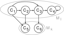
Figure 4: Example of equivalence classes

Let $S\in C_{1}$.

$$\begin{array}[]{rcl}\mu_{\mathcal{R}}(S,M_{l})&=&\mu_{\mathcal{R}}(S,C_{4})+\mu_{\mathcal{R}}(S,C_{5})\\ &&\\ \mu_{\mathcal{R}}(S,C_{4})&=&\tilde{\mu}_{\mathcal{R}}(C_{1},C_{4})\\ &=&\mu_{\mathcal{R}_{1}}(C_{1},C_{4})+\mu_{\mathcal{R}_{1}}(C_{1},C_{2})\tilde{\mu}_{\mathcal{R}}(C_{2},C_{4})\\ &=&\mu_{\mathcal{R}_{1}}(C_{1},C_{4})+\mu_{\mathcal{R}_{1}}(C_{1},C_{2})\mu_{\mathcal{R}_{1}}(C_{2},C_{4})\\ &&\\ \mu_{\mathcal{R}}(S,C_{5})&=&\mu_{\mathcal{R}_{1}}(C_{1},C_{2})\mu_{\mathcal{R}_{1}}(C_{2},C_{5})\\ \end{array}$$

We obtain:

$$\mu_{\mathcal{R}}(S,M_{l})=\mu_{\mathcal{R}_{1}}(C_{1},C_{4})+\mu_{\mathcal{R}_{1}}(C_{1},C_{2})(\mu_{\mathcal{R}_{1}}(C_{2},C_{4})+\mu_{\mathcal{R}_{1}}(C_{2},C_{5}))$$

4 Example: ”H $\leftrightarroweq$ its measurement-based simulation?”

Quantum measurement is universal for quantum computation [Nielsen 2001]. This means that every unitary transformation can be simulated using measurements only. We are interesting in proving with QPAlg that a unitary transformation and its measurement-based simulation behave the same way. We consider the case of the Hadamard transformation $H$.

4.1 Measurement-based simulation of $H$

There exist several models of quantum computation via measurements only. We use the model based on state transfer defined by Perdrix in [Perdrix 2004].

The gate network in figure 5 describes a step of simulation of $H$. This simulation needs an auxiliary qubit initialized in the state $|0\rangle$, it consists in two measurements: one on two qubits with observable $Z\otimes X$ and the other on one qubit with observable $X$. $X$ and $Z$ are Pauli observables. This step simulates $H$ up to a Pauli operator $\sigma$. If $\sigma=I$, $H$ has been simulated, otherwise, a correction must be applied to the result. This correction consists in simulating $\sigma$ (Pauli operators are their proper inverses) in the same way as $H$ has been simulated. The full simulation of $H$ is given by the automaton on figure 6. The states SimulHad, $\boldsymbol{\sigma_{1}}$, $\boldsymbol{\sigma_{2}}$ and $\boldsymbol{\sigma_{3}}$ represent a step of simulation of $H$ and of the Pauli operators.

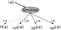
Figure 5: A step of simulation of $H$

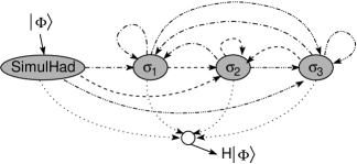
Figure 6: Full simulation of $H$

4.2 Modelling with QPAlg

Unitary transformation of Hadamard.

The process Had applies the Hadamard transformation on a qubit received from gate $g$ and returns this qubit through gate $h$.

$$\mbox{\bf Had}\displaystyle\mathop{=}^{\mathtt{def}}\boldsymbol{[}\ x:\mathtt{Qubit}\boldsymbol{\ }.\ g\ ?x\ H[x]h\ !x\ \mbox{\it nil}\ \boldsymbol{]}$$

Simulation of Hadamard

As for the process Had, the process SimulHad (program 2) begins by receiving a qubit $x$ from gate $g$. Then the Hadamard transformation is simulated in the way described by the automaton shown in figure 6. At the end, the result is in $y$ (and not $x$) which is sent through gate $h$. $\boldsymbol{\sigma}$ is a process simulating a Pauli transformation, the Pauli transformation simulated is specified by the parameter $i$ in $\sigma[i,y]$. The process $\boldsymbol{\sigma}$ is not given, it is organized in a way similar to SimulHad.

$\mbox{\bf SimulHad}\displaystyle\mathop{=}^{\mathtt{def}}$

$\begin{array}[]{ll}\boldsymbol{[}\ y:\mathtt{Qubit},\ i:\mathtt{Nat}\boldsymbol{\ }.&\\ \hskip 20.0pt\boldsymbol{[}\ x:\mathtt{Qubit},\ m,n:\mathtt{Nat}\boldsymbol{\ }.&\\ \hskip 20.0pt\hskip 20.0pt\mbox{\it g}\ ?x&\\ \hskip 20.0pt\hskip 20.0pt(\mbox{\it p}\ ?y\ \mbox{\it end}\parallel\mbox{\it p}\ !0\ \mbox{\it end})\backslash\{\mbox{\it p}\}\ \ ;&\\ \lx@intercol\hskip 20.0pt\hskip 20.0pt(q_{1}\ !Z\otimes X\ [x,y]q_{2}\ !X[x]\ \mbox{\it end}\parallel q_{1}\ ?m\ q_{2}\ ?n\ \mbox{\it end})\backslash\{q_{1},q_{2}\}\ \ ;\hfil\lx@intercol\\ \hskip 20.0pt\hskip 20.0pt(\boldsymbol{[}\\ \hskip 20.0pt\hskip 20.0pt\hskip 20.0pt(m=1\wedge n=1)\rightarrow\mbox{\it r}\ !0\ \mbox{\it end},\\ \hskip 20.0pt\hskip 20.0pt\hskip 20.0pt(m=1\wedge n=-1)\rightarrow\mbox{\it r}\ !1\ \mbox{\it end},&\\ \hskip 20.0pt\hskip 20.0pt\hskip 20.0pt(m=-1\wedge n=1)\rightarrow\mbox{\it r}\ !3\ \mbox{\it end},&\\ \hskip 20.0pt\hskip 20.0pt\hskip 20.0pt(m=-1\wedge n=-1)\rightarrow\mbox{\it r}\ !2\ \mbox{\it end}&\\ \hskip 20.0pt\hskip 20.0pt\boldsymbol{]}\parallel\mbox{\it r}\ ?i\ \mbox{\it end})\backslash\{\mbox{\it r}\}\\ \hskip 20.0pt\boldsymbol{]}\ ;\boldsymbol{\sigma}[i,y]\ ;&\\ \hskip 20.0pth\ !y\ \mbox{\it nil}&\\ \boldsymbol{]}\end{array}$

Program 2 Process for the simulation of $H$

The operational semantics associates with the processes Had and SimulHad (program 2) in empty contexts the process graphs described in figure 7.

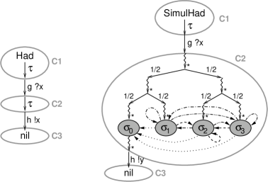
Figure 7: Process graphs of Had and SimulHad in an empty context

4.3 Bisimilarity

To prove that the application of the Hadamard transformation and its measurement-based simulation have the same behavior, we prove that their modellings in QPAlg are bisimilar, i.e. that there exists a bisimulation between Had and SimulHad in empty contexts.

The process graphs of Had and SimulHad in empty contexts are given in figure 7. $C_{1}$, $C_{2}$, $C_{3}$ and $C_{4}$ represents equivalence classes of an equivalence relation $\mathcal{R}$ on process states. This relation is a bisimulation, the main points of this proof are:

• from each process state in $C_{1}$ the transition $g\ ?x\$ can be performed, possibly after several silent transitions

• from each process state in $C_{2}$ the transition $h\ !x\$ or $h\ !y\$ can be performed, possibly after several silent transitions

• when $h\ !x\$ and $h\ !y\$ are performed, the states of $x$ and $y$ are the same

• the probability to reach $C_{3}$ from each state in $C_{2}$ must be the same, which corresponds for any state $S$ in $C_{2}$, to $\mu_{\mathcal{R}}(S,C_{3})=1$

As regards the last point, the computation of the function $\mu_{\mathcal{R}}$ on each state in $C_{2}$ leads to the system of equations in figure 8. We obtain $\forall i\in\{0,\ldots,3\}$, $p_{i}=1$, and then $q_{0}=q_{1}=q_{2}=1$. From any state in the class $C_{2}$, the probability to reach a state in the class $C_{3}$ is 1.

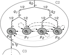
$\begin{array}[]{l}p_{0}=1\\ \forall i\in\{1,2,3\}\ p_{i}=\frac{1}{4}p_{0}+\frac{1}{4}p_{1}+\frac{1}{4}p_{2}+\frac{1}{4}p_{3}\\ q_{1}=\frac{1}{2}p_{0}+\frac{1}{2}p_{1}\\ q_{2}=\frac{1}{2}p_{2}+\frac{1}{2}p_{3}\\ q_{0}=\frac{1}{2}q_{1}+\frac{1}{2}q_{2}\\ \end{array}$

Figure 8: Computation of the probabilities

To conclude, there exists a bisimulation relation between the modelling of the application of Hadamard and the modelling of its measurement-based simulation.

5 Is $\leftrightarroweq$ a congruence?

A natural question about the bisimilarity defined in this section is: is it a congruence? In fact, this question does not make much sense since this relation is defined on process states (process and context) and there exist no composition operators on process states.

There are two possibilities to make it a congruence, either the operators on processes are extended to operators on process states or a congruence on processes is defined from the bisimilarity relation on process states.

We explore the second possibility. A relation $\sim$ on processes is defined: if $P$ and $Q$ are two processes, $P\sim Q\Leftrightarrow\forall C,P/C\leftrightarroweq Q/C$.

Nonetheless, $\sim$ is not a congruence, as shown by the two following examples:

$$\begin{array}[]{rrcl}&H[x]g\ !x\ \mbox{\it nil}&\sim&g\ !x\ \mbox{\it nil}\\ \mbox{but}&H[x]g\ !x\ \mbox{\it nil}+h\ !2\ \mbox{\it nil}&\not\sim&g\ !x\ \mbox{\it nil}+h\ !2\ \mbox{\it nil}\\ &&&\\ &H[x]g\ !x\ \mbox{\it nil}&\sim&g\ !x\ \mbox{\it nil}\oplus_{0.3}g\ !x\ \mbox{\it nil}\\ \mbox{but}&H[x]g\ !x\ \mbox{\it nil}+h\ !2\ \mbox{\it nil}&\not\sim&(g\ !x\ \mbox{\it nil}\oplus_{0.3}g\ !x\ \mbox{\it nil})+h\ !2\ \mbox{\it nil}\end{array}$$

To overcome these problems, probabilistic rooted branching bisimulation and probabilistic rooted branching bisimilarity are defined.

Definition 4

Let $\mathcal{B}$ be an equivalence relation. $\mathcal{B}$ is a probabilistic rooted branching bisimulation if and only if:

• if $S\mathcal{B}T$ and $S\xrightarrow{\ a\ }S^{\prime}$ ($a=g\ !v\$ or $g\ ?v\$ or $\tau$) then $T\xrightarrow{\ a\ }T^{\prime}$ with $S^{\prime}\leftrightarroweq T^{\prime}$

• if $S\mathcal{B}T$ and $S\mbox{$\displaystyle\ \mathop{-\!-\longrightarrow}^{g\ !x\ }\ $}S^{\prime}$,then $T\mbox{$\displaystyle\ \mathop{-\!-\longrightarrow}^{g\ !y\ }\ $}T^{\prime}$ with $\rho_{x}^{S}=\rho_{y}^{T}$ and $S^{\prime}\leftrightarroweq T^{\prime}$

• if $S\mathcal{B}T$ and $S\mbox{$\displaystyle\ \mathop{-\!-\longrightarrow}^{g\ ?x\ }\ $}S^{\prime}$, then $T\mbox{$\displaystyle\ \mathop{-\!-\longrightarrow}^{g\ ?y\ }\ $}T^{\prime}$ with $\rho_{x}^{S^{\prime}}=\rho_{y}^{T^{\prime}}$ and $S^{\prime}\leftrightarroweq T^{\prime}$

• if $S\mathcal{B}T$ and $S\longrightarrow_{p}S^{\prime}$, then $T\longrightarrow_{q}T^{\prime}$ with $S^{\prime}\mathcal{B}T^{\prime}$

• if $S\mathcal{B}T$ then $\mu_{\leftrightarroweq}(S,M)=\mu_{\leftrightarroweq}(T,M),\ \forall M\in\mathcal{S}/\leftrightarroweq$

Definition 5

Two process states $S$ and $T$ are probabilistic rooted branching bisimilar, denoted $S\leftrightarroweq_{r}T$, if and only if there is a probabilistic branching bisimulation $\mathcal{B}$ such that $S\mathcal{B}T$.

Proposition 2

$\leftrightarroweq_{r}$ is an equivalence relation.

Proof.  From the fact that $\leftrightarroweq$ is an equivalence relation. $\diamond$

Note.  For all $S$, $T$ in $\mathcal{S}$: $S\leftrightarroweq_{r}T$ implies $S\leftrightarroweq T$

Definition 6

Let $P$ and $Q$ be two processes.

$$P\sim Q\Leftrightarrow\forall C,P/C\leftrightarroweq_{r}Q/C$$

Proposition 3

$\sim$ is an equivalence relation and is preserved by variable declaration, action prefix, nondeterministic choice, probabilistic choice, conditional choice and restriction.

Proof.  Since $\leftrightarroweq_{r}$ is an equivalence relation, it is easy to see that $\sim$ is also an equivalence relation.

Let $P$, $Q$ be processes such that $P\sim Q$, that is to say $\forall C,P/C\leftrightarroweq_{r}Q/C$.

Action prefix. Let $a$ be an action. The question is: are $aP/C$ and $aQ/C$ probabilistically rooted branching bisimilar for all context $C$?

If $C$ is probabilistically stable: $aP/C\xrightarrow{\ a\ }P/C^{\prime}$ and $aQ/C\xrightarrow{\ a\ }Q/C^{\prime}$. $P/C^{\prime}\leftrightarroweq_{r}Q/C^{\prime}$ implies $P/C^{\prime}\leftrightarroweq Q/C^{\prime}$. $\mathcal{B}=\{(aP/C,aQ/C)\}$ is a probabilistic rooted branching bisimulation.

If $C=\mathop{\boxplus}_{p_{i}}C_{i}$: for all $i$, $aP/C\longrightarrow_{p_{i}}aP/C_{i}$ and $aQ/C\longrightarrow_{p_{i}}aQ/C_{i}$. From the previous case, $\forall\ i$: $aP/C_{i}\leftrightarroweq_{r}aQ/C_{i}$, we deduce $aP/C\leftrightarroweq_{r}aQ/C$.

Nondeterminism. Let $R$ be a process. The question is: are $P+R/C$ and $Q+R/C$ probabilistic rooted branching bisimilar, for all context $C$?

If $C$ is probabilistically stable: If $P+R/C\dashrightarrow P^{\prime}/C_{P}$ then, as $P/C\leftrightarroweq_{r}Q/C$, there exists $Q^{\prime}/C_{Q}$ such that $Q+R/C\dashrightarrow Q^{\prime}/C_{Q}$ and $P^{\prime}/C_{P}\leftrightarroweq Q^{\prime}/C_{Q}$. Otherwise $P+R/C\dashrightarrow R^{\prime}/C^{\prime\prime}$ then, $Q+R/C\dashrightarrow R^{\prime}/C^{\prime\prime}$ and $R^{\prime}/C^{\prime\prime}\leftrightarroweq R^{\prime}/C^{\prime\prime}$.

If $C$ is not probabilistically stable, we reduce the problem to the previous point after a probabilistic transition.

The other points are similar to those developed. $\diamond$

We conclude that $\sim$ is preserved by all operators except $\parallel$, as shown by the following example: $(g\ !2\ h\ !3\ \mbox{\it nil}\parallel g\ ?x\ h\ ?x\ \mbox{\it nil})\backslash\{g,h\}\ \sim(h\ !3\ \mbox{\it nil}\parallel h\ ?x\ \mbox{\it nil})\backslash\{h\}\$, nonetheless, $(g\ !2\ h\ !3\ \mbox{\it nil}\parallel g\ ?x\ h\ ?x\ \mbox{\it nil})\backslash\{g,h\}\ \parallel k\ !x\ \mbox{\it nil}\not\sim(h\ !3\ \mbox{\it nil}\parallel h\ ?x\ \mbox{\it nil})\backslash\{h\}\ \parallel k\ !x\ \mbox{\it nil}$. The left process can send $2$ or $3$ through gate $k$ whereas the right process can only send $3$.

This problem could be overcome by restricting processes in parallel not to use the same variable names. This is done in CQP [Nagarajan and Gay 2004] and can be justified by the fact that variables cannot be at two places at the same time. However, because of entanglement in the quantum state, this does not solve the whole problem:

$$\begin{array}[]{rcl}M_{std,1}[x]\mbox{\it nil}&\sim&I[x](0\mbox{\it nil}\oplus_{0.5}1\mbox{\it nil})\\ M_{std,1}[x]\mbox{\it nil}\parallel g\ !y\ \mbox{\it nil}&\not\sim&(I[x](0\mbox{\it nil}\oplus_{0.5}1\mbox{\it nil}))\parallel g\ !y\ \mbox{\it nil}\end{array}$$

In a configuration where the state of $x$ and $y$ is $\frac{1}{\sqrt{2}}(|00\rangle+|11\rangle)$ (EPR state), the left process can send the qubit $y$ in the mixed state $\{0.5:|0\rangle,0.5:|1\rangle\}$ through gate $g$ if $M_{std,1}[x]$ has not been applied, or in the states $|0\rangle$ or $|1\rangle$ if the measurement has been applied, whereas the right process can only send $y$ in the state $\{0.5:|0\rangle,0.5:|1\rangle\}$.

6 Conclusion

This paper has presented a process algebra for quantum programming which can describe both classical and quantum programming, and their cooperation. This language has an operational semantics, one of its peculiarities is the introduction of probabilistic transitions, due to quantum measurement and to the operator of probabilistic choice.

Then a semantical equivalence relation on process states has been defined. This equivalence is a bisimulation which identifies processes associated with process graphs having the same branching structure. From this bisimulation, an equivalence relation on processes has been defined. This relation is preserved by all the operators of the process algebra except parallel composition. This is a first step toward the verification of quantum cryptographic protocols.

Several extensions are possible. As already mentioned, we could define a congruence on process states from the bisimulation defined here by extending the operators on processes to operators on process states. Another possible extension is the definition of a type system to verify statically properties such as the no-cloning theorem (quantum variables cannot be copied).

Appendix A The quantum process algebra

A.1 Syntax

Expressions
qexp	$::=$	qvar $\boldsymbol{\otimes}$ qexp $|$ qvar
nexp	$::=$	nfact $\boldsymbol{+}$ nexp $|$ nfact $\boldsymbol{-}$ nexp $|$ nfact
nfact	$::=$	nterm $\boldsymbol{\times}$ nfact $|$ nterm $\boldsymbol{\div}$ nfact $|$ nterm
nterm	$::=$	nvar $|$ nval $|$ transf_admissible $\boldsymbol{[}$ qexp $\boldsymbol{]}$
	$|$	$\boldsymbol{(}$ nexp $\boldsymbol{)}$ $|$ $\boldsymbol{-}$nterm
Actions
communication	$::=$	gate ! variable $|$ gate ! nexp
	$|$	gate ? variable
action	$::=$	communication $|$ nexp
Processes
type	$::=$	$\boldsymbol{\mathtt{Nat}}\ |\ \boldsymbol{\mathtt{Qubit}}$
variable_decl	$::=$	variable $\boldsymbol{:}$ type $\{\boldsymbol{,}$ variable $\boldsymbol{:}$ type $\}^{*}$
process	$::=$	nil
	$|$	name $\{\boldsymbol{[}$ variable_list $\boldsymbol{]}\}$
	$|$	param_decl $\boldsymbol{\bullet}$ process $\boldsymbol{[}$ variable_list $\boldsymbol{]}$
	$|$	$\boldsymbol{\boldsymbol{[}\ }$ variable_decl . process $\boldsymbol{\ \boldsymbol{]}}$
	$|$	action $\boldsymbol{missing}$ process
	$|$	process $\boldsymbol{\parallel}$ process
	$|$	process $\boldsymbol{+}$ process
	$|$	$\boldsymbol{\boldsymbol{[}\ }$ condition $\boldsymbol{\rightarrow}$ process $\{\boldsymbol{,}$ condition $\boldsymbol{\rightarrow}$ process $\}^{*}\boldsymbol{\ \boldsymbol{]}}$
	$|$	process $\{\boldsymbol{\oplus}_{\mbox{probability}}$ process$\}^{+}$
	$|$	process $\boldsymbol{\backslash}\boldsymbol{\{}$ gate_list $\boldsymbol{\}}$
param_decl	$::=$	$\boldsymbol{\boldsymbol{[}\ }$ variable_decl $\boldsymbol{\ \boldsymbol{]}}$
process_decl	$::=$	name $\boldsymbol{\displaystyle\mathop{=}^{\mathtt{def}}}$ process $|$ nom $\boldsymbol{\displaystyle\mathop{=}^{\mathtt{def}}}$ param_decl $\boldsymbol{\bullet}$ process

A.2 Main inference rules of the semantics

The semantics is specified with inference rules which give the evolution of the states of processes. There are five kinds of transitions:

• transitions for evaluating expressions: $\longrightarrow_{v}$ and $\longrightarrow_{e}$

• action transitions: $\displaystyle\ \mathop{-\!-\longrightarrow}^{\alpha}\$ where $\alpha$ is $g\ !x\$ or $g\ ?x\$;

• silent transitions: $\displaystyle\ \mathop{\longrightarrow}^{\tau}\$, for internal transition;

• probabilistic transitions: $\longrightarrow_{p}$, where $p$ is a probability.

In the following, $P,Q,P^{\prime},Q^{\prime},P_{i}$ and $P_{i}^{\prime}$ are processes, $C$, $C^{\prime}$ and $C_{i}$ are contexts, $\alpha$ is an action, $g$ is a communication gate, $v$ is a value, $x$ is a variable, and $c_{j}$ is a condition.

Expressions

$$\frac{}{x/<s,q=\rho,f>\longrightarrow_{v}f(x)/<s,q=\rho,f>}\hskip 20.0ptx\in\mbox{dom($f$)}$$ (1)

$$\frac{}{A[x_{1}\otimes\ldots\otimes x_{n}]/C\longrightarrow_{v}y/\mathop{\boxplus}_{p_{i}}C_{i}}$$ (2)

avec

• $A=\{A_{\tau_{1}},\ldots,A_{\tau_{n}}\}$, admissible transformation

• $y$, fresh variable name

• $C=<e.s,q=\rho,f>$

• $C_{i}=<(\{y:\mathtt{Nat}\}\cup e).s,q=\rho_{i},f\cup\{y\mapsto\tau_{i}\}>$

• $x_{1},\ldots,x_{n}\in q$

• $p_{i}=Tr(\mathcal{T}_{A_{\tau_{i}}}(\rho))$ and $\rho_{i}=\frac{1}{p_{i}}\mathcal{T}_{A_{\tau_{i}}}(\rho)$

Evaluation contexts

$E[\ ]$ is an evaluation context of an expression, it is an expression in which a sub-expression has been replaced by $[\ ]$. Similarly, $F[\ ]$ is an evaluation context of a process.

$$\frac{e/C\longrightarrow_{v}e^{\prime}/C^{\prime}}{E[e]/C\longrightarrow_{e}E[e^{\prime}]/C^{\prime}}$$ (3)

$$\frac{e/C\longrightarrow_{e}e^{\prime}/C^{\prime}}{F[e]/C\mbox{$\displaystyle\ \mathop{\longrightarrow}^{\tau}\ $}F[e^{\prime}]/C^{\prime}}$$ (4)

Action Prefix

Communication.

$$\frac{}{g\ !v\ P/C\mbox{$\displaystyle\ \mathop{-\!-\longrightarrow}^{g\ !v\ }\ $}P/C}\hskip 20.0ptv\in I\!\!N$$ (5)

$$\frac{}{g\ !x\ P/C\mbox{$\displaystyle\ \mathop{-\!-\longrightarrow}^{g\ !x\ }\ $}P/C}\hskip 20.0ptC=<s,q=\rho,f>\mbox{ and }x\in q$$ (6)

For all $v\in I\!\!N$:

$$\frac{}{g\ ?x\ P/C\mbox{$\displaystyle\ \mathop{-\!-\longrightarrow}^{g\ ?v\ }\ $}P/C^{\prime}}$$ (7)

with $C=<s,q=\rho,f>$, $C^{\prime}=<s,q=\rho,f\cup\{x\mapsto v\}>$ and $(x,\mathtt{Nat})\in s$

For all density matrix $\nu$ of dimension $2$:

$$\frac{}{g\ ?x\ P/C\mbox{$\displaystyle\ \mathop{-\!-\longrightarrow}^{g\ ?x\ }\ $}P/C^{\prime}}$$ (8)

with

• $C=<s,q=\rho,f>$, $C^{\prime}=<s,x.q=\nu\otimes\rho,f>$

• $(x,\mathtt{Qubit})\in s$ and $x\not\in q$

Expression.

$$\frac{}{vP/C\mbox{$\displaystyle\ \mathop{\longrightarrow}^{\tau}\ $}P/C}\hskip 20.0ptv\in I\!\!N$$ (9)

Probabilities

$$\frac{}{P/\mathop{\boxplus}_{p_{j}}C_{j}\longrightarrow_{p_{i}}P/C_{i}}\hskip 20.0pt\sum_{j}p_{j}=1$$ (10)

$$\frac{}{\bigoplus_{p_{j}}P_{j}/C\longrightarrow_{p_{i}}P_{i}/C}\hskip 20.0pt\sum_{j}p_{j}=1$$ (11)

Nondeterministic choice

$$\frac{P/C\dashrightarrow P^{\prime}/C^{\prime}}{P+Q/C\dashrightarrow P^{\prime}/C^{\prime}}\hskip 20.0ptP\downarrow,Q\downarrow$$ (12)

where $\dashrightarrow$ represents any transition.

$$\frac{P/C\longrightarrow_{p}P^{\prime}/C^{\prime}}{P+Q/C\longrightarrow_{p}P^{\prime}+Q/C^{\prime}}\hskip 20.0ptQ\downarrow$$ (13)

$$\frac{P/C\longrightarrow_{p}P^{\prime}/C^{\prime}\hskip 20.0ptQ/C\longrightarrow_{q}Q^{\prime}/C^{\prime\prime}}{P+Q/C\longrightarrow_{pq}P^{\prime}+Q^{\prime}/C}$$ (14)

Parallel composition

In the rules for parallel composition, $C$, $C_{P}$ and $C_{Q}$ are defined as:

• $C=<(s_{P}\parallel s_{Q}).s,q=\rho,f>$

• $C_{P}=<s_{P}|s,q=\rho,f>$

• $C_{Q}=<s_{Q}|s,q=\rho,f>$

In the definition of $C$, the operator $\parallel$ permits to build a cactus stack (see paragraph 2.1). In the cactus stack $(s_{P}\parallel s_{Q}).s$ of the process $P\parallel Q$, the names in $s$ correspond to variables shared by $P$ and $Q$ whereas the names in $s_{P}$ (resp. $s_{Q}$) correspond to variables declared in $P$ (resp. $Q$).

$$\frac{P/C_{P}\mbox{$\displaystyle\ \mathop{-\!-\longrightarrow}^{\alpha}\ $}P^{\prime}/C_{P}^{\prime}}{P\parallel Q/C\mbox{$\displaystyle\ \mathop{-\!-\longrightarrow}^{\alpha}\ $}P^{\prime}\parallel Q/C^{\prime}}\hskip 20.0ptP\downarrow,Q\downarrow$$ (15)

where

• If $C_{P}^{\prime}=<s^{\prime},q^{\prime}=\rho^{\prime},f^{\prime}>$ then $C^{\prime}=<(s_{P}^{\prime}\parallel s_{Q}).s,q^{\prime}=\rho^{\prime},f^{\prime}>$ with $s_{P}^{\prime}$ such that $s^{\prime}=s_{P}^{\prime}|s$ ($P$ can neither add to nor remove variables from $s$)

• If $C_{P}^{\prime}=\mathop{\boxplus}_{p_{i}}\!\!<s_{i}^{\prime},q_{i}^{\prime}=\rho_{i}^{\prime},f_{i}^{\prime}>$ then $C^{\prime}=\mathop{\boxplus}_{p_{i}}\!\!<({s_{P}}_{i}^{\prime}\parallel s_{Q}).s,q_{i}^{\prime}=\rho_{i}^{\prime},f_{i}^{\prime}>$ with ${s_{P}}_{i}^{\prime}$ such that $s_{i}^{\prime}={s_{P}}_{i}^{\prime}|s$

$$\frac{P/C_{P}\mbox{$\displaystyle\ \mathop{-\!-\longrightarrow}^{g\ !v\ }\ $}P^{\prime}/C_{P}^{\prime}\hskip 20.0ptQ/C_{Q}\mbox{$\displaystyle\ \mathop{-\!-\longrightarrow}^{g\ ?v\ }\ $}Q^{\prime}/C_{Q}^{\prime}}{P\parallel Q/C\mbox{$\displaystyle\ \mathop{\longrightarrow}^{\tau}\ $}P^{\prime}\parallel Q^{\prime}/C^{\prime}}\hskip 20.0ptP\downarrow,Q\downarrow$$ (16)

where $v\in I\!\!N$, $C_{Q}^{\prime}=<s^{\prime},q^{\prime}=\rho^{\prime},f^{\prime}>$, and $C^{\prime}=<(s_{P}\parallel s_{Q}).s,q=\rho,f^{\prime}>$

$$\frac{P/C_{P}\mbox{$\displaystyle\ \mathop{-\!-\longrightarrow}^{g\ !v\ }\ $}P^{\prime}/C_{P}^{\prime}\hskip 20.0ptQ/C_{Q}\mbox{$\displaystyle\ \mathop{-\!-\longrightarrow}^{g\ ?y\ }\ $}Q^{\prime}/C_{Q}^{\prime}}{P\parallel Q/C\mbox{$\displaystyle\ \mathop{\longrightarrow}^{\tau}\ $}P^{\prime}\parallel Q^{\prime}/C^{\prime}}\hskip 20.0ptP\downarrow,Q\downarrow$$ (17)

where

• $(x,\mathtt{Qubit})\in s\cup s_{Q}$, $x\not\in q$, $v\in\{0,1\}$

• $C^{\prime}=<(s_{P}\parallel s_{Q}).s,x.q=|v\rangle\langle v|\otimes\rho,f>$

$$\frac{P/C_{P}\mbox{$\displaystyle\ \mathop{-\!-\longrightarrow}^{g\ !x\ }\ $}P^{\prime}/C_{P}^{\prime}\hskip 20.0ptQ/C_{Q}\mbox{$\displaystyle\ \mathop{-\!-\longrightarrow}^{g\ ?y\ }\ $}Q^{\prime}/C_{Q}^{\prime}}{P\parallel Q/C\mbox{$\displaystyle\ \mathop{\longrightarrow}^{\tau}\ $}P^{\prime}\parallel Q^{\prime}/C^{\prime}}\hskip 20.0ptP\downarrow,Q\downarrow$$ (18)

where

• $(x,\mathtt{Qubit})\in s\cup s_{P}$, $x\in q$

• $(y,\mathtt{Qubit})\in s\cup s_{Q}$, $y\not\in q$

• $C^{\prime}=<((s_{P}\parallel s_{Q}).s)\backslash\{x\},q[x\leftarrow y]=\rho,f>$

$$\frac{P/C_{P}\longrightarrow_{p}P^{\prime}/C_{P}^{\prime}}{P\parallel Q/C\longrightarrow_{p}P^{\prime}\parallel Q/C}\hskip 20.0ptQ\downarrow$$ (19)

$$\frac{P/C_{P}\longrightarrow_{p}P^{\prime}/C_{P}^{\prime}\hskip 20.0ptQ/C_{Q}\longrightarrow_{q}Q^{\prime}/C_{Q}^{\prime}}{P\parallel Q/C\longrightarrow_{pq}P^{\prime}\parallel Q^{\prime}/C}$$ (20)

References

• [Andova 1999] Andova, S. (1999) Process algebra with probabilistic choice. Lecture Notes in Computer Science, 1601:111–129.
• [Arrighi and Dowek 2004] Arrighi, P. and Dowek, G. (2004) Operational semantics for formal tensorial calculus. In P. Selinger, editor, Proceedings of the 2nd International Workshop on Quantum Programming Languages, pages 21 – 38.
• [Bennett et al. 1993] Bennett, C. H., Brassard, G., Crépeau, C., Jozsa, R., Peres, A., and Wootters, W. (1993) Teleporting an unknown quantum state via dual classical and EPR channels. Physical Review Letters, 70:1895–1899.
• [Bolognesi and Brinksma 1987] Bolognesi, T. and Brinksma, E. (1987) Introduction to the ISO specification language LOTOS. Computer Networks and ISDN Systems, 14(1):25–59.
• [Cazorla et al. 2001] Cazorla, D., Cuartero, F., Valero, V., and Pelayo, F. L. (2001) A process algebra for probabilistic and nondeterministic processes. Information Processing Letters, 80(1):15–23.
• [Cazorla et al. 2003] Cazorla, D., Cuartero, F., Valero, V., Pelayo, F. L, and Pardo, J. (2003) Algebraic theory of probabilistic and nondeterministic processes. The Journal of Logic and Algebraic Programming, 55(1–2):57–103.
• [Fokkink 2000] Fokkink, W. (2000) Introduction to Process Algebra. Springer.
• [Lalire and Jorrand 2004] Lalire, M. and Jorrand, P. (2004) A process algebraic approach to concurrent and distributed quantum computation: operational semantics. In P. Selinger, editor, Proceedings of the 2nd International Workshop on Quantum Programming Languages, pages 109 – 126.
• [Milner 1989] Milner, R. (1989) Communication and Concurrency. Prentice-Hall, London.
• [Nagarajan and Gay 2004] Nagarajan, R. and Gay, S. (2004) Communicating quantum processes. In P. Selinger, editor, Proceedings of the 2nd International Workshop on Quantum Programming Languages, pages 91 – 107.
• [Nielsen 2001] Nielsen, M. (2001) Universal quantum computation using only projective measurement, quantum memory and preparation of the 0 state. Los Alamos e-print arXiv.
• [Nielsen and Chuang 2000] Nielsen, M. A. and Chuang, I. L. (2000) Quantum Computation and Quantum Information. Cambridge University Press.
• [Ömer 2000] Ömer, B. (2000) Quantum programming in QCL. Master’s thesis, Institute of Information Systems, Technical University of Vienna.
• [Perdrix 2004] Perdrix, S. (2004) State transfer instead of teleportation in measurement-based quantum computation. Los Alamos e-print arXiv.
• [Roscoe 1998] Roscoe, A. W. (1998) The theory and practice of concurrency. Prentice-Hall.
• [Selinger 2004] Selinger, P. (2004) Toward a quantum programming language. Mathematical Structures in Computer Science, 14(4):525 – 586.
• [van Glabbeek 1993] van Glabbeek, R. (1993) The linear time – branching time spectrum ii: the semantics of sequential systems with silent moves. In E. Best, editor, Proceedings of the 4th Conference on Concurrency Theory (CONCUR’93), pages 66–81, Hildesheim. LNCS 715. Springer.
• [van Tonder 2003] Van Tonder, A. (2003) A lambda calculus for quantum computation. Los Alamos e-print arXiv.
• [Zuliani 2001] Zuliani, P. (2001) Quantum Programming. PhD thesis, St Cross College, University of Oxford.