Quantum baker maps with controlled-NOT coupling

Abstract

The characteristic stretching and squeezing of chaotic motion is linearized within the finite number of phase space domains which subdivide a classical baker map. Tensor products of such maps are also chaotic, but a more interesting generalized baker map arises if the stacking orders for the factor maps are allowed to interact. These maps are readily quantized, in such a way that the stacking interaction is entirely attributed to primary qubits in each map, if each j’th subsystem has Hilbert space dimension $D_{j}=2^{n_{j}}$. We here study the particular example of two baker maps that interact via a controlled-not interaction, which is a universal gate for quantum computation. Numerical evidence indicates that the control subspace becomes an ideal Markovian environment for the target map in the limit of large Hilbert space dimension.

I Introduction

The baker map displays the essential features of classically chaotic motion in such a simplified form as to be almost a caricature. It may be described as a space-filling horseshoe map that linearizes the hyperbolic motion. Thus, essentially chaotic motion is exhibited, which can be followed through very simple computations. The binary symbolic dynamics propagates vertical strips in the unit square onto horizontal strips. The vertical and horizontal rectangles are narrower, for longer binary codes, so that the primary digit specifies a half-square. Hence this digit is responsible for a coarse-grained description of the motion. The way in which horizontal strips are piled up by the mapping is also determined by the primary binary digit.

The various quantization schemes that have been proposed for the baker map generally respect the main division of the square into a pair of vertical rectangles, which split the position states into Hilbert subspaces. These are mapped respectively onto a pair of momentum subspaces according to the primary binary digit. The discrete and finite nature of the Hilbert space prevents the association of longer codes to ever thinner strips SAV . Thus, to some extent, the primary digit is even more important in quantum mechanics. Initially, it may have seemed that the introduction of binary symbols to describe evolving quantum systems could only serve as an artificial prop for the study of the semiclassical limit. However, the growing interest in quantum computation has brought the binary structure to the fore. Schack noted that the quantum baker could be efficiently realized in terms of quantum gates schack98 . A three qubit Nuclear Magnetic Resonance experiment was proposed brun99 and then implemented (with some simplifications) weinstein02 . In this context, the quantum baker map has reemerged as an ideal simplified model. Schack and Caves SchackCaves have indeed developed an entire class of quantum baker maps, based on the $2^{N}$-dimensional Hilbert space of $N$ qubits, which include the original quantizations of Balazs and Voros BalazsVoros and Saraceno Saraceno as special cases. While incorporating the qubit structure and hence a Hilbert space of $D=2^{N}$ dimensions, we here adopt the Balazs-Voros-Saraceno map throughout, since this singles out the primary bit most clearly.

The object of our study is the coupling of quantum baker maps, initially restricted to a pair of maps. Clearly, the higher dimensional product-map of classical baker maps is also chaotic, in spite of possible added symmetries. The minimal coupling that can be meaningfully addressed relies exclusively on the primary binary digit. Thus, each baker map is only sensitive to the most coarse-grained information available about the state of the other map. In other words, one can investigate the class of coupled baker maps that interact through the order in which the pair of horizontal rectangles are piled up. Once these coupled maps are quantized, this corresponds to an interaction among only the primary qubits.

It is important at this stage to distinguish two alternative forms of classical-quantum correspondence for individual baker maps. In the original quantizations BalazsVoros ; Saraceno , the classical phase space is two-dimensional and it is the chaotic motion in this two-dimensional torus that corresponds to the quantum level repulsion, in keeping with the spectra of random matrices Bohigas . If the quantization is chosen with a value of Planck’s constant such that the Hilbert space has exactly $2^{N}$ states, then it is possible to reinterpret the quantum system to be the tensor product of $N$ two-level systems. This would correspond to a hypercube in a $2N$-dimensional phase space, but it would be stretching it to ascribe a classical correspondence to this quintessentially quantum system. We shall here keep to the original quantization schemes and, hence, interpret each quantum baker map as corresponding to a classical two-dimensional phase space, so that the coupling of two baker maps corresponds to a four-dimensional phase space. The four possible combinations of primary binary digits –$(0,0),(0,1),(1,0),(1,1)$– then correspond to four squares in the classical position space $(q_{1},q_{2})$ and hence to four parallelepipeds in the unit 4-cube $(q_{1},q_{2},p_{1},p_{2})$ in which the classical motion is defined.

Perhaps the simplest choice for coupling two classical bakers is a simple switch of the piling: Each map stacks in accordance to the other’s primary digit. Obviously, there is then no change if their digits coincide, but, otherwise, both maps invert their piling. This is analogous to a mutual spin flip for the principal qubits of the quantized “switch baker map”. Notice that this interaction does not break the exchange symmetry of the product map.

As a direct model for (quantum) computing, we here concentrate on the “controlled-not baker map”. In this unsymmetric case, the control map evolves just as an ordinary baker map, while it determines the stacking of the target map. The latter piles its rectangles as a normal baker when the primary digit of the control map is zero, but this is switched when the control digit is one. It is well known that the controlled-not gate is a basic element of quantum computing Nielsen . The present may be considered as an interesting example of a system where only a singe element of a higher dimensional Hilbert space determines a qubit. This has been advocated as possibly beneficial for the stabilization of quantum computation against decoherence OM .

It is possible to study the evolution of the entanglement of the various qubits resulting from the iteration of an individual quantum baker map ScottCaves . In the case of coupled baker maps, we can interpret the primary bit of each component baker map as implicated in quantum computation, while the remaining qubits in each map model the local environment, leading to a loss of quantum coherence. Alternatively, we here consider a second baker map as a model for the environment coupled to the map that is singled out as the open quantum system.

The presentation of the class of minimally coupled maps is preceeded by a brief review of the ordinary two-dimensional baker map and its quantization in section 2. Section 3 then presents the coupled maps and their quantization with special emphasis on the controlled-not baker map. The evolution of bipartite entanglement of a product pure state is studied in section 4 by considering the control and the target of the controlled-not baker as the separate subsystems. The asymmetric nature of this interaction suggests that this should be an ideal Markovian system, in the appropriate limit, as far as the target is concerned. This is verified by the evolution of the linear entropy. Our results are discussed in section 5.

II Review of classical and quantum baker maps

In this section we present the well known classical and quantum ingredients of baker maps. However, the alternative pilings, which are usually equivalent, need to be made explicit when different maps are coupled.

The classical baker transformation is an area preserving, piecewise–linear map, ${\bf b}:(p_{0},q_{0})\rightarrow(p_{1},q_{1})$ of the unit square (periodic boundary conditions are assumed) defined as

$$p_{1}=\frac{1}{2}(p_{0}+\epsilon_{0})~{},~{}~{}~{}q_{1}=2q_{0}-\epsilon_{0}~{};$$ (1)

where $\epsilon_{0}=[2q_{0}]$, the integer part of $2q_{0}$. This map is known to be uniformly hyperbolic, the stability exponent for orbits of period $L$ being $L\log 2$. Moreover it admits a useful description in terms of a complete symbolic dynamics. A one to one correspondence between phase space coordinates and binary sequences,

$$(p,q)\leftrightarrow\ldots\epsilon_{-2}\epsilon_{-1}\cdot\epsilon_{0}\epsilon_{1}\epsilon_{2}\ldots~{}~{}~{},~{}\epsilon_{i}=0,1~{},$$ (2)

can be constructed in such a way that the action of the map is conjugated to a shift map. The symbols are assigned as follows: $\epsilon_{i}$ is set to zero (one) when the $i$–th iteration of $(p,q)$ falls to the left (right) of the line $q=1/2$, i.e. $[2q_{i}]=\epsilon_{i}$. Reciprocally, given an itinerary

$$\ldots\epsilon_{-2}\epsilon_{-1}\cdot\epsilon_{0}\epsilon_{1}\epsilon_{2}\ldots,$$ (3)

the related phase point is obtained through the specially simple binary expansions

$$q=\sum_{i=0}^{\infty}\frac{\epsilon_{i}}{2^{i+1}}~{},~{}~{}~{}p=\sum_{i=1}^{\infty}\frac{\epsilon_{-i}}{2^{i}}~{}.$$ (4)

Once the dynamics has been mapped to a shift on binary sequences it is very easy to analyze the dynamical features of the map. In particular, periodic points are associated to infinite repetitions of finite sequences of symbols.

Due to its piecewise linear nature, the baker map admits a (mixed) generating function which is a piecewise bilinear form,

$$W_{\epsilon_{0}}(p_{1},q_{0})=2p_{1}q_{0}-\epsilon_{0}p_{1}-\epsilon_{0}q_{0}~{},~{}~{}~{}\epsilon_{0}=0,1~{}.$$ (5)

It is not defined on the whole space $(p_{1},q_{0})$ but on the classically allowed domains

$$R_{0}=[0,1/2]\otimes[0,1/2]~{}~{}~{}\mbox{and}~{}~{}~{}R_{1}=[1/2,1]\otimes[1/2,1]~{}.$$ (6)

Though the above generating function will be the starting point for quantization, it must be remembered that it only provides an implicit formula for each iteration of the classical baker map.

With respect to the quantum map, we will follow the original quantization of Balazs and Voros BalazsVoros , as later modified by Saraceno Saraceno to preserve in the quantum map all the symmetries of its classical counterpart. In the mixed representation the baker’s propagator can be written as a $D\times D$ block–matrix ($D$ even):

$$\langle p_{m}|{\widehat{B}}_{D}|q_{n}\rangle=\left(\begin{array}[]{cc}G_{D/2}&0\\ 0&G_{D/2}\end{array}\right)~{},$$ (7)

where position and momentum eigenvalues run on a discrete mesh with step $1/D=h$ ($h$ = Planck’s constant), so that

$$q_{n}=(n+1/2)/D~{},~{}~{}~{}p_{m}=(m+1/2)/D~{},~{}~{}~{}0\leq n,m\leq D-1~{};$$ (8)

and $G_{D}$ is the antiperiodic Fourier matrix, which transforms from the $q$ to the $p$ basis,

$$G_{D}=\langle p_{m}|q_{n}\rangle=(1/\sqrt{D})e^{-2\pi iDp_{m}q_{n}}~{}.$$ (9)

It will be useful to consider this matrix as the position representation of the Fourier operator $\widehat{G}_{D}$, such that $\widehat{G}_{D}|p_{n}\rangle=|q_{n}\rangle$ .

The mixed propagator (7) has the standard structure of quantized linear symplectic maps OZS ,

$$\langle p_{m}|{\widehat{B}}_{D}|q_{n}\rangle=\left\{\begin{array}[]{cl}\sqrt{2/D}\,e^{-i2\pi DW_{0}(p_{m},q_{n})}&\mbox{if}~{}~{}(p_{m},q_{n})\,\in\,R_{0}\\ \sqrt{2/D}\,e^{-i2\pi DW_{1}(p_{m},q_{n})}&\mbox{if}~{}~{}(p_{m},q_{n})\,\in\,R_{1}\\ 0&\mbox{otherwise}~{}.\end{array}\right.$$ (10)

In this quantization, only those transitions are allowed that respect the rule $[2p_{m}]=[2q_{n}]$, a reflection of the classical shift property.

To be able to iterate the quantum baker map, the state must be brought back to the position representation. This is achieved by an inverse Fourier transform, so that the matrix (7) is multiplied by $G_{D}^{-1}$.

Following Schack and Caves SchackCaves , we can reinterpret this quantum map as the evolution of $N$ qubits if the dimension of the Hilbert space satisfies $D=2^{N}$. Then the position states can be defined as product states for the qubits in the basis,

$$|q_{n}\rangle=|\epsilon_{1}\rangle\otimes|\epsilon_{2}\rangle\otimes...|\epsilon_{N}\rangle,$$ (11)

where $n$ has the binary expansion

$$n=\epsilon_{1}...\epsilon_{N}=\sum_{j=1}^{N}\epsilon_{j}2^{N-j}$$ (12)

and $q_{n}=(n+1/2)/D=0\cdot\epsilon_{1}...\epsilon_{N}1$. The connection with the classical baker map is specified by the symbolic dynamics. Finite segments of the bi-infinite strings (3) that determine points in the unit square are made to correspond to orthogonal quantum states. Half of the position states lie in either of the two rectangles, $R_{0}$, or $R_{1}$ defined in (6), which correspond respectively to $0$, or $1$ eigenstates of the principal qubit.

The full unitary operator for the quantum baker can be written explicitly as

$${\widehat{B}}_{D}={\widehat{G}}_{D}[{\hat{1}}_{2}\otimes{\widehat{G}}^{-1}_{D/2}],$$ (13)

where ${\hat{1}}_{2}$ is the unit operator for the first qubit and ${\widehat{G}}^{-1}_{D/2}$ is the inverse Fourier operator on the remaining qubits. The operator in the square brackets preserves the first qubit, while evolving separately the remaining qubits, within each domain $R_{\epsilon_{1}}$. It is the final Fourier operator that mixes the principal qubit in with the rest, because it acts globally on the states in both domains. This step is not explicit in the mixed representation (7).

So far we have only allowed for a single possibility in which to stack the rectangles in the baker transformation, but alternative to (1), the classical map ${\bf b^{\prime}}:(p_{0},q_{0})\rightarrow(p_{1},q_{1})$,

$$p_{1}=\frac{1}{2}(p_{0}+1-\epsilon_{0})~{},~{}~{}~{}q_{1}=2q_{0}-\epsilon_{0}~{};$$ (14)

has very similar properties. This variation is tantamount to reversing the primary classical bit and it corresponds to the quantum map $\widehat{B}^{\prime}$, represented by the matrix:

$$\langle p_{m}|{\widehat{B}^{\prime}}_{D}|q_{n}\rangle=\left(\begin{array}[]{cc}0&G_{D/2}\\ G_{D/2}&0\end{array}\right)~{}.$$ (15)

In other words, we here substitute the operator ${\hat{I}}_{2}$, which acted on the principal qubit, by ${\widehat{X}}_{2}$ represented by the Pauli matrix:

$$X_{2}=\left(\begin{array}[]{cc}0&1\\ 1&0\end{array}\right)~{},$$ (16)

so that ${\widehat{B}^{\prime}}_{D}={\widehat{G}}_{D}[{\widehat{X}}_{2}\otimes{\widehat{G}}^{-1}_{D/2}]$.

Of course, we are free to substitute any other unitary operator acting on the primary qubit, but it is only $\widehat{B}^{\prime}$ that can be interpreted classically as an equivalent alternative piling of the baker map. We can still split up the evolution into domains equivalent to (6), though with a different matching of $q_{0}$ and $p_{1}$ segments. The classical evolution within each domain is again determined by classical generating functions like (5) which become the exponent of the propagator.

If we allow a finite probability for a stacking fault in the classical baker map, the evolution acquires a random component. However, if the piling order depends on the coarse-grained position of another baker map, the overall motion will again be purely deterministic. Being that each baker map is thoroughly chaotic, it will be hard to distinguish the random motion of one of the components taken on its own from that of a chaotic system with an added stochastic variable. In the following section we allow the baker to choose between these alternatives, depending on its interaction with another baker.

III Coupling by the primary qubit

All possible couplings of a pair of quantum qubits are specified by unitary matrices acting on the basis states $(00,01,10,11)$. In particular,

$${I}_{2}\otimes{I}_{2}=\left(\begin{array}[]{cccc}1&0&0&0\\ 0&1&0&0\\ 0&0&1&0\\ 0&0&0&1\end{array}\right)~{},$$ (17)

leaves both qubits invariant. This is the correct description for the pair of principal qubits for two uncoupled quantum baker maps, $\widehat{B}\otimes\widehat{B}$. Likewise, a pair of uncoupled bakers, $\widehat{B}^{\prime}\otimes\widehat{B}^{\prime}$, with the alternative stacking discussed in the previous section are propagated by the matrix

$$X_{2}\otimes X_{2}=\left(\begin{array}[]{cccc}0&0&0&1\\ 0&0&1&0\\ 0&1&0&0\\ 1&0&0&0\end{array}\right)~{}.$$ (18)

Perhaps an analogy may bring home the subtle nature of the interaction that is now introduced between the two subsystems. A classical analogue for these finite numbers of qubits could be a pair of card packs. We do not allow here any exchange of cards between the packs, such as in a chromosome crossover. Each pack is always shuffled separately by splitting in two and repiling, but each affects the order of the other’s stacking. The interesting interactions are the ones which may, but do not always affect the piling order of the component baker map. One possibility is the

$$\textsc{swap}=\left(\begin{array}[]{cccc}1&0&0&0\\ 0&0&1&0\\ 0&1&0&0\\ 0&0&0&1\end{array}\right)~{}.$$ (19)

Here the individual bakers swap their stacking, but there results no change if they already shared the same digit, $0$ or $1$.

Perhaps, the nicest example in the context of quantum information is the controlled-not gate, $\widehat{\textsc{cnot}}$, represented by the unitary matrix:

$$\textsc{cnot}=\left(\begin{array}[]{cccc}1&0&0&0\\ 0&1&0&0\\ 0&0&0&1\\ 0&0&1&0\end{array}\right)~{}.$$ (20)

This is one of the universal elements for the design of circuits in the theory of quantum computation. Here, the interaction goes only one way: If the corresponding classical control bit were $0$, the target bit would not be changed, propagating the full map as ${\bf b}$, but this switches to ${\bf b^{\prime}}$ for the control $1$. In quantum mechanics the amplitudes for both choices are superposed, which entangles the primary control qubit to the target qubits, so that eventually the full set of qubits of both maps are also entangled.

The general construction of interacting quantum baker maps is now presented through the example of the controlled-not interaction. Naturally, the control qubit now becomes the control subsystem with Hilbert space dimension $D_{c}$, whereas the target subsystem has dimension $D_{t}$. Even if the interaction is more symmetric, $D_{c}$ will be the dimension of the Hilbert space related to the qubit that specifies $2\times 2$ blocks in the above $4\times 4$ matrices, whereas $D_{t}$ is related to the qubit within each block. The structure of the unitary operator for interacting baker maps is then

$${\widehat{B}}_{\textsc{cnot}}=({\widehat{G}}_{D_{c}}\otimes{\widehat{G}}_{D_{t}})\,[\widehat{\textsc{cnot}}\otimes({\widehat{G}}^{-1}_{D_{c}/2}\otimes{\widehat{G}}^{-1}_{D_{t}/2})].$$ (21)

This is an obvious generalization of the quantum baker map (13). The Fourier transforms become tensor products of Fourier transforms and the identity for the principal qubit is substituted by $\widehat{\textsc{cnot}}$ for the pair of principal qubits. Variations within the same structure are obtained by inserting other two qubit transformations instead of the controlled-not gate.

The unitary matrix that describes a single step of the coupled maps in the mixed representation is then

$$\langle p_{m^{\prime}}^{c}p_{m}^{t}|{\widehat{B}}_{\textsc{cnot}}|q_{n^{\prime}}^{c}q_{n}^{t}\rangle=\left(\begin{array}[]{cccc}M&0&0&0\\ 0&M&0&0\\ 0&0&0&M\\ 0&0&M&0\end{array}\right)\;,$$ (22)

with

$$M=G_{D_{c}/2}\otimes G_{D_{t}/2}\;.$$ (23)

Each of the four nonzero blocks in the matrix above is a $D_{c}/2\times D_{t}/2$ (inverse) Fourier transform for the states corresponding to four classical domains, namely products of the rectangles similar to those defined by (6). Within each of these 4-dimensional parallelepipeds, the classical evolution is just the linear hyperbolic motion specified by generating functions that are the sum of those for the baker maps b, i.e. (5), or b’. Just as with a single baker map, it is the final $D_{c}\times D_{t}$ Fourier transformation, returning to the position representation, that effects an interaction of the principal qubits with all the others. But it should be noticed that there is no interaction between the secondary qubits of the control Hilbert space and those of the target prior to the final Fourier transformation.

The classical correspondence for the interacting quantum baker maps only makes sense if both the dimensions $D_{c}$ and $D_{t}$ are large. However, it is interesting to consider the limit where the control subsystem is a single qubit, i.e. $D_{c}=2$. In that case, the full map is just

$${\widehat{B}}_{\textsc{cnot}}=({\widehat{G}}_{D_{c}}\otimes{\widehat{G}}_{D_{t}})[\widehat{\textsc{cnot}}\otimes{\widehat{G}}^{-1}_{D_{t}/2}],$$ (24)

where ${\widehat{G}}_{D_{c}}$ is a single qubit gate (had we used the periodic Fourier transform, it would be the Hadamard gate). In a way, we have here removed the internal degree of freedom of the control, which now only functions through its effect on the target. This is somewhat similar to the generalizations of the quantum baker map proposed by Schack and Caves SchackCaves , which single out more than a single qubit. In the case of a pair of qubits, their map becomes

$${\widehat{B}}_{N,2}={\hat{1}}_{2}\otimes[{\widehat{G}}_{2D_{t}}^{-1}({\hat{1}}_{2}\otimes{\widehat{G}}_{D_{t}})]{\hat{S}},$$ (25)

where we have identified $D_{t}=2^{N-2}$, while ${\hat{S}}$ permutes the pair of principal qubits. The resemblance becomes stronger if we substitute the $\widehat{\textsc{cnot}}$ operator in the interacting bakers by ${\hat{1}}_{2}\otimes{\hat{1}}_{2}$. This comparison shows that our general construction of interacting maps allows for the investigation of a much richer range of dynamics than that displayed by previous generalizations of quantum baker maps, even when the internal structure is removed from one of the maps.

In spite of the fact that the quantum controlled-not baker corresponds to a classically chaotic map, its spectral statistics does not comply with one of the standard ensembles of random matrix theory Bohigas , as we see in Fig. 1. This discrepancy is shared by many previous examples BalazsVoros ; Sano . In most cases, hidden symmetries, or arithmetic anomalies have been identified, which distinguish the system from the generic ensemble Bogomolny .

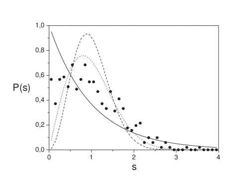
Figure 1: Distribution of level spacings –normalized to unit average– for the cnot baker map (big dots). The dimensions are 32 and 16 for the control and target bakers, respectively. We also display the predictions of random matrix theory (dotted line: GOE, dashed: GUE) and the Poisson distribution (full line).

The classical controlled-not baker ${\bf b}_{\textsc{cnot}}:(p_{0},q_{0})\rightarrow(p_{1},q_{1})$, corresponding to the unitary operator (21), is

$$p_{1}^{c} = \frac{1}{2}(p_{0}^{c}+\epsilon_{0}^{c})\;,$$ (26)

$$q_{1}^{c} = 2q_{0}^{c}-\epsilon_{0}^{c}\;,$$ (27)

$$p_{1}^{t} = \frac{1}{2}(p_{0}^{t}+\epsilon_{0}^{t}+\epsilon_{0}^{c}-2\epsilon_{0}^{t}\epsilon_{0}^{c})\;,$$ (28)

$$q_{1}^{t} = 2q_{0}^{t}-\epsilon_{0}^{t}\;.$$ (29)

Thus the classical orbits depend on the binary digits, $\epsilon_{0}^{c}$ and $\epsilon_{0}^{t}$ in an unsymmetric way. The orbit of the control subsystem is independent of the behaviour of the target, while the evolution of the principal binary digit of the control, that results from its internal chaotic motion, affects the target. This influence is as random as a perfect coin toss, so the control can be considered as a perfect Markovian environment for the target.

It is important to distinguish the classical trajectories of the full 4-dimensional map, from its projections into the 2-dimensional phase space rectangles that describe each of the subsystems. The full trajectory is deterministic, which is also the case for its projection onto the control phase space. It is the projection onto the target phase space that acquires an important random component, when knowledge of the control orbit is deleted. Viewed from the control phase space, we find an infinite number of trajectories of the full system that project onto the same control orbit.

Viewed within quantum mechanics, the relation between the subsystems becomes less unsymmetrical. Their entanglement is usually measured with reference to the reduced density matrix of either subsystem, that is ${\hat{\rho}}_{c}$, or ${\hat{\rho}}_{t}$, such as the purity, ${\rm tr}~{}{\hat{\rho}}^{2}$, or, equivalently, the linear entropy Nielsen ,

$$S_{L}=1-{\rm tr}~{}{\hat{\rho}}^{2}\;.$$ (30)

The effect of the entanglement is an increase of linear entropy from that of an initial product state, for which $S_{L}=0$. These measures are necessarily the same for both subsystems, no matter how lopsided the interaction Nielsen . Nonetheless, it is legitimate to consider the target subsystem of the controlled-not baker interaction as an ideal candidate for a quantum Markovian system. It is this picture of the control as forming an environment for the target that shall be studied below, rather than the alternative investigation of the entanglement of the principal qubits, with local environments taken as the set of remaining qubits of the controlled-not baker. The latter is the line taken in ScottCaves .

IV Evolution of entanglement: the Markovian limit

We considered the unitary evolution of the quantum controlled-not baker map, given initial product states, $|\psi\rangle_{c}\otimes|\psi\rangle_{t}$. Both of these factor states were chosen randomly with respect to the unitarily invariant Haar measure for pure states within both the control subsystem and the target subsystem Zanardi . Figure 2 show the evolution of the linear reduced entropy for either subsystem as a function of the discrete time, i.e. the number of iterations. In each of these figures the dimension of the target space was kept fixed at $D_{t}=16$, that is, four qubits. However, the size of the environmental control subspace grows from $D_{c}=4$ in (a) to $D_{c}=256$ in (d), i.e. eight qubits. In all cases the linear entropy rises sharply during the first five iterations, or so, and then oscillates around a stable average value, which depends on the choice of initial state. The asymptotic values for the entropy can be compared with those of random states ScottCaves . The average value of the linear reduced entropy for the Haar ensemble appropriate to the full Hilbert space is less than maximal ScottCaves ; Lubkin :

$$\langle S_{L}\rangle=1-\frac{D_{c}+D_{t}}{D_{c}D_{t}+1}\;.$$ (31)

In each of the above figures the Haar average is seen to lie within the fluctuations of the evolution of the individual states. This means that the entangling power Zanardi of the cnot baker is very close to that of a random operator Emerson . Another striking effect of increasing the dimension $D_{c}$ is the decrease in the amplitude of the fluctuations in linear entropy about their mean. This is in line with the decrease of the variance of the purity in the Haar ensemble as the dimension of the subsystems are increased ScottCaves .

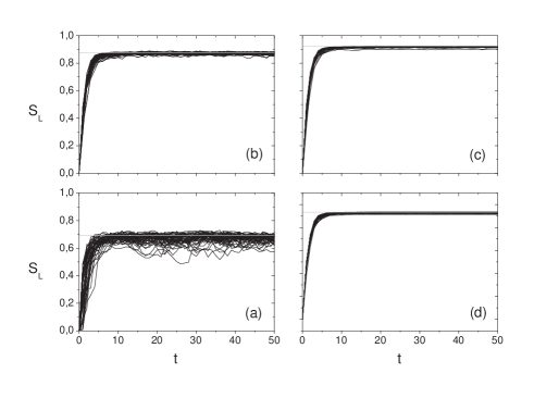
Figure 2: Linear entropy as a function of the number of iterations of the cnot baker. The dimension of the target space is fixed at $D_{t}=16$, but the size of the control subspace is increasing: $D_{c}$ = 4 (a), 16 (b), 64 (c), 256 (d). In each case we considered 50 initial product states chosen according to the (product) Haar measure. Also shown are the entropies of corresponding random states (horizontal lines).

Let us now compare this behaviour of the linear entropy of the target subsystem with that of the Markovian system:

$${\hat{\rho}}_{t}(1)={1\over 2}\left(\widehat{B}{\hat{\rho}}_{t}(0)\widehat{B}^{\dagger}+\widehat{B^{\prime}}{\hat{\rho}}_{t}(0)\widehat{B^{\prime}}^{\dagger}\right)\;.$$ (32)

That is, we average over the two possible stackings of the quantum baker map within the standard formalism of Kraus superoperators Breuer . This Markovian evolution is shown in Figure 3 for a set of random initial target states as in Fig. 2, so that for $D_{t}=16$. Evidently, the closest correspondence is verified with Fig. 2(d), which has the largest control space. Even though the target only interacts directly with the principal qubit of the control space, the internal motion within the latter is required to wash away information concerning the evolution of the target.

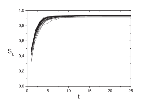
Figure 3: Markovian limit for the target map of the cnot baker. Shown is the linear entropy as a function of the number of iterations of the superoperator of Eq. (32). The dimension of the target space is $D_{t}=16$. We chose 50 initial product states according to the Haar measure.

Since the Markovian approximation presupposes complete randomness for the initial state of the environment, it is more appropriate to compare this irreversible evolution with the unitary evolution of a density operator defined as a product of a pure target state with a mixed control state. The latter is chosen to be proportional to the identity operator, i.e. it has equal weight for all basis state projectors in the control subsystem. Figure 4 displays the growth of the linear reduced entropy for a single initial state chosen randomly for various dimensions of the control subspace, $D_{c}$. This is strong evidence that the unitary evolution of the linear entropy converges onto the Markovian evolution in the limit where $D_{c}\rightarrow\infty$.

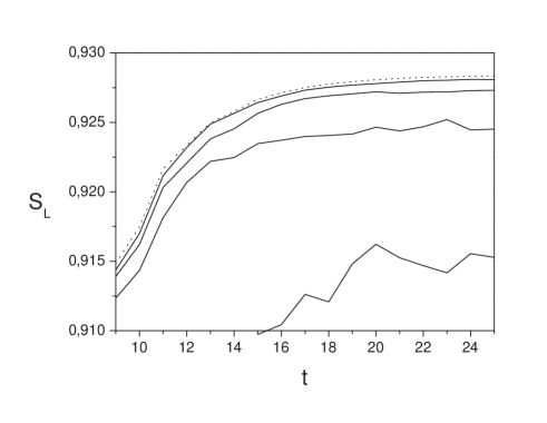
Figure 4: Comparison of Markovian vs. unitary evolution. (i) A single randomly-chosen initial state of the target system was evolved with the Markovian Eq. (32). (ii) The same target state, tensored with the identity of the environment, was evolved with the full unitary dynamics. In both cases we plot the linear entropies as a function of time. The Markovian case corresponds to the dotted line. Full lines represent the unitary evolution for environment sizes $D_{t}=8,16,32,64$. The dimension of the target space is fixed at $D_{t}=16$.

Most of the eigenvalues of the Markovian superoperator that acts on ${\hat{\rho}}_{t}(0)$ in (32) lie within the unit circle, as shown in Figure 5. In time, only the projection of the initial density operator with $\lambda=1$ remains. However, this eigenvalue is doubly degenerate, corresponding to both the identity operator and the reflection operator, defined by $\hat{R}|q_{m}\rangle=|1-q_{m}\rangle$ (the reflection is a symmetry of the individual baker maps Saraceno ). The fact that different initial density operators also differ in their projections onto this pair of states accounts for the spread in the asymptotic values of the respective linear entropies.

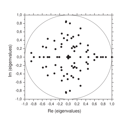
Figure 5: Eigenvalues of the Markov superoperator. The dimension of the target is $D_{t}=16$.

V Discussion

The general idea of a baker map is that “vertical” rectangular partitions of the unit square are stretched horizontally and squeezed vertically and then stacked. The generalization to partitions of $2L$-dimensional hypercubes is obvious, so that these then model a system with $L$ degrees of freedom. We have here shown that the different stacking orders allowed by higher dimensional baker maps may be interpreted as resulting from the various interactions of the principal qubits for each subsystem, if each of these is quantized to have a finite Hilbert space of dimension $D_{j}=2^{n_{j}}$. As a first exploration of such systems we have chosen the controlled-not baker map, where the interaction of the principal qubits is the universal cnot gate for quantum computation. We have discussed other possibilities for $L=2$ and there are many more for increasing $L$.

It is also possible to couple a baker map to some other simple unitary evolution. In the case of Ermann, Paz and Saraceno EPS , the latter corresponds to a pair of translations. Then the control map decides the direction of the displacement, rather than a stacking order for the target map. Such a quantum random walk does not belong to the class of generalized baker maps, because the target is not a chaotic system.

A further more elaborate possibility for interaction involves a rotation of the four parallelepipeds into which the primary digits of both maps divide a four dimensional phase space. Choosing this to be of $\pi/4$, shuffles the parallelepipeds, so that the doubled binary description is respected. This system is studied in Santoro . The interesting point is that the equilibrium and all the classical periodic orbits become “loxodromic”, i.e. the positions spiral outwards, while the momenta spiral inwards, because the eigenvalues of the stability matrix are general complex numbers. So far, not much effort has been made towards quantizing loxodromic motion, but Rivas is an exception.

Unlike the case of the various quantizations of a single baker proposed by Scott and Caves ScottCaves , there is a natural partition into the separate Hilbert spaces for interacting baker maps, with perfect classical correspondence. We can analyze the entropy evolution for the reduced density matrix of a single subsystem for each form of coupling. The other clear alternative is to trace out the density matrix of the secondary qubits for each component baker, so as to obtain a mixed state for each principal qubit. Then their entanglement is uniquely determined by the concurrence Wootters .

The remarkable facility for computing numerically the evolution of both quantum and classical baker maps extends to their higher dimensional couplings. Here we have provided numerical evidence that the generalized controlled-not baker map may be an ideal model for Markovian evolution of the target map, once the environmental control map is traced away. It is interesting to note that the interaction with the environment is not weak in any usual sense.

- (1) M. Saraceno and A. Voros, Physica D 79, 206 (1994).
- (2) R. Schack, Phys. Rev. A 57, 1634 (1998).
- (3) A. T. Brun and R. Schack, Phys. Rev. A 59, 2649 (1999)
- (4) Y. S. Weinstein, S. Lloyd, J. Emerson, and D. G. Cory, Phys. Rev. Lett. 89, 284102 (2002).
- (5) R. Schack and C. M. Caves, Appl. Algebra Eng. Commun. Comput. 10, 305 (2000).
- (6) N. L. Balazs and A. Voros, Ann. Phys. (NY) 190, 1 (1989).
- (7) M. Saraceno M 1990, Ann. Phys. (NY) 199, 37 (1990).
- (8) A. J. Scott and C. M. Caves, J. Phys. A 36, 9553 (2003).
- (9) See for example the review by O. Bohigas in M. J. Giannoni, A. Voros and J. Zinn-Justin (Eds.), Proc. Les Houches Summer School 1989, Chaos and Quantum Physics (North-Holland, Amsterdam, 1991).
- (10) A. Nielsen and I. Chuang, Quantum Computation and Quantum Information (Cambridge University Press, 2000).
- (11) M. C. de Oliveira and W. J. Munro Phys. Rev. A 61, 042309 (2000).
- (12) A. M. Ozorio de Almeida and M. Saraceno, Ann. Phys. (NY) 210, 1 (1991).
- (13) M. Sano, CHAOS 10, 195 (2000).
- (14) E. B. Bogomolny, B. Georgeot, M.-J. Giannoni and C. Schmit, Phys. Rep. 291, 219 (1997).
- (15) P. Zanardi, C. Zalka, and L. Faoro, Phys. Rev. A, 62, 030301 (2000).
- (16) E. Lubkin, J. Math. Phys. 19, 1028 (1978).
- (17) J. Emerson, Y. S. Weinstein, M. Saraceno, S. Lloyd, and D. G. Cory, Science 302, 2098 (2003).
- (18) H.-P. Breuer and F. Petruccione, Open Quantum Systems (Oxford University Press, 2002).
- (19) L. Ermann, J.P. Paz and M. Saraceno, quant-ph/0510037 (2005).
- (20) P. R. del Santoro, PhD Thesis (in preparation).
- (21) A. M. F. Rivas, M. Saraceno and A. M. Ozorio de Almeida Nonlinearity 13, 341 (2000).
- (22) W. K. Wootters, Phys. Rev. Lett. 80, 2245 (1998).