Exchange Energy in Coupled Quantum Dots

Abstract

In this work, the exchange energy $J$ for a system of two laterally-coupled quantum dots, each one with an electron, is calculated analytically and in a detailed form, considering them as hydrogen-like atoms, under the Heitler-London approach. The atomic orbitals, associated to each quantum dot, are obtained from translation relations, as functions of the Fock-Darwin states. Our results agree with the reported ones by Burkard, Loss and DiVincenzo in their model of quantum gates based on quantum dots, as well as with some recent experimental reports.

I Introduction

In the last decade, a great interest in quantum dotsjacak has arouse, due to their potential use as hardware for the implementation of a scalable quantum computerloss ; sherwin . In this scheme, the electron spin in these quantum dots is used as the basic element for the transport of information (qubit). Considering the fact that 1-$qubit$ and 2-$qubit$ gates are sufficient to make any quantum algorithm barenco ; divincenzo , a quantum computing device, based on quantum dots, must have a mechanism by which two specific qubits could be entangled to produce a fundamental 2-qubit quantum gate, such as the Controlled-NOT gate $XOR$loss . This process is achieved through single qubits rotations and an adequate switching of exchange energy $J(t)$ between the electronic spins $\mathbf{S_{1}}$ and $\mathbf{S_{2}}$ described by the Heisemberg spin exchange hamiltonian for a system of two laterally quantum dots, under the influence of a magnetic field, perpendicular to their surface. This is the reason for the studies of quantum gates with coupled quantum dots are reduced to get experimental control of the single qubits rotationscerletti and the exchange energy. In this work, considering the Heitler-Londonheitler approach, we present the process to obtain an expression of $J$ for this system as a function of parameters that allow its experimental control, with a detailed description which is not available in the work of Burkardburkard .

II Theory model of two laterally coupled quantum dots

Let us consider a system of two laterally coupled quantum dots, each one with an electron, constituted by electrical gating of two-dimensional electron gas (2DEG), under the action of a $z$-axis parallel magnetic field $\mathbf{B}$, and an electric field $\mathbf{E}$ in $x$-direction. Its physical representation is given by

$$H_{t}=H_{1}+H_{2}+V_{12}+W,$$ (1)

where $H_{j}$ is the Hamiltonian for the $1$ and $2$ quantum dot, and this is

$$H_{j}=\frac{1}{{2\mu}}\left[{\mathbf{p}_{j}+\frac{q_{e}}{c}\mathbf{A(r)}}\right]^{2}+eEx_{j}+\frac{\omega_{0}^{2}\mu}{2}\left[{(x_{j}\pm a)^{2}+y_{j}^{2}}\right],$$ (2)

The Coulomb interaction is given by $V_{12}$ , and $W=W_{1}+W_{2}$ represent a quartic potential for each quantum dot and it is written as

$$W_{i}=\frac{{\mu\omega_{0}^{2}}}{2}\left[{\frac{1}{{4a^{2}}}(x_{i}^{2}-a)^{2}-(x_{i}\pm a)^{2}}\right]^{2};\ \ \ \ i=1,2,$$ (3)

This potential models the effect of tunneling between the two quantum dots and its choice is motivated by experimental evidencetarucha ; kouwenhoven . Considering a low-temperature description, where the system is in a condition $kT<\hbar\omega_{0}$, we can only assume the two lower orbital states of the Hamiltonian $H_{t}$, which are singlet and triplet states. With these conditions, and without considering Zeeman effect and spin-orbit coupling, it is possible to translate this physical picture into the Heisenberg spin Hamiltonian, which is

$$H_{t}=J\ \mathbf{S_{1}}\cdot\mathbf{S_{2}}$$ (4)

This Hamiltonian is the scalar product between the spin operators and the factor $J$, which is the exchange energy between the spin triplet and singlet statesmattis .

III Wave Functions of Coupled Quantum Dots

In order to apply the Heitler-London approachheitler , it is primarily necessary to determine the wave function of each quantum dot, that constitutes our laterally coupled system, on which an $xy$-axis electric field and a $z$-axis magnetic field act.

Considering symmetric translation operations on a quantum system, through an scheme similar to the one used in the solution of a charged harmonic oscillator in a uniform electric fieldcohen , it is possible to get the eigenfunctions of (1) for $j=1,2$. To do this, we write (1) as a momentum translation $p_{jy}$ of the Fock-Darwin hamiltonian plus a constant depending of the electric field. The ground state of the Hamiltonians $H_{1}$ and $H_{2}$ are,

$$\phi_{0}^{(j)}=exp\left[-\Gamma{(j)}\right]\sqrt{\frac{m\Omega}{\pi\hbar}}\ exp\left[-\frac{m\Omega}{2\hbar}\left(x_{\mp}^{2}+y^{2}\right)\right],$$ (5)

for j=1,2, where

$$\Gamma_{(j)}=\frac{i}{\hbar}\left(\frac{q_{e}^{2}BE}{2m\omega_{0}^{2}c}\pm\frac{eBa}{2c}\right)y,$$ (6)

with $x_{\pm}=x\pm a+\frac{q_{e}E}{m\omega{0}}$, $q_{e}$ is the electron charge, $c$ is the light speed, $\mathbf{E}=(E,0,0)$, $\mathbf{B}=(0,0,B)$, $\Omega$ represents the Fock-Darwin frequency, $\omega_{0}$ the confinement frequency, and $\mathbf{A(r)}=\frac{\mathbf{B}}{2}(-y,x,0)$ the vector potential. These wave functions correspond to Fock-Darwin statesjacak translated a certain amount of momentum $p_{jy}=p_{jy}+\frac{q_{e}^{2}BE}{2m\omega_{0}^{2}c}\pm\frac{eBa}{2c}$.

IV The Heitler-London approach

A technique that allows to determine the exchange energy factor is to adapt the Heitler-London methodheitler (also known as valence orbit approximation) to our system, considering that it behaves as a pair of hydrogen-like artificial atoms. The symmetric (singlet) and antisymmetric (triplet) states are represented by

$$\left|\psi_{\pm}\right\rangle=\frac{\left|A(1)B(2)\right\rangle\pm\left|A(2)B(1)\right\rangle}{\sqrt{2(1\pm S^{2})}}.$$ (7)

Applying the Heitler-London method on our system, we have

$$\left.\begin{array}[]{l}A(j)=\phi_{0}^{(1)}(x_{j},y_{j})\\ B(j)=\phi_{0}^{(2)}(x_{j},y_{j})\\ \end{array}\right\}{\rm{}}j=1,2.$$ (8)

The parameter $S$ represents the overlapping between left and right orbital in each dot. This term is given by

$$S=\left\langle\phi_{0}^{(2)}|\phi_{0}^{(1)}\right\rangle,$$ (9)

with

$$b=\frac{\Omega}{{\omega_{0}}},\ \ \ \ d=a\sqrt{m\omega_{0}/\hbar},$$ (10)

where $a$ is half the distance between the centers of the dots, $a_{B}=\sqrt{\hbar/m\omega_{0}}$ is the effective Bohr radius of a single isolated harmonics well, $d$ is the dimensionless distance, and $b$ is a magnetic compression factor of the quantum dots orbitals.

V Exchange Energy

According to the magnetism theorymattis , the exchange energy is represented by

$$J=\epsilon_{t}-\epsilon_{s}=\left\langle{\psi_{-}}\right|H_{t}\left|{\psi_{-}}\right\rangle-\left\langle{\psi_{+}}\right|H_{t}\left|{\psi_{+}}\right\rangle,$$ (11)

where $\epsilon_{t}$ represents the triplet energy, $\epsilon_{s}$ singlet energy, and $H_{t}$ is described by (1). Introducing this term in (11), and regrouping common terms we obtain

$$J=\frac{S^{2}}{1+S^{4}}\bigl{[}\Upsilon_{1}-\frac{\Upsilon_{2}}{S^{2}}+\Upsilon_{3}-\frac{\Upsilon_{4}}{S^{2}}+\Upsilon_{5}\bigr{]},$$ (12)

where

$$\Upsilon_{1}=\left\langle A(1)\right|H_{1}\left|A(1)\right\rangle\left\langle B(2)|B(2)\right\rangle\\ +\left\langle B(2)\right|H_{2}\left|B(2)\right\rangle\left\langle A(1)|A(1)\right\rangle\\ +\left\langle B(1)\right|H_{1}\left|B(1)\right\rangle\left\langle A(2)|A(2)\right\rangle\\ \left\langle A(2)\right|H_{2}\left|A(2)\right\rangle\left\langle B(1)|B(1)\right\rangle,$$ (13)

$$\Upsilon_{2}=\left\langle A(1)\right|H_{1}\left|B(1)\right\rangle\left\langle B(2)|A(2)\right\rangle\\ +\left\langle B(2)\right|H_{2}\left|A(2)\right\rangle\left\langle A(1)|B(1)\right\rangle\\ +\left\langle B(1)\right|H_{1}\left|A(1)\right\rangle\left\langle A(2)|B(2)\right\rangle\\ \left\langle A(2)\right|H_{2}\left|B(2)\right\rangle\left\langle B(1)|A(1)\right\rangle,$$ (14)

$$\Upsilon_{3}=\left\langle A(1)B{(2)}\right|V_{12}\left|A(1)B{(2)}\right\rangle\\ +\left\langle A(2)B{(1)}\right|V_{12}\left|A(2)B{(1)}\right\rangle,$$ (15)

$$\Upsilon_{4}=\left\langle A(1)B{(2)}\right|V_{12}\left|A(2)B{(1)}\right\rangle\\ +\left\langle A(2)B{(1)}\right|V_{12}\left|A(1)B{(2)}\right\rangle,$$ (16)

$$\Upsilon_{5}=\left\langle A(1)B{(2)}\right|W_{1}+W_{2}\left|A(1)B{(2)}\right\rangle\\ +\left\langle A(2)B{(1)}\right|W_{1}+W_{2}\left|A(2)B{(1)}\right\rangle\\ -\frac{1}{S^{2}}\bigl{[}\left\langle A(2)B{(1)}\right|W_{1}+W_{2}\left|A(1)B{(2)}\right\rangle\\ +\left\langle A(1)B{(2)}\right|W_{1}+W_{2}\left|A(2)B{(1)}\right\rangle\bigr{]}.$$ (17)

The solution of the term $\Upsilon_{1}$ (13) does not have higher difficult if we take that $\left\langle A(j)|A(j)\right\rangle=\left\langle B(j)|B(j)\right\rangle=1$. For the next term $\Upsilon_{2}$ (14) it is easily to demonstrate that $\left\langle A(j)|B(j)\right\rangle=\left\langle B(j)|A(j)\right\rangle=S$. The solutions of $\Upsilon_{3}$ (15) and $\Upsilon_{4}$ (16) are obtained using the center of mass and relative coordinates. The next step is to make a change from cartesian coordinates to polar coordinates. In this process, four kind of quadratures of many special functions appear, which are resolved making use of the expansions given in abramowitz and gradshteyn . In order to determine $\Upsilon_{5}$ (17) we write $\left\langle A(2)B{(1)}\right|W_{1}+W_{2}\left|A(2)B{(1)}\right\rangle$ in terms of $\left\langle A(1)B{(2)}\right|W_{1}+W_{2}\left|A(1)B{(2)}\right\rangle$ and the rest of terms are calculated considering translation operations in $p_{y}$ and $x$. Finally, replacing (9), and the solutions of (13) - (17) in (12) we find

$$J(B,E,d)=\frac{\hbar\omega_{0}}{\sinh\bigl{(}2d^{2}\bigl{[}2b-\frac{1}{b}\bigr{]}\bigr{)}}\Biggl{[}c\sqrt{b}\Biggr{(}e^{-bd^{2}}\mathbf{I}_{0}\left(bd^{2}\right)\\ -e^{d^{2}\left(b-1/b\right)}\mathbf{I}_{0}\left(d^{2}\left[b-1/b\right]\right)\Biggr{)}+\frac{3}{4b}\left(1+bd^{2}\right)\\ +\frac{3}{2}\frac{1}{d^{2}}\left(\frac{eEa}{\hbar\omega_{0}}\right)^{2}\Biggr{]}.$$ (18)

This is the exchange energy, and as we can notice, it presents dependence of external parameters such as $\mathbf{B}$, $\mathbf{E}$ and $d$.

VI Results

Eq. (18) describes the exchange energy $J$ and is constituted by four terms. The first and second terms are result of $\Upsilon_{3}$ and $\Upsilon_{4}$, in which the Coulomb interaction $V_{12}$ acts. The third term, in spite of having a polynomial behavior, avoids an abrupt decline that the two first terms offer. Since there is a difference of sign between the first and second term of Eq. (18), there exists a value of $\mathbf{B}=\mathbf{B^{*}}$ for which $J$ switches from positive to negative.

Figure 1: Exchange energy $J(B)$ in $meV$ plotted against the magnetic field for different electric fields, for $a=0.7a_{b}$ and $c=2.36.$ The most remarkable feature of $J$ is the change of its sign from positive to negative.

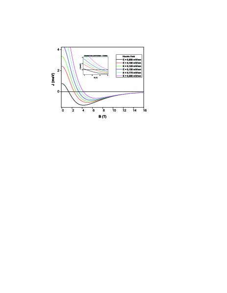
In Fig.1 we present the transition from antiferromagnetic $(J>0)$ to ferromagnetic $(J<0)$ spin-spin coupling, that occurs with the increasing of the magnetic field and is caused by long-range Coulomb interaction, in particular by the second term in Eq. (18) . For $\mathbf{B}>\mathbf{B^{*}}$, a compression of the orbitals appears, which reduces the overlap of the wavefunctions exponentially. In addition, in Fig.1 it is shown the behavior of $J(B)$ for some values of $E$. The fourth term in Eq. (18) reveals the dependence of $J$ with $E$. The increasing of the electric field produces a raise on the exchange energy. The increment of $E$ creates a displacement of the value $\mathbf{B^{*}}$, in which the sign switch of $J$ takes place. Thus, the most efficiency to tune the exchange energy $J$ is acquired for $E=0$.

Figure 2: Transition of exchange energy for $J(E)$. Instead of $J(B)$ and $J(d)$, the transition in this case is from ferromagnetic to antiferromagnetic.

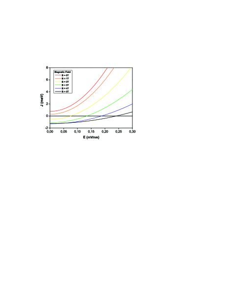
Fig.2. shows the behavior of $J(E)$, for $B$ and $d$ fixed. Here, it is observed that it is possible to produce a sign switch, but the transition is now from ferromagnetic $(J<0)$ to antiferromagnetic $(J>0)$ and only with an acting $B\geq 1.35$T field over the system. 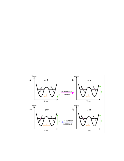This feature yields to think in a two quantum dots scheme, operating as a quantum gate, it could return to its initial state without eliminating the magnetic field interaction after the $J$ switching. If we consider that the transition is initially from antiferromagnetic to ferromagnetic, varying $B$ and fixing $E$ (Fig.3A-B), to return to its initial state we keep $B$ constant and increase $E$ until the system presents a transition from ferromagnetic to antiferromagnetic (Fig.3C-D).

Figure 3: Switching system for two laterally coupled quantum dots operating as a quantum gate.

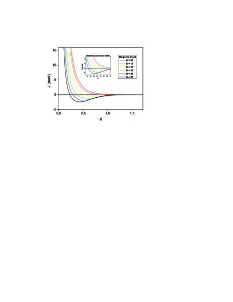
The behavior of the exchange energy as a function of $d$ is showed in Fig. 4. In this representation, for diverse values of $B$, and with $E=0$, if we vary $d$ between 0 and 1.5 a transition antiferro - ferro of $J$ is evident for $B>1T$. Similarly to Fig. 1, for $d>1$, the overlapping between the wave functions decreases exponentially. Another important characteristic which uncover the efficiency of this model is exhibited when an increase of the $B$ field is made, producing a diminution of the separation distance between the dots at which $J$ changes its sign.

Figure 4: Behavior of the exchange energy $J(d)$ as a function of the quantum dots separation, keeping the electric field constant, $E=0V$. We observe that the increasing of the magnetic field produces a diminution of the separation distance between the dots at which $J$ changes its sign.

In the last years, experiments of inelastic cotunneling for two electrons in a single gated quantum dots have led to carry out measurements of the exchange energy $J$zumbuhl , showing a high concordance with the already described in the theoretical model.

VII Conclusions

We achieve a detailed description of a satisfactory model which let us calculate the exchange energy factor $J$ analytically, for a system of two laterally coupled quantum dots, applying the Heitler-London formalism.
The calculation of $J$ as a function of parameters such as $E$, $B$ and $d$, and an adequate variation of them allows us to describe a control scheme in the sign of the exchange energy, which will help to produce qubits entanglement in the arquitecture of Loss and DiVincenzo.
Using a constant magnetic field over the two quantum dots it is possible to switch the exchange energy sign, by means of a changeable electric field, whose increase allows an antiferromagnetic to ferromagnetic transition.
A switching scheme of $J$ is also presented, which allows to a quantum gate reaching its initial state after computing certain operation, without eliminating the interactions of the electric and magnetic fields on the system.

Acknowledgments

H.E.Caicedo-Ortiz thank to A.I. Figueroa for technical support in the writing of this manuscript. S.T. Perez-Merchancano acknowledge financial support from the Vicerrectoria de Investigaciones - Universidad del Cauca for his displacement to the ”XII Latin American Congress of Surface Science and its applications CLACSA 2005”.

References

- (1) L. Jacak, P. Hawrylak and A. Wojs, Quantum Dots, Springer-Verlag Berlin Heidelberg, 1998.
- (2) D. Loss and D.P. DiVincenzo, Phys. Rev. A 57, 120 (1998).
- (3) M.S. Sherwin, A. Imamoglu and T. Montroy, Phys. Rev. A 60, 3508 (1999).
- (4) A. Barenco, C. Bennet, R. Clave, D. Divincenzo, N. Margolus, P. Shor, T Sleater, J. Smolin and H. Weinfurter, Phys. Rev A 52, 3457 (1995).
- (5) D.P. DiVincenzo, Phys. Rev A 51, 1015 (1995).
- (6) V. Cerletti., W.A. Coish, Oliver Gywat and D. Loss, Nanotechnology 16, R27 (2005).
- (7) W. Heitler and F. London, Z. physik 44, 455 (1927).
- (8) G. Burkard, D. Loss and D.P. DiVincenzo, Phys. Rev. B 59, 2070 (1999).
- (9) S. Tarucha, D.G. Austing, T. Honda, R. J. van der Hage and L.P. Kouwenhoven, Phys. Rev Lett. 77, 3613 (1996).
- (10) L. P. Kouwenhoven, T.H. Oosterkamp, M. W. S. Danoesastro, M. Eto, D.G. Austing, T. Honda and S. Tarucha, Science 278, 1788 (1997)
- (11) D. Mattis, The Theory of Magnetism, Harper & Row, 1965.
- (12) C. Cohen-Tannoudji, Quantum Mechanics Vol 1, Hermann and John Wiley & Sons, 1977.
- (13) M. Abramowitz and I.A. Stegun, Handbook of Mathematical Functions with Formulas, Graphs, and Mathematical Tables, Dover, 1964.
- (14) I.S. Gradshteyn and I.M. Ryzhik, Table of Integrals, Academic Press New York, 1994.
- (15) D. Zumbühl, C.M. Marcus, M.P. Handson and A.C. Grossard, Phys. Rev Lett. 93, 256801 (2004)