The rigged Hilbert space approach to the Lippmann-Schwinger equation. Part II: The analytic continuation of the Lippmann-Schwinger bras and kets

Abstract

The analytic continuation of the Lippmann-Schwinger bras and kets is obtained and characterized. It is shown that the natural mathematical setting for the analytic continuation of the solutions of the Lippmann-Schwinger equation is the rigged Hilbert space rather than just the Hilbert space. It is also argued that this analytic continuation entails the imposition of a time asymmetric boundary condition upon the group time evolution, resulting into a semigroup time evolution. Physically, the semigroup time evolution is simply a (retarded or advanced) propagator.

1 Introduction

This paper is devoted to construct and characterize the analytic continuation of the Lippmann-Schwinger bras and kets, as well as the analytic continuation of the “in” and “out” wave functions. This paper follows up on Ref. [1], where we obtained and characterized the solutions of the Lippmann-Schwinger equation associated with the energies of the physical spectrum. We showed in [1] that such solutions are accommodated by the rigged Hilbert space rather than by the Hilbert space alone. In this paper, we shall show that the analytic continuation of the Lippmann-Schwinger bras and kets is also accommodated by the rigged Hilbert space rather than by the Hilbert space alone.

It was shown in Ref. [1] that the Lippmann-Schwinger bras and kets are distributions that act on a space of test functions $\mathbf{\Phi}\equiv{\cal S}(\mathbb{R}^{+}\!\frac{\ }{\ }\{a,b\})$. The space $\mathbf{\Phi}$ arises from invariance under the action of the Hamiltonian and from the need to tame purely imaginary exponentials. These two requirements force the functions of $\mathbf{\Phi}$ to have a polynomial falloff at infinity. The resulting $\mathbf{\Phi}$ is a space of test functions of the Schwartz type. In this paper, it is shown that the analytic continuation of the Lippmann-Schwinger bras and kets are distributions that act on a space of test functions ${\mathbf{\Phi}}_{\rm exp}$. The space ${\mathbf{\Phi}}_{\rm exp}$ arises from invariance under the action of the Hamiltonian and from the need to tame real exponentials. These two requirements force the elements of ${\mathbf{\Phi}}_{\rm exp}$ to fall off at infinity faster than real exponentials. More precisely, we shall ask the elements of ${\mathbf{\Phi}}_{\rm exp}$ to fall off faster than Gaussians. The resulting ${\mathbf{\Phi}}_{\rm exp}$ is therefore of the ultra-distribution type. We recall that an ultra-distribution is an infinitely differentiable test function that falls off at infinity faster than exponentials.

In Ref. [1], we obtained the time evolution of wave functions and of the Lippmann-Schwinger bras and kets associated with real energies, and we saw that it is given by the standard quantum mechanical group time evolution. In this paper, we shall see that analytically continuing the time evolution of the wave functions results into a semigroup. We shall argue, although not fully prove, that analytically continuing the time evolution of Lippmann-Schwinger bras and kets also results into a semigroup.

As in Ref. [1], we restrict ourselves to the spherical shell potential

$$V({\bf x})\equiv V(r)=\left\{\begin{array}[]{ll}0&0<r<a\\ V_{0}&a<r<b\\ 0&b<r<\infty\end{array}\right.$$ (1.1)

for zero angular momentum. Nevertheless, our results are valid for a larger class of potentials that include, in particular, potentials of finite range. The reason why our results are valid for such a large class of potentials is that, ultimately, such results depend on whether one can analytically continue the Jost and scattering functions into the whole complex plane. Since such continuation is possible for potentials that fall off at infinity faster than any exponential [2], our results remain valid for a whole lot of interesting potentials.

In this paper, there will be a change in notation with respect to Ref. [1]. In Ref. [1], we used the symbol $\psi^{-}$ to denote the “out” states, and $\varphi^{\rm in}$, $\psi^{\rm out}$ to denote the asymptotically free “in” and “out” states. In the present paper, for the sake of brevity, we shall use the symbol $\varphi^{-}$ to denote the “out” wave functions $\psi^{-}$, and $\varphi$ to denote any asymptotically free wave function such as $\varphi^{\rm in}$ or $\psi^{\rm out}$.

Throughout the paper, we shall always use radial analytic continuation, because the transformation $z\to\sqrt{z}$ converts a radial path of integration into another radial path, while it distorts horizontal paths of integration.

Since the physical spectrum of the spherical shell potential is $[0,\infty)$, one may wonder if performing analytic continuations is somehow inconsistent. To qualm any doubts, we recall that the $S$ matrix, which is defined and unitary on the physical spectrum, is routinely continued into the complex plane. Much the same way, one can continue the wave functions and the Lippmann-Schwinger bras and kets into complex energies.

An important point is what happens with the self-adjointness of the Hamiltonian on the space of test functions ${\mathbf{\Phi}}_{\rm exp}$ (and also on $\mathbf{\Phi}$). These spaces satisfy

$${\mathbf{\Phi}}_{\rm exp}\subset{\mathbf{\Phi}}\subset{\cal D}(H)\,,$$ (1.2)

where ${\cal D}(H)$ is the domain on which the Hamiltonian is self-adjoint [1]. Thus, on $\mathbf{\Phi}$ and ${\mathbf{\Phi}}_{\rm exp}$, the Hamiltonian is not a self-adjoint operator but just the restriction of a self-adjoint one.

As shall be shown, the analytically continued Lippmann-Schwinger bras and kets are eigenvectors of the Hamiltonian with complex eigenvalues, and one may naturally wonder whether such complex eigenvalues are in conflict with the self-adjointness of the Hamiltonian, which in principle forbids any complex eigenvalues. To see how self-adjoint operators can have complex eigenvalues, let us consider the 1D momentum operator $P=-\rmi\hbar\rmd/\rmd x$. The eigenfunctions of $P$ are $\rme^{\rmi px/\hbar}$ with eigenvalue $p$. The eigenvalue $p$ can in principle be any complex number, although of course the physical spectrum of $P$ is the real line and in the completeness relation there only appear real $p$. Similarly, the eigenvalue equation for the spherical shell Hamiltonian is valid for any complex number (if additional boundary conditions are not imposed). Needless to say, the eigenfunctions of the Hamiltonian with complex eigenvalues are not in the Hilbert space –they are distributions– and thus there arises no conflict with the self-adjointness of the Hamiltonian.

Analytic continuations of the Lippmann-Schwinger equation have also been performed in [3, 4, 5, 6, 7, 8, 9] by assuming that, in the energy representation, the Lippmann-Schwinger bras and kets act on two different spaces of Hardy functions. Contrary to [3, 4, 5, 6, 7, 8, 9], we shall not make any a priori assumption. Rather, we shall simply obtain the analytic continuation and study its properties. As it turns out, the analytically continued Lippmann-Schwinger bras and kets do not act on spaces of Hardy functions. Therefore, our results differ drastically from those of [3, 4, 5, 6, 7, 8, 9].

The rigged Hilbert space we shall use is very similar to, although not the same as the rigged Hilbert space used by Bollini et al. to describe the resonance (Gamow) states [10, 11]. There are two major differences. First, Bollini et al. use a space of test functions that fall off at infinity faster than exponentials, whereas we shall use test functions that fall off faster than Gaussians. The advantage of using Gaussian falloff is that, as will be discussed elsewhere, one can obtain meaningful resonance expansions. Second, Bollini et al. obtain many results by using the momentum representation and the Fourier transform, whereas the present paper deals with the wave-number representation and the Fourier-like transforms ${\cal F}_{\pm}$ of Sec. 2. The advantage of the wave-number representation is that in such representation, the Hamiltonian acts as a multiplication operator, whereas in the momentum representation, the Hamiltonian acts as a complicated integral operator. The simplicity of the wave-number representation will allow us to go beyond the results of [10, 11].

The ultimate goal we want to achieve by analytically continuing the solutions of the Lippmann-Schwinger equation is to obtain the resonance states. Although this point will be treated elsewhere, we want to present a brief preview of the results. The resonance states are usually obtained by solving the Schrödigner equation subject to purely outgoing boundary conditions, but they can also be obtained by analytically continuing the Lippmann-Schwinger bras and kets into the resonance energies. The results of this paper will enable us to do just so, and to obtain some novel properties of the Gamow states. The resulting Gamow states will turn out to be different from the so-called “Gamow vectors” of [4].

The structure of the paper is as follows. In Sec. 2, we rewrite the results of Ref. [1] in terms of the wave number, because the analytic continuation is more easily done in terms of the wave number than in terms of the energy.

In Sec. 3, we analytically continue the Lippmann-Schwinger and the “free” eigenfunctions. As well, we characterize the analytic and the growth properties of such continued eigenfunctions.

In Sec. 4, we make use of the eigenfunctions of Sec. 3 to analytically continue the Lippmann-Schwinger and the “free” bras and kets.

In Sec. 5, we construct the rigged Hilbert spaces that accommodate the analytically continued bras and kets of Sec. 4, and we use these rigged Hilbert spaces to show that the analytically continued bras and kets are eigenvectors of the Hamiltonian.

In Sec. 6, we construct and characterize the wave number representation of the rigged Hilbert spaces, bras, kets and wave functions. In particular, we characterize the analytic and growth properties of the analytically continued wave functions in the wave number representation. By means of Gelfand’s and Shilov’s $M$ and $\Omega$ functions [12], we shall see how the exponential falloff of the elements of ${\mathbf{\Phi}}_{\rm exp}$ in the position representation limits the growth of those elements in the wave number representation.

In Sec. 7, we construct the time evolution of the analytically continued wave functions, bras and kets. By using the results of Sec. 6, we shall see that the analytic continuation of the group time evolution of the wave functions entails the imposition of a time asymmetry that converts the group time evolution into a semigroup. Such semigroup is just a (retarded or advanced) propagator. We shall also argue, although not fully prove, that the time evolution of the analytically continued Lippmann-Schwinger bras and kets is also given by semigroups.

In Sec. 8, we discuss the relation between time asymmetry and the $\pm\rmi\varepsilon$ of the Lippmann-Schwinger equation. Finally, in Sec. 9, we state our conclusions.

All through this paper, $C$ will denote positive constants, not necessarily the same at each appearance.

2 The wave number representation

The eigenfunctions of the time independent Schrödinger equation depend explicitly not on the energy $E$ but on the wave number $k$ [1],

$$k=\sqrt{\frac{2m}{\hbar^{2}}E\,}\,.$$ (2.1)

In particular, the Lippmann-Schwinger eigenfunctions and the eigenfunction expansions depend explicitly on $k$ rather than on $E$. It is therefore convenient to rewrite their expressions in terms of $k$ before performing analytic continuations.

2.1 The Lippmann-Schwinger eigenfunctions in terms of the (positive) wave number

We start by writing the regular solution in terms of $k$:

$$\chi(r;k)=\chi(r;E)=\left\{\begin{array}[]{lll}\sin(kr)&0<r<a\\ {\cal J}_{1}(k)\rme^{\rmi\kappa r}+{\cal J}_{2}(k)\rme^{-\rmi\kappa r}&a<r<b\\ {\cal J}_{3}(k)\rme^{\rmi kr}+{\cal J}_{4}(k)\rme^{-\rmi kr}&b<r<\infty\,,\end{array}\right.$$ (2.2)

where

$$\kappa=\sqrt{\frac{2m}{\hbar^{2}}(E-V_{0})\,}=\sqrt{k^{2}-\frac{2m}{\hbar^{2}}V_{0}\,}\ .$$ (2.3)

In terms of $k$, the Lippmann-Schwinger eigenfunctions read as

$$\chi^{\pm}(r;E)=\sqrt{\frac{1}{\pi}\frac{2m/\hbar^{2}}{k}\,}\,\frac{\chi(r;k)}{{\cal J}_{\pm}(k)}\,.$$ (2.4)

The eigenfunctions $\chi^{\pm}(r;E)$ are $\delta$-normalized as functions of $E$:

$$\int_{0}^{\infty}\rmd r\,\overline{\chi^{\pm}(r;E)}\chi^{\pm}(r;E^{\prime})=\delta(E-E^{\prime})\,.$$ (2.5)

The Lippmann-Schwinger eigenfunctions that are $\delta$-normalized as functions of $k$ are given by

$$\chi^{\pm}(r;k):=\sqrt{\frac{\hbar^{2}}{2m}2k\,}\,\chi^{\pm}(r;E)=\sqrt{\frac{2}{\pi}\,}\,\frac{\chi(r;k)}{{\cal J}_{\pm}(k)}\,.$$ (2.6)

Indeed, it is easy to check that

$$\int_{0}^{\infty}\rmd r\,\overline{\chi^{\pm}(r;k)}\chi^{\pm}(r;k^{\prime})=\delta(k-k^{\prime})\,.$$ (2.7)

2.2 The “in” and “out” bras, kets and wave functions in terms of the (positive) wave number

Once we have expressed the Lippmann-Schwinger eigenfunctions as $\delta$-normalized eigenfunctions of $k$, we can construct the unitary operators that transform from the position into the wave number representation. These operators will be denoted by ${\cal F}_{\pm}$. We shall also rewrite the Lippmann-Schwinger bras and kets, along with the basis expansions induced by them, in terms of $k$.

We first define the wave number representation, $\widehat{f}(k)$, of any function $\widehat{f}(E)$ in $L^{2}([0,\infty),\rmd E)$ by

$$\widehat{f}(k):=\sqrt{\frac{\hbar^{2}}{2m}\,2k\,}\,\widehat{f}(E)\,.$$ (2.8)

Because $\widehat{f}(E)$ belongs to $L^{2}([0,\infty),\rmd E)$, the function $\widehat{f}(k)$ belongs to $L^{2}([0,\infty),\rmd k)$. The expressions for ${\cal F}_{\pm}$ and ${\cal F}_{\pm}^{-1}$ as integral operators can be easily obtained from the expressions for the operators $U_{\pm}$ and $U_{\pm}^{-1}$ of Ref. [1] with help from Eqs. (2.1), (2.6) and (2.8):

$$\widehat{f}_{\pm}(k)=({\cal F}_{\pm}f)(k)=\int_{0}^{\infty}\rmd r\,f(r)\overline{\chi^{\pm}(r;k)}\,,$$ (2.9a)

$$f(r)=({\cal F}_{\pm}^{-1}\widehat{f}_{\pm})(r)=\int_{0}^{\infty}\rmd k\,\widehat{f}_{\pm}(k)\chi^{\pm}(r;k)\,.$$ (2.9b)

By construction, ${\cal F}_{\pm}$ are unitary operators from $L^{2}([0,\infty),\rmd r)$ onto $L^{2}([0,\infty),\rmd k)$:

$$\begin{array}[]{rcl}{\cal F}_{\pm}:L^{2}([0,\infty),\rmd r)&\longmapsto&L^{2}([0,\infty),\rmd k)\\ f(r)&\longmapsto&\widehat{f}_{\pm}(k)=({\cal F}_{\pm}f)(k)\,.\end{array}$$ (2.9j)

The notation ${\cal F}_{\pm}$ intends to stress that ${\cal F}_{\pm}$ are Fourier-like transforms.

In terms of $k$, the Lippmann-Schwinger bras and kets become

$$\langle^{\pm}k|=\sqrt{\frac{\hbar^{2}}{2m}\,2k\,}\,\langle^{\pm}E|\,,\quad k>0\,,$$ (2.9ka)

$$|k^{\pm}\rangle=\sqrt{\frac{\hbar^{2}}{2m}\,2k\,}\,|E^{\pm}\rangle\,,\quad k>0\,;$$ (2.9kb)

that is,

$$\langle^{\pm}k|\varphi^{\pm}\rangle=\int_{0}^{\infty}\rmd r\,\langle^{\pm}k|r\rangle\langle r|\varphi^{\pm}\rangle\,,\quad k>0\,,\ \varphi^{\pm}\in{\mathbf{\Phi}}\,,$$ (2.9kla)

$$\langle\varphi^{\pm}|k^{\pm}\rangle=\int_{0}^{\infty}\rmd r\,\langle\varphi^{\pm}|r\rangle\langle r|k^{\pm}\rangle\,,\quad k>0\,,\ \varphi^{\pm}\in{\mathbf{\Phi}}\,,$$ (2.9klb)

where ${\mathbf{\Phi}}\equiv{\cal S}(\mathbb{R}^{+}\!\frac{\ }{\ }\{a,b\})$ is the Schwartz-like space built in [1] and

$$\langle r|k^{\pm}\rangle=\chi^{\pm}(r;k)\,,\quad k>0\,,$$ (2.9klma)

$$\langle^{\pm}k|r\rangle=\overline{\chi^{\pm}(r;k)}=\chi^{\mp}(r;k)\,,\quad k>0\,.$$ (2.9klmb)

Using the corresponding formal identity for the bras and kets in terms of $E$, one can express the identity operator as

$$1=\int_{0}^{\infty}\rmd k\,|k^{\pm}\rangle\langle^{\pm}k|\,;$$ (2.9klmn)

that is,

$$\langle r|\varphi^{\pm}\rangle=\int_{0}^{\infty}\rmd k\,\langle r|k^{\pm}\rangle\langle^{\pm}k|\varphi^{\pm}\rangle\,,\quad k>0\,,\ \varphi^{\pm}\in{\mathbf{\Phi}}\,.$$ (2.9klmo)

One can also express the $S$-matrix element as

$$(\varphi^{-},\varphi^{+})=\int_{0}^{\infty}\rmd k\,\langle\varphi^{-}|k^{-}\rangle S(k)\langle^{+}k|\varphi^{+}\rangle\,,\quad\varphi^{\pm}\in{\mathbf{\Phi}}\,,$$ (2.9klmp)

where

$$S(k)=\frac{{\cal J}_{-}(k)}{{\cal J}_{+}(k)}\,.$$ (2.9klmq)

Since in the energy representation $H$ acts as multiplication by $E$, in the wave number representation $H$ acts as multiplication by $\frac{\hbar^{2}}{2m}k^{2}$:

$$(\widehat{H}\widehat{f})(k)=({\cal F}_{\pm}H{\cal F}_{\pm}^{\dagger}\widehat{f})(k)=\frac{\hbar^{2}}{2m}k^{2}\,\widehat{f}(k)\,.$$ (2.9klmr)

As well, the bras $\langle^{\pm}k|$ and kets $|k^{\pm}\rangle$ are, respectively, left and right eigenvectors of $H$ with eigenvalue $\frac{\hbar^{2}}{2m}k^{2}$:

$$\langle^{\pm}k|H=\frac{\hbar^{2}}{2m}k^{2}\langle^{\pm}k|\,,$$ (2.9klms)

$$H|k^{\pm}\rangle=\frac{\hbar^{2}}{2m}k^{2}|k^{\pm}\rangle\,.$$ (2.9klmt)

2.3 The “free” bras, kets and wave functions in terms of the (positive) wave number

The expressions for the eigenfunctions, bras and kets of the free Hamiltonian $H_{0}$ can also be rewritten in terms of $k$.

The “free” eigenfunction that is $\delta$-normalized as a function of $k$ is given by

$$\chi_{0}(r;k):=\sqrt{\frac{\hbar^{2}}{2m}2k\,}\,\chi_{0}(r;E)=\sqrt{\frac{2}{\pi}\,}\,\sin(kr)\,.$$ (2.9klmu)

By using Eqs. (2.1), (2.8) and (2.9klmu), together with the expression for the integral operator $U_{0}$ obtained in Ref. [13], one can construct the following integral operator and its inverse:

$$\widehat{f}_{0}(k)=({\cal F}_{0}f)(k)=\int_{0}^{\infty}\rmd r\,f(r)\overline{\chi_{0}(r;k)}\,,$$ (2.9klmva)

$$f(r)=({\cal F}_{0}^{-1}\widehat{f}_{0})(r)=\int_{0}^{\infty}\rmd k\,\widehat{f}_{0}(k)\chi_{0}(r;k)\,.$$ (2.9klmvb)

The transform ${\cal F}_{0}$ is a unitary operator from $L^{2}([0,\infty),\rmd r)$ onto $L^{2}([0,\infty),\rmd k)$:

$$\begin{array}[]{rcl}{\cal F}_{0}:L^{2}([0,\infty),\rmd r)&\longmapsto&L^{2}([0,\infty),\rmd k)\\ f(r)&\longmapsto&\widehat{f}_{0}(k)=({\cal F}_{0}f)(k)\,.\end{array}$$ (2.9klmvw)

In terms of $k$, the “free” bras and kets become

$$\langle k|=\sqrt{\frac{\hbar^{2}}{2m}\,2k\,}\,\langle E|\,,\quad k>0\,,$$ (2.9klmvxa)

$$|k\rangle=\sqrt{\frac{\hbar^{2}}{2m}\,2k\,}\,|E\rangle\,,\quad k>0\,;$$ (2.9klmvxb)

that is,

$$\langle k|\varphi\rangle=\int_{0}^{\infty}\rmd r\,\langle k|r\rangle\langle r|\varphi\rangle\,,\quad k>0\,,$$ (2.9klmvxya)

$$\langle\varphi|k\rangle=\int_{0}^{\infty}\rmd r\,\langle\varphi|r\rangle\langle r|k\rangle\,,\quad k>0\,,$$ (2.9klmvxyb)

where

$$\langle k|r\rangle=\overline{\chi_{0}(r;k)}=\chi_{0}(r;k)\,,\quad k>0\,,$$ (2.9klmvxyza)

$$\langle r|k\rangle=\chi_{0}(r;k)\,,\quad k>0\,,$$ (2.9klmvxyzb)

and where $\varphi$ denotes either $\varphi^{\rm in}$ or $\psi^{\rm out}$.

Using the corresponding formal identity for the “free” bras and kets in terms of $E$, one can express the identity operator as

$$1=\int_{0}^{\infty}\rmd k\,|k\rangle\langle k|\,;$$ (2.9klmvxyzaa)

that is,

$$\langle r|\varphi\rangle=\int_{0}^{\infty}\rmd k\,\langle r|k\rangle\langle k|\varphi\rangle\,,\quad k>0\,.$$ (2.9klmvxyzab)

In the wave number representation $H_{0}$ acts as multiplication by $\frac{\hbar^{2}}{2m}k^{2}$:

$$(\widehat{H}_{0}\widehat{f})(k)=({\cal F}_{0}H_{0}{\cal F}_{0}^{\dagger}\widehat{f}_{0})(k)=\frac{\hbar^{2}}{2m}k^{2}\,\widehat{f}_{0}(k)\,.$$ (2.9klmvxyzac)

As well, the bras $\langle k|$ and kets $|k\rangle$ are, respectively, left and right eigenvectors of $H_{0}$ with eigenvalue $\frac{\hbar^{2}}{2m}k^{2}$:

$$\langle k|H_{0}=\frac{\hbar^{2}}{2m}k^{2}\langle k|\,,$$ (2.9klmvxyzad)

$$H_{0}|k\rangle=\frac{\hbar^{2}}{2m}k^{2}|k\rangle\,.$$ (2.9klmvxyzae)

Finally, the Møller operators $\Omega_{\pm}$ can be expressed in terms of the operators ${\cal F}_{\pm}$ and ${\cal F}_{0}$ as

$$\Omega_{\pm}={\cal F}_{\pm}^{\dagger}{\cal F}_{0}\,,$$ (2.9klmvxyzaf)

and they connect the “free” with the “in” and “out” kets by

$$\Omega_{\pm}|k\rangle=|k^{\pm}\rangle\,,\quad k>0\,.$$ (2.9klmvxyzag)

3 The analytic continuation of the Lippmann-Schwinger eigenfunctions

Equations (2.2)-(2.9klmvxyzag), in particular the expressions for the Lippmann-Schwinger eigenfunctions, were obtained in Ref. [1] by means of the Sturm-Liouville theory and are valid when $E$ and $k$ are positive. We are now going to perform the (radial) analytic continuation of the Lippmann-Schwinger eigenfunctions into the complex plane. Equation (2.1) provides the Riemann surface for such analytic continuation.

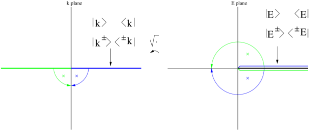
Figure 1: The boundary values of the Lippmann-Schwinger and of the “free” bras and kets.

The analytic continuation of $\chi^{\pm}(r;E)$ is obtained in two steps. First, one specifies the boundary values of the Lippmann-Schwinger eigenfunctions on the upper rim of the cut. And second, one continues those boundary values into the whole two-sheeted Riemann surface, see Fig. 1. The boundary values of the Lippmann-Schwinger eigenfunctions on the upper rim are given by Eq. (2.4).

Because the $\chi^{\pm}(r;E)$ depend explicitly on $k$ rather than on $E$, the analytic continuation of the Lippmann-Schwinger eigenfunctions is more easily obtained in terms of $k$, i.e., in terms of the eigenfunctions $\chi^{\pm}(r;k)$. The $E$-continuation described above translates into a $k$-continuation as follows. First, one specifies the boundary values that the Lippmann-Schwinger eigenfunctions take on the positive $k$-axis. And second, one continues those boundary values into the whole $k$-plane. Since the boundary values of the Lippmann-Schwinger eigenfunctions on the positive $k$-axis are given by Eq. (2.6), and since $\chi^{\pm}(r;k)$ are expressed in terms of well-known analytic functions, the continuation of $\chi^{\pm}(r;k)$ from the positive $k$-axis into the whole wave-number plane is well defined.

Obviously, the analytic continuation of the “free” eigenfunctions $\chi_{0}(r;k)$ follows the same procedure.

A word on notation. Whenever they become complex, we shall denote the energy $E$ and the wave number $k$ by respectively $z$ and $q$. Accordingly, the continuations of $\chi^{\pm}(r;E)$, $\chi_{0}(r;E)$ and $\chi^{\pm}(r;k)$, $\chi_{0}(r;k)$ will be denoted by $\chi^{\pm}(r;z)$, $\chi_{0}(r;z)$ and $\chi^{\pm}(r;q)$, $\chi_{0}(r;q)$. In bra-ket notation, the analytically continued eigenfunctions will be written as

$$\langle r|q^{\pm}\rangle=\chi^{\pm}(r;q)\,,$$ (2.9klmvxyza)

$$\langle^{\pm}q|r\rangle=\chi^{\mp}(r;q)\,,$$ (2.9klmvxyzb)

$$\langle r|q\rangle=\chi_{0}(r;q)\,,$$ (2.9klmvxyzc)

$$\langle q|r\rangle=\chi_{0}(r;q)\,.$$ (2.9klmvxyzd)

In appendix A, we list several useful relations satisfied by these analytically continued eigenfunctions.

In doing analytic continuations, it is important to keep in mind that the combined operations of analytic continuation and complex conjugation do not commute (and also differ in whether the resulting function is analytic or not). The reason lies in the fact that if $f(z)$ is an analytic function, then $\overline{f(z)}$ is not an analytic function. This is why the analytic continuation of $\overline{f(E)}$ must in general be written as $\overline{f(\overline{z})}$. For example, for real wave numbers it holds that

$$\chi^{+}(r;k)=\overline{\chi^{-}(r;k)}\,.$$ (2.9klmvxyze)

When we analytically continue Eq. (2.9klmvxyze), we must write

$$\chi^{+}(r;q)=\overline{\chi^{-}(r;\overline{q})}\,,$$ (2.9klmvxyzf)

rather than

$$\chi^{+}(r;q)=\overline{\chi^{-}(r;q)}\,,$$ (2.9klmvxyzg)

since $\overline{\chi^{-}(r;q)}$ is not analytic. What is more, Eq. (2.9klmvxyzg) is false.

We now turn to characterize the analytic and the growth properties of $\chi^{\pm}(r;q)$. Such properties will be needed in the next section. In order to characterize the analytic properties of $\chi^{\pm}(r;q)$, we define the following sets:

$$Z_{\pm}=\{q\in{\mathbb{C}}\,|\ {\cal J}_{\pm}(q)=0\}\,.$$ (2.9klmvxyzh)

The set $Z_{\pm}$ contains the zeros of the Jost function ${\cal J}_{\pm}(q)$. Because of Eq. (2.9klmvxyzcbxhk), a wave number $q$ belongs to $Z_{+}$ if, and only if, $-q$ belongs to $Z_{-}$. The elements of $Z_{+}$ are simply the discrete, denumerable poles of the $S$ matrix. Since $\chi(r;q)$ and ${\cal J}_{\pm}(q)$ are analytic in the whole $k$-plane [2, 14], $\chi^{\pm}(r;q)$ is analytic in the whole $k$-plane except at $Z_{\pm}$, where its poles are located.

In order to characterize the growth of $\chi^{\pm}(r;q)$, we study first the growth of $\chi(r;q)$. The growth of $\chi(r;q)$ is bounded by the following estimate (see, for example, Eq. (12.6) in Ref. [14]):

$$\left|\chi(r;q)\right|\leq C\,\frac{\left|q\right|r}{1+\left|q\right|r}\,\rme^{|{\rm Im}(q)|r}\,,\quad q\in{\mathbb{C}}\,.$$ (2.9klmvxyzi)

From Eqs. (2.6) and (2.9klmvxyzi), it follows that the eigenfunctions $\chi^{\pm}(r;q)$ satisfy

$$\hskip-28.45274pt\left|\chi^{\pm}(r;q)\right|\leq\frac{C}{|{\cal J}_{\pm}(q)|}\,\frac{|q|r}{1+|q|r}\,\rme^{|{\rm Im}(q)|r}\,.$$ (2.9klmvxyzj)

When $q\in Z_{\pm}$, the Lippmann-Schwinger eigenfunction $\chi^{\pm}(r;q)$ blows up to infinity.

We can further refine the estimates (2.9klmvxyzj) by characterizing the growth of $1/|{\cal J}_{\pm}(q)|$ in different regions of the complex plane. The following proposition, which is based on well-known results [14, 2], and whose proof can be found in appendix B, characterizes the growth of $1/|{\cal J}_{\pm}(q)|$ in different regions of the $k$-plane for the spherical shell potential:

Proposition 1.

The inverse of the Jost function ${\cal J}_{+}(q)$ is bounded in the upper half of the complex wave-number plane:

$$\frac{1}{\left|{\cal J}_{+}(q)\right|}\leq C\,,\quad{\rm Im}(q)\geq 0\,.$$ (2.9klmvxyzk)

In the lower half-plane, $\frac{1}{{\cal J}_{+}(q)}$ is infinite whenever $q\in Z_{+}$. As $|q|$ tends to $\infty$ in the lower half plane, we have

$$\frac{1}{{\cal J}_{+}(q)}\approx\frac{1}{1-Cq^{-2}\rme^{2\rmi qb}}\equiv\frac{1}{\lambda(q)}\,,\quad(|q|\to\infty\,,\ {\rm Im}(q)<0)\,.$$ (2.9klmvxyzl)

The above estimates are satisfied by ${\cal J}_{-}(q)$ when we exchange the upper for the lower half plane, and $Z_{+}$ for $Z_{-}$:

$$\frac{1}{\left|{\cal J}_{-}(q)\right|}\leq C\,,\quad{\rm Im}(q)\leq 0\,.$$ (2.9klmvxyzm)

$$\frac{1}{{\cal J}_{-}(q)}\approx\frac{1}{1-Cq^{-2}\rme^{-2\rmi qb}}\equiv\frac{1}{\lambda(-q)}\,,\quad(|q|\to\infty\,,\ {\rm Im}(q)>0)\,.$$ (2.9klmvxyzn)

Equation (2.9klmvxyzj) and Proposition 1 imply, in particular, that the growth of the “out” eigenfunction in the lower half plane is limited by

$$\left|\chi^{-}(r;q)\right|\leq C\,\frac{\left|q\right|r}{1+\left|q\right|r}\,\rme^{|{\rm Im}(q)|r}\,,\quad{\rm Im}(q)\leq 0\,.$$ (2.9klmvxyzo)

To finish this section, we recall that the “free” eigenfunctions are analytic in the whole complex plane and satisfy an estimate similar to that in Eq. (2.9klmvxyzi), as shown by Eq. (12.4) in Ref. [14]:

$$|\chi_{0}(r;q)|=|\sqrt{2/\pi\,}\sin(qr)|\leq C\frac{|q|r}{1+|q|r}\,\rme^{|{\rm Im}(q)|r}\,,\quad q\in{\mathbb{C}}\,.$$ (2.9klmvxyzp)

4 The analytic continuation of the Lippmann-Schwinger bras and kets

The analytic continuation of the Lippmann-Schwinger bras (2.9kla) is defined for any complex wave number $q$ in the distributional way:

$$\begin{array}[]{rcl}\langle^{\pm}q|:{\mathbf{\Phi}}_{\rm exp}&\longmapsto&{\mathbb{C}}\\ \varphi^{\pm}&\longmapsto&\langle^{\pm}q|\varphi^{\pm}\rangle=\int_{0}^{\infty}\rmd r\,\varphi^{\pm}(r)\chi^{\mp}(r;q)\,,\end{array}$$ (2.9klmvxyza)

where the functions $\varphi^{\pm}(r)$ belong to a space of test functions ${\mathbf{\Phi}}_{\rm exp}$ that will be constructed in the next section. In the bra-ket notation, Eq. (2.9klmvxyza) can be recast as

$$\langle^{\pm}q|\varphi^{\pm}\rangle=\int_{0}^{\infty}\rmd r\,\langle^{\pm}q|r\rangle\langle r|\varphi^{\pm}\rangle\,.$$ (2.9klmvxyzb)

Obviously, when the complex wave number $q$ tends to the real, positive wave number $k$, the bras $\langle^{\pm}q|$ tend to the bras $\langle^{\pm}k|$.

Similarly to the bras (2.9kla), the analytic continuation of the Lippmann-Schwinger kets (2.9klb) is defined as

$$\begin{array}[]{rcl}|q^{\pm}\rangle:{\mathbf{\Phi}}_{\rm exp}&\longmapsto&{\mathbb{C}}\\ \varphi^{\pm}&\longmapsto&\langle\varphi^{\pm}|q^{\pm}\rangle=\int_{0}^{\infty}\rmd r\,\overline{\varphi^{\pm}(r)}\chi^{\pm}(r;q)\,,\end{array}$$ (2.9klmvxyzc)

which in bra-ket notation becomes

$$\langle\varphi^{\pm}|q^{\pm}\rangle=\int_{0}^{\infty}\rmd r\,\langle\varphi^{\pm}|r\rangle\langle r|q^{\pm}\rangle\,.$$ (2.9klmvxyzd)

By construction, when $q$ tends to $k$, the kets $|q^{\pm}\rangle$ tend to the kets $|k^{\pm}\rangle$.

The bras (2.9klmvxyza) and kets (2.9klmvxyzc) are defined for all complex $q$ except at those $q$ at which the corresponding eigenfunction has a pole. Hence, $\langle^{-}q|$ and $|q^{+}\rangle$ are defined everywhere except in $Z_{+}$, whereas $\langle^{+}q|$ and $|q^{-}\rangle$ are defined everywhere except in $Z_{-}$. At those poles, one can still define bras and kets if in definitions (2.9klmvxyza) and (2.9klmvxyzc) one substitutes the eigenfunctions $\chi^{\pm}(r;q)$ by their residues at the pole:

$$\begin{array}[]{rcl}\langle^{\pm}q|:{\mathbf{\Phi}}_{\rm exp}&\longmapsto&{\mathbb{C}}\\ \varphi^{\pm}&\longmapsto&\langle^{\pm}q|\varphi^{\pm}\rangle=\int_{0}^{\infty}\rmd r\,\varphi^{\pm}(r)\,{\rm res}[\chi^{\mp}(r;q)]\,,\quad q\in Z_{\mp}\,,\end{array}$$ (2.9klmvxyze)

$$\begin{array}[]{rcl}|q^{\pm}\rangle:{\mathbf{\Phi}}_{\rm exp}&\longmapsto&{\mathbb{C}}\\ \varphi^{\pm}&\longmapsto&\langle\varphi^{\pm}|q^{\pm}\rangle=\int_{0}^{\infty}\rmd r\,\overline{\varphi^{\pm}(r)}\,{\rm res}[\chi^{\pm}(r;q)]\,,\quad q\in Z_{\pm}\,.\end{array}$$ (2.9klmvxyzf)

In this way, one can associate bras $\langle^{\pm}q|$ and kets $|q^{\pm}\rangle$ with every complex wave number $q$.

The analytic continuation of the “free” bras and kets (2.9klmvxya) and (2.9klmvxyb) into any complex wave number $q$ is defined in the obvious way:

$$\langle q|\varphi\rangle=\int_{0}^{\infty}\rmd r\,\langle q|r\rangle\langle r|\varphi\rangle\int_{0}^{\infty}\rmd r\,\varphi(r)\chi_{0}(r;q)\,,\qquad q\in{\mathbb{C}}\,,$$ (2.9klmvxyzg)

$$\langle\varphi|q\rangle=\int_{0}^{\infty}\rmd r\,\langle\varphi|r\rangle\langle r|q\rangle=\int_{0}^{\infty}\rmd r\,\overline{\varphi(r)}\chi_{0}(r;q)\,,\quad q\in{\mathbb{C}}\,,$$ (2.9klmvxyzh)

where $\varphi$ denotes any asymptotically free wave function. Likewise definitions (2.9klmvxyza) and (2.9klmvxyzc), definitions (2.9klmvxyzg) and (2.9klmvxyzh) make sense when $\varphi$ belongs to ${\mathbf{\Phi}}_{\rm exp}$.

From the analytic continuation of the bras and kets into any complex wave number, one can now obtain the analytic continuation of the bras and kets into any complex energy of the Riemann surface:

$$\begin{array}[]{ccc}|z^{\pm}\rangle=\sqrt{\frac{2m}{\hbar^{2}}\frac{1}{2q}}\,|q^{\pm}\rangle\,,&&\langle^{\pm}z|=\sqrt{\frac{2m}{\hbar^{2}}\frac{1}{2q}}\,\langle^{\pm}q|\,,\\[12.91663pt] |z\rangle=\sqrt{\frac{2m}{\hbar^{2}}\frac{1}{2q}}\,|q\rangle\,,&&\langle z|=\sqrt{\frac{2m}{\hbar^{2}}\frac{1}{2q}}\,\langle q|\,.\end{array}$$ (2.9klmvxyzi)

5 Construction of the rigged Hilbert space for the analytic continuation of the Lippmann-Schwinger bras and kets

Likewise the bras and kets associated with real energies, the analytic continuation of the Lippmann-Schwinger bras and kets must be described within the rigged Hilbert space rather than just within the Hilbert space. We shall denote the rigged Hilbert space for the analytically continued bras by

$${\mathbf{\Phi}}_{\rm exp}\subset L^{2}([0,\infty),\rmd r)\subset{\mathbf{\Phi}}_{\rm exp}^{\prime}\,,$$ (2.9klmvxyza)

and the one for the analytically continued kets by

$${\mathbf{\Phi}}_{\rm exp}\subset L^{2}([0,\infty),\rmd r)\subset{\mathbf{\Phi}}_{\rm exp}^{\times}\,.$$ (2.9klmvxyzb)

In principle, we should construct the space of test functions separately for the “in” and for the “out” wave functions. But since they turn out to be the same, we present the construction for both cases at once.

The functions $\varphi^{\pm}\in{\mathbf{\Phi}}_{\rm exp}$ must satisfy the following conditions:

$$\hskip-11.38092pt\begin{array}[]{lc}&\bullet\ \mbox{They belong to the maximal invariant subspace $\cal D$ of}\ H,\\[4.30554pt] &{\cal D}=\bigcap_{n=0}^{\infty}{\cal D}(H^{n})\,.\end{array}$$ (2.9klmvxyzcc)

$$\bullet\ \mbox{They are such that definitions~{}(\ref{LSdefinitionbra+-q}) and (\ref{LSdefinitionket+-q}) make sense.}$$ (2.9klmvxyzcd)

The reason why $\varphi^{\pm}$ must satisfy condition (2.9klmvxyzcc) is that such condition guarantees that all the powers of the Hamiltonian are well defined. Condition (2.9klmvxyzcc), however, is not sufficient to obtain well-defined bras and kets associated with complex wave numbers. In order for $\langle^{\pm}q|$ and $|q^{\pm}\rangle$ to be well defined, the wave functions $\varphi^{\pm}(r)$ must be well behaved so the integrals in Eqs. (2.9klmvxyza) and (2.9klmvxyzc) converge. How well $\varphi^{\pm}(r)$ must behave is determined by how bad $\chi^{\pm}(r;q)$ behave. Since by Eq. (2.9klmvxyzj) $\chi^{\pm}(r;q)$ grow exponentially with $r$, the wave functions $\varphi^{\pm}(r)$ have to, essentially, tame real exponentials. If we define

$$\hskip-56.9055pt\|\varphi^{\pm}\|_{n,n^{\prime}}:=\sqrt{\int_{0}^{\infty}\rmd r\,\left|\frac{nr}{1+nr}\,\rme^{nr^{2}/2}(1+H)^{n^{\prime}}\varphi^{\pm}(r)\right|^{2}\,}\,,\quad n,n^{\prime}=0,1,2,\ldots\,,$$ (2.9klmvxyzcd)

then the space ${\mathbf{\Phi}}_{\rm exp}$ is given by

$${\mathbf{\Phi}}_{\rm exp}=\left\{\varphi^{\pm}\in{\cal D}\,|\ \|\varphi^{\pm}\|_{n,n^{\prime}}<\infty\,,\ n,n^{\prime}=0,1,2,\ldots\right\}.$$ (2.9klmvxyzce)

This is just the space of square integrable functions which belong to the maximal invariant subspace of $H$ and for which the quantities (2.9klmvxyzcd) are finite. In particular, because $\varphi^{\pm}(r)$ satisfy the estimates (2.9klmvxyzcd), $\varphi^{\pm}(r)$ fall off at infinity faster than $\rme^{-r^{2}}$, that is, their tails fall off faster than Gaussians.

From Eq. (2.9klmvxyzj), it is clear that the integrals in Eqs. (2.9klmvxyza) and (2.9klmvxyzc) converge already for functions that fall off at infinity faster than any exponential. We have imposed Gaussian falloff because it allows us to perform expansions in terms of the Gamow states, as will be discussed elsewhere.

It is illuminating to compare the space of test functions needed to accommodate the Lippmann-Schwinger bras and kets associated with real wave numbers, the space $\mathbf{\Phi}$ of Ref. [1], with the space of test functions needed to accommodate their analytic continuation, the space ${\mathbf{\Phi}}_{\rm exp}$ of Eq. (2.9klmvxyzce). Because for real wave numbers the Lippmann-Schwinger eigenfunctions behave like purely imaginary exponentials, in this case we only need to impose on the test functions a polynomial falloff, thereby obtaining a space of test functions very similar to the Schwartz space. By contrast, for complex wave numbers the Lippmann-Schwinger eigenfunctions blow up exponentially, and therefore we need to impose on the test functions an exponential falloff that damps such an exponential blowup.

The quantities (2.9klmvxyzcd) are norms, and they can be used to define a countably normed topology (i.e., a meaning of sequence convergence) $\tau_{\mathbf{\Phi}_{\rm exp}}$ on $\mathbf{\Phi}_{\rm exp}$:

$$\varphi^{\pm}_{\alpha}\,\smash{\mathop{\relbar\joinrel\longrightarrow}\limits^{\tau_{\mathbf{\Phi}_{\rm exp}}}_{\alpha\to\infty}}\,\varphi^{\pm}\quad{\rm iff}\quad\|\varphi^{\pm}_{\alpha}-\varphi^{\pm}\|_{n,n^{\prime}}\,\smash{\mathop{\relbar\joinrel\longrightarrow}\limits_{\alpha\to\infty}}\,0\,,\quad n,n^{\prime}=0,1,2,\ldots\,.$$ (2.9klmvxyzcf)

Once we have constructed the space $\mathbf{\Phi}_{\rm exp}$, we can construct its dual $\mathbf{\Phi}_{\rm exp}^{\prime}$ and antidual $\mathbf{\Phi}_{\rm exp}^{\times}$ spaces as the spaces of, respectively, linear and antilinear continuous functionals over $\mathbf{\Phi}_{\rm exp}$, and therewith the rigged Hilbert spaces (2.9klmvxyza) and (2.9klmvxyzb). The Lippmann-Schwinger bras and kets are, respectively, linear and antilinear continuous functionals over ${\mathbf{\Phi}}_{\rm exp}$, i.e., $\langle^{\pm}q|\in{\mathbf{\Phi}}_{\rm exp}^{\prime}$ and $|q^{\pm}\rangle\in{\mathbf{\Phi}}_{\rm exp}^{\times}$. As well, $\langle^{\pm}q|$ and $|q^{\pm}\rangle$ are, respectively, “left” and “right” eigenvectors of $H$ with eigenvalue $\hbar^{2}/(2m)\,q^{2}$.

The following proposition, whose proof can be found in appendix B, encapsulates the results of this section:

Proposition 2.

The triplets of spaces (2.9klmvxyza) and (2.9klmvxyzb) are rigged Hilbert spaces, and they satisfy all the requirements to accommodate the analytic continuation of the Lippmann-Schwinger bras and kets. More specifically,

• The $\|\cdot\|_{n,n^{\prime}}$ are norms.

• The space ${\mathbf{\Phi}}_{\rm exp}$ is dense in $L^{2}([0,\infty),\rmd r)$.

• The space ${\mathbf{\Phi}}_{\rm exp}$ is invariant under the action of the Hamiltonian, and $H$ is ${\mathbf{\Phi}_{\rm exp}}$-continuous.

• The kets $|q^{\pm}\rangle$ are continuous, antilinear functionals over ${\mathbf{\Phi}}_{\rm exp}$, i.e., $|q^{\pm}\rangle\in{\mathbf{\Phi}}_{\rm exp}^{\times}$.

• The kets $|q^{\pm}\rangle$ are “right” eigenvectors of $H$ with eigenvalue $\frac{\hbar^{2}}{2m}q^{2}$:

  $$H|q^{\pm}\rangle=\frac{\hbar^{2}}{2m}q^{2}\,|q^{\pm}\rangle\,;$$ (2.9klmvxyzcga)

  that is,

  $$\langle\varphi^{\pm}|H|q^{\pm}\rangle=\frac{\hbar^{2}}{2m}q^{2}\langle\varphi^{\pm}|H|q^{\pm}\rangle\,,\quad\varphi^{\pm}\in{\mathbf{\Phi}}_{\rm exp}\,.$$ (2.9klmvxyzcgb)

• The bras $\langle^{\pm}q|$ are continuous, linear functionals over ${\mathbf{\Phi}}_{\rm exp}$, i.e., $\langle^{\pm}q|\in{\mathbf{\Phi}}_{\rm exp}^{\prime}$.

• The bras $\langle^{\pm}q|$ are “left” eigenvectors of $H$ with eigenvalue $\frac{\hbar^{2}}{2m}q^{2}$:

  $$\langle^{\pm}q|H=\frac{\hbar^{2}}{2m}q^{2}\langle^{\pm}q|\,;$$ (2.9klmvxyzcgha)

  that is,

  $$\langle^{\pm}q|H|\varphi^{\pm}\rangle=\frac{\hbar^{2}}{2m}q^{2}\langle^{\pm}q|\varphi^{\pm}\rangle\,.$$ (2.9klmvxyzcghb)

Equations (2.9klmvxyzcga) and (2.9klmvxyzcgha) can be rewritten in terms of the complex energy $z$ as

$$H|z^{\pm}\rangle=z|z^{\pm}\rangle\,,$$ (2.9klmvxyzci)

$$\langle^{\pm}z|H=z\langle^{\pm}z|\,.$$ (2.9klmvxyzcj)

Note that the bra eigenequation (2.9klmvxyzcj) is not given by $\langle^{\pm}z|H=\overline{z}\langle^{\pm}z|$, as one may naively expect from formally obtaining (2.9klmvxyzcj) by Hermitian conjugation of the ket eigenequation (2.9klmvxyzci). The reason lies in that the function $\overline{z}$ is not analytic, so when one obtains the bra eigenequation by Hermitian conjugation of the ket eigenequation, one has to use $\overline{\overline{z}}=z$. The following chain of equalities further clarifies this point:

$$\langle^{\pm}z|H|\varphi^{\pm}\rangle=z\langle^{\pm}z|\varphi^{\pm}\rangle=z\overline{\langle\varphi^{\pm}|\overline{z}^{\pm}\rangle}=\overline{\overline{z}\langle\varphi^{\pm}|\overline{z}^{\pm}\rangle}=\overline{\langle\varphi^{\pm}|H|\overline{z}^{\pm}\rangle}\,.$$ (2.9klmvxyzck)

The “free” bras (2.9klmvxyzg) and kets (2.9klmvxyzh) can also be accommodated within the rigged Hilbert spaces (2.9klmvxyza) and (2.9klmvxyzb). To see this, one just has to recall the estimate (2.9klmvxyzp). One can then show, in complete analogy with the Lippmann-Schwinger bras and kets, that $\langle q|$ belongs to ${\mathbf{\Phi}}_{\rm exp}^{\prime}$, and that $|q\rangle$ belongs to ${\mathbf{\Phi}}_{\rm exp}^{\times}$. As well, one can easily prove that $\langle q|$ and $|q\rangle$ are, respectively, “left” and “right” eigenvectors of $H_{0}$ with eigenvalue $\frac{\hbar^{2}}{2m}q^{2}$.

It is clear that there is a 1:1 correspondence between bras and kets also when the energy and the wave number become complex. The following table summarizes such correspondence:

wave number $$\longleftrightarrow$$ energy

bra ,   ,  

ket ,   ,  

(2.9klmvxyzcl)

6 The wave number representations of the rigged Hilbert spaces, bras and kets

We turn now to obtain and characterize the wave number representations of the rigged Hilbert spaces (2.9klmvxyza) and (2.9klmvxyzb) as well as of the “in” and “out” wave functions, bras and kets. The wave number representations are very useful, because sometimes they differentiate between the “in” and the “out” boundary conditions in a more clear way than the position representation.

6.1 The wave number representations of the rigged Hilbert spaces

The “in” ($+$) and the “out” ($-$) wave number representations of ${\mathbf{\Phi}}_{\rm exp}$ are readily obtained by means of the unitary operators ${\cal F}_{\pm}$ of Eq. (2.9j):

$${\cal F}_{\pm}{\mathbf{\Phi}}_{\rm exp}\equiv\widehat{\mathbf{\Phi}}_{\pm{\rm exp}}\,,$$ (2.9klmvxyzca)

which in turn yield the wave number representations of the rigged Hilbert spaces (2.9klmvxyza) and (2.9klmvxyzb):

$$\widehat{\mathbf{\Phi}}_{\pm{\rm exp}}\subset L^{2}([0,\infty),\rmd k)\subset\widehat{\mathbf{\Phi}}_{\pm{\rm exp}}^{\prime}\,,$$ (2.9klmvxyzcba)

$$\widehat{\mathbf{\Phi}}_{\pm{\rm exp}}\subset L^{2}([0,\infty),\rmd k)\subset\widehat{\mathbf{\Phi}}_{\pm{\rm exp}}^{\times}\,.$$ (2.9klmvxyzcbb)

The functions $\widehat{\varphi}^{\pm}(q)$ in $\widehat{\mathbf{\Phi}}_{\pm{\rm exp}}$ are obviously the analytic continuation of $\widehat{\varphi}^{\pm}(k)$ from the positive $k$-axis into the whole $k$-plane. One can easily show that

$$\widehat{\varphi}^{\pm}(q)=\langle^{\pm}q|\varphi^{\pm}\rangle\,,$$ (2.9klmvxyzcbc)

and that

$$\overline{\widehat{\varphi}^{\pm}(\overline{q})}=\langle\varphi^{\pm}|q^{\pm}\rangle\,.$$ (2.9klmvxyzcbd)

The poles of the Lippmann-Schwinger eigenfunctions are carried over into the analytic continuation of the wave functions: The function $\widehat{\varphi}^{\pm}(q)$ is analytic everywhere except at $Z_{\mp}$, where its poles are located, and $\overline{\widehat{\varphi}^{\pm}(\overline{q})}$ is analytic everywhere except at $Z_{\pm}$, where its poles are located.

That $\widehat{\varphi}^{\pm}(k)$ can be analytically continued into $\widehat{\varphi}^{\pm}(q)$ is made possible by the falloff of $\varphi^{\pm}(r)$ at infinity. The falloff of $\varphi^{\pm}(r)$ also limits the growth of $\widehat{\varphi}^{\pm}(q)$. Such growth is provided by the following proposition:

Proposition 3.

In the lower half of the $k$-plane, $\widehat{\varphi}^{+}(q)$ grows slower than $\rme^{|{\rm Im}(q)|^{2}}$. More precisely, for every positive integer $n^{\prime}$, and for each $\alpha>0$, the following estimate holds:

$$|(1+\frac{\hbar^{2}}{2m}q^{2})^{n^{\prime}}\widehat{\varphi}^{+}(q)|\leq C\,\rme^{\frac{\,\,|{\rm Im}(q)|^{2}}{2\alpha}}\,,\quad{\rm Im}(q)\leq 0\,,$$ (2.9klmvxyzcbe)

where the constant $C$ depends on ${n^{\prime}}$, ${\varphi}^{+}$ and $\alpha$, but not on $q$. In the upper half plane, $\widehat{\varphi}^{+}(q)$ is infinity whenever $q\in Z_{-}$. As $|q|$ tends to $\infty$ in the upper half plane, it holds that

$$|(1+\frac{\hbar^{2}}{2m}q^{2})^{n^{\prime}}\widehat{\varphi}^{+}(q)|\leq C\,\frac{1}{|\lambda(-q)|}\rme^{\frac{\,\,|{\rm Im}(q)|^{2}}{2\alpha}}\,,\quad(|q|\to\infty\,,\ {\rm Im}(q)>0)\,,$$ (2.9klmvxyzcbf)

where $\lambda(-q)$ is given by Proposition 1.

The above estimates are satisfied by $\widehat{\varphi}^{-}(q)$ when we exchange the upper for the lower half plane:

$$|(1+\frac{\hbar^{2}}{2m}q^{2})^{n^{\prime}}\widehat{\varphi}^{-}(q)|\leq C\,\rme^{\frac{\,\,|{\rm Im}(q)|^{2}}{2\alpha}}\,,\quad{\rm Im}(q)\geq 0\,.$$ (2.9klmvxyzcbg)

$$|(1+\frac{\hbar^{2}}{2m}q^{2})^{n^{\prime}}\widehat{\varphi}^{-}(q)|\leq C\,\frac{1}{|\lambda(q)|}\rme^{\frac{\,\,|{\rm Im}(q)|^{2}}{2\alpha}}\,,\quad(|q|\to\infty\,,\ {\rm Im}(q)<0)\,,$$ (2.9klmvxyzcbh)

The proof of Proposition 3 can be found in appendix B, and it is based on the theory of $M$ and $\Omega$ functions, see Ref. [12] and appendix C. For our purposes, the most important result is

$$xy\leq\frac{x^{n}}{n}+\frac{y^{n^{\prime}}}{n^{\prime}}\,,$$ (2.9klmvxyzcbi)

where $x,y\geq 0$ and

$$\frac{1}{n}+\frac{1}{n^{\prime}}=1\,.$$ (2.9klmvxyzcbj)

Equation (2.9klmvxyzcbi) can be used to show that when $\varphi^{\pm}(r)$ falls off faster than $\rme^{-r^{n}}$, then, away from its poles, $\widehat{\varphi}^{\pm}(q)$ grows slower than $\rme^{|{\rm Im}(q)|^{n^{\prime}}}$. In this paper, we use $n=n^{\prime}=2$.

The bounds in Proposition 3 are very wasteful when $|q|\to 0$, where $\widehat{\varphi}^{\pm}(q)$ actually tends to $0$. This happened because in the proof of Proposition 3, we dismiss the factor $|q|r/(1+|q|r)$. Dismissing this factor should not be the cause of concern, since the most crucial behavior of $\widehat{\varphi}^{\pm}(q)$ occurs in the limit $|q|\to\infty$.

It is interesting to compare the growth of our test functions with the growth of the test functions used by Bollini et al. [10, 11]. In [10, 11], $\varphi(r)$ falls off like $\rme^{-r}$, and therefore $|\widehat{\varphi}(p)|$ grows faster than any exponential of $|{\rm Im}(p)|^{n}$, where $p$ denotes the complex momentum and $n$ can be any positive integer. In the present paper, $\varphi(r)$ falls off like $\rme^{-r^{2}}$, and therefore $|\widehat{\varphi}^{\pm}(q)|$ grows like $\rme^{|{\rm Im}(q)|^{2}}$ away from its poles.

It is also interesting to compare our approach with that based on Hardy functions [3, 4, 5, 6, 7, 8, 9]. From Eq. (2.8), one can obtain the analytic and growth properties of the wave functions in the energy representation, $\widehat{\varphi}^{\pm}(z)$, from those of $\widehat{\varphi}^{\pm}(q)$. Since by Proposition 3 the wave functions $\widehat{\varphi}^{\pm}(q)$ blow up exponentially in the infinity arc of the wave number plane, the wave functions $\widehat{\varphi}^{\pm}(z)$ also blow up exponentially in the infinity arcs of the Riemann surface. Therefore, $\widehat{\varphi}^{\pm}(z)$ are not Hardy functions, because if they were, they would tend to zero in one of the infinite semi-arcs of the Riemann surface. Hence, our approach is different from that based on Hardy functions.

6.2 The wave number representation of the Lippmann-Schwinger bras and kets

The wave number representation of the bras $\langle^{\pm}q|$ and kets $|q^{\pm}\rangle$ is defined as

$$\langle^{\pm}\widehat{q}|\equiv\langle^{\pm}q|{\cal F}_{\pm}\,,$$ (2.9klmvxyzcbk)

$$|\widehat{q}^{\pm}\rangle\equiv{\cal F}_{\pm}|q^{\pm}\rangle\,.$$ (2.9klmvxyzcbl)

The bras $\langle^{\pm}q|$ and kets $|q^{\pm}\rangle$ are obviously different from their wave-number representations $\langle^{\pm}\widehat{q}|$ and $|\widehat{q}^{\pm}\rangle$, and such difference can be better understood through a simpler example. Consider the 1D momentum operator $P=-\rmi\hbar\rmd/\rmd x$. In the position representation, the $\delta$-normalized eigenfunctions of $P$ are the exponentials $\frac{1}{\sqrt{2\pi\hbar}}\rme^{\rmi px/\hbar}$, and these are the analog of $|q^{\pm}\rangle$. In the momentum representation, which is obtained by Fourier transforming the position representation, the eigenfunctions of the momentum operator become the delta function $\delta(p-p^{\prime})$, and these are the analog of $|\widehat{q}^{\pm}\rangle$.

When $q$ does not belong to $Z_{\mp}$, the bras $\langle^{\pm}\widehat{q}|$ act as the linear complex delta functional, as the following chain of equalities show:

$$\langle^{\pm}\widehat{q}|\widehat{\varphi}^{\pm}\rangle =\langle^{\pm}q|{\cal F}_{\pm}|\widehat{\varphi}^{\pm}\rangle$$ by (2.9klmvxyzcbk) (2.9klmvxyzcbm)

$$=\langle^{\pm}q|{\cal F}_{\pm}^{\dagger}\widehat{\varphi}^{\pm}\rangle$$ by (2.9klmvxyzcbxha)

$$=\langle^{\pm}q|{\varphi}^{\pm}\rangle$$

$$=\widehat{\varphi}^{\pm}(q)\,,\quad q\notin Z_{\mp} \hskip 28.45274pt\mbox{by (\ref{expreofbraintwf})}\,.$$

When $q$ belongs to $Z_{\mp}$, the wave function $\widehat{\varphi}^{\pm}(q)$ has a pole at $q$, and therefore the bra $\langle^{\pm}\widehat{q}|$ acts as the linear residue functional:

$$\langle^{\pm}\widehat{q}|\widehat{\varphi}^{\pm}\rangle={\rm res}\,[\widehat{\varphi}^{\pm}(q)]\,,\quad q\in Z_{\mp}\,.$$ (2.9klmvxyzcbn)

Similarly, when $q$ does not belong to $Z_{\pm}$, the kets $|q^{\pm}\rangle$ act as the antilinear complex delta functional, as the following chain of equalities show:

$$\langle\widehat{\varphi}^{\pm}|\widehat{q}^{\pm}\rangle =\langle\widehat{\varphi}^{\pm}|{\cal F}_{\pm}|q^{\pm}\rangle$$ by (2.9klmvxyzcbl) (2.9klmvxyzcbo)

$$=\langle{\cal F}_{\pm}^{\dagger}\widehat{\varphi}^{\pm}|q^{\pm}\rangle$$ by (2.9klmvxyzcbxhb)

$$=\langle\varphi^{\pm}|q^{\pm}\rangle$$

$$=\overline{\widehat{\varphi}^{\pm}(\overline{q})}\,,\quad q\notin Z_{\pm} \hskip 28.45274pt\mbox{by (\ref{expreofketintwf})}\,.$$

When $q$ belongs to $Z_{\pm}$, the wave function $\overline{\widehat{\varphi}^{\pm}(\overline{q})}$ has a pole at $q$, and therefore the ket $|q^{\pm}\rangle$ acts as the antilinear residue functional:

$$\langle\widehat{\varphi}^{\pm}|\widehat{q}^{\pm}\rangle={\rm res}\,[\overline{\widehat{\varphi}^{\pm}(\overline{q})}]\,,\quad q\in Z_{\pm}\,.$$ (2.9klmvxyzcbp)

The complex delta functional and the residue functional can be written in more familiar terms as follows. By using the resolution of the identity (2.9klmn), we can formally write the action of $\langle^{\pm}\widehat{q}|$ as an integral operator and obtain

$$\langle^{\pm}\widehat{q}|\widehat{\varphi}^{\pm}\rangle =\langle^{\pm}q|{\varphi}^{\pm}\rangle$$ (2.9klmvxyzcbq)

$$=\int_{0}^{\infty}\rmd k\,\langle^{\pm}q|k^{\pm}\rangle\langle^{\pm}k|{\varphi}^{\pm}\rangle$$

$$=\int_{0}^{\infty}\rmd k\,\langle^{\pm}q|k^{\pm}\rangle\,\widehat{\varphi}^{\pm}(k)\,.$$

Comparison of (2.9klmvxyzcbq) with (2.9klmvxyzcbm) shows that when $q\notin Z_{\mp}$, $\langle^{\pm}q|k^{\pm}\rangle$ coincides with the complex delta function at $q$:

$$\langle^{\pm}q|k^{\pm}\rangle=\delta(k-q)\,,\quad q\notin Z_{\mp}\,.$$ (2.9klmvxyzcbr)

Note that when $q$ is positive, Eq. (2.9klmvxyzcbr) reduces to the standard $\delta$-function normalization. When $q\in Z_{\mp}$, comparison of (2.9klmvxyzcbq) with (2.9klmvxyzcbn) implies that $\langle^{\pm}q|k^{\pm}\rangle$ coincides with the residue distribution at $q$:

$$\langle^{\pm}q|k^{\pm}\rangle={\rm res}\,[\,\cdot\,]_{q}\,,\quad q\in Z_{\mp}\,.$$ (2.9klmvxyzcbs)

Similarly, by using (2.9klmn) we can formally write the action of $|\widehat{q}^{\pm}\rangle$ as an integral operator:

$$\langle\widehat{\varphi}^{\pm}|\widehat{q}^{\pm}\rangle =\langle{\varphi}^{\pm}|q^{\pm}\rangle$$ (2.9klmvxyzcbt)

$$=\int_{0}^{\infty}\rmd k\,\langle{\varphi}^{\pm}|k^{\pm}\rangle\langle^{\pm}k|q^{\pm}\rangle$$

$$=\int_{0}^{\infty}\rmd k\,\overline{\varphi^{\pm}(k)}\langle^{\pm}k|q^{\pm}\rangle\,.$$

By comparing (2.9klmvxyzcbt) with (2.9klmvxyzcbo), we deduce that when $q\notin Z_{\pm}$, $\langle^{\pm}k|q^{\pm}\rangle$ coincides with the complex delta function at $q$:

$$\langle^{\pm}k|q^{\pm}\rangle=\delta(k-q)\,,\quad q\notin Z_{\pm}\,.$$ (2.9klmvxyzcbu)

When $q\in Z_{\pm}$, comparison of (2.9klmvxyzcbt) with (2.9klmvxyzcbp) lead us to identify $\langle^{\pm}k|q^{\pm}\rangle$ as the residue distribution at $q$:

$$\langle^{\pm}k|q^{\pm}\rangle={\rm res}\,[\,\cdot\,]_{q}\,,\quad q\in Z_{\pm}\,.$$ (2.9klmvxyzcbv)

It is important to note that, with a given test function, the complex delta function and the residue distribution at $q$ associate, respectively, the value and the residue of the analytic continuation of the test function at $q$. This is why when those distributions act on $\overline{\widehat{\varphi}^{\pm}(k)}$ as in Eq. (2.9klmvxyzcbt), the final result is respectively $\overline{\widehat{\varphi}^{\pm}(\overline{q})}$ and ${\rm res}\,[\overline{\widehat{\varphi}^{\pm}(\overline{q})}]$, rather than $\overline{\widehat{\varphi}^{\pm}(q)}$ and ${\rm res}\,[\overline{\widehat{\varphi}^{\pm}(q)}]$, since the analytic continuation of $\overline{\widehat{\varphi}^{\pm}(k)}$ is $\overline{\widehat{\varphi}^{\pm}(\overline{q})}$ rather than $\overline{\widehat{\varphi}^{\pm}(q)}$.

6.3 The “free” wave number representation

One can also construct the wave number representation associated with the “free” Hamiltonian. Since its construction follows the same steps as that of the “in” and “out” wave number representations, we shall simply list the main results.

The unitary operator ${\cal F}_{0}$ in Eq. (2.9klmvw) provides the “free” wave number representation of the space of test functions:

$${\cal F}_{0}{\mathbf{\Phi}}_{\rm exp}\equiv\widehat{\mathbf{\Phi}}_{0{\rm exp}}\,,$$ (2.9klmvxyzcbw)

which in turn yields the “free” wave number representation of the rigged Hilbert spaces (2.9klmvxyza) and (2.9klmvxyzb):

$$\widehat{\mathbf{\Phi}}_{0{\rm exp}}\subset L^{2}([0,\infty),\rmd k)\subset\widehat{\mathbf{\Phi}}_{0{\rm exp}}^{\prime}\,,$$ (2.9klmvxyzcbxa)

$$\widehat{\mathbf{\Phi}}_{0{\rm exp}}\subset L^{2}([0,\infty),\rmd k)\subset\widehat{\mathbf{\Phi}}_{0{\rm exp}}^{\times}\,.$$ (2.9klmvxyzcbxb)

The functions $\widehat{\varphi}(q)$ in $\widehat{\mathbf{\Phi}}_{0{\rm exp}}$ are the analytic continuation of $\widehat{\varphi}(k)$ from the positive $k$-axis into the whole $k$-plane. One can easily show that

$$\widehat{\varphi}(q)=\langle q|\varphi\rangle\,,\quad q\in{\mathbb{C}}\,.$$ (2.9klmvxyzcbxy)

and that

$$\overline{\widehat{\varphi}(\overline{q})}=\langle\varphi|q\rangle\,,\quad q\in{\mathbb{C}}\,.$$ (2.9klmvxyzcbxz)

The functions $\widehat{\varphi}(q)$ are analytic in the whole $k$-plane, and they satisfy the following estimate for any $\alpha>0$ and for any positive integer $n^{\prime}$:

$$|(1+\frac{\hbar^{2}}{2m}q^{2})^{n^{\prime}}\widehat{\varphi}(q)|\leq C\,\rme^{\frac{\,\,|{\rm Im}(q)|^{2}}{2\alpha}}\,,\quad q\in{\mathbb{C}}\,,$$ (2.9klmvxyzcbxaa)

where the constant $C$ depends on ${n^{\prime}}$, ${\varphi}$ and $\alpha$, but not on $q$.

The “free” wave number representation of $\langle q|$ and $|q\rangle$ is defined as

$$\langle\widehat{q}|\equiv\langle q|{\cal F}_{0}\,,$$ (2.9klmvxyzcbxab)

$$|\widehat{q}\rangle\equiv{\cal F}_{0}|q\rangle\,.$$ (2.9klmvxyzcbxac)

One can easily show that $\langle\widehat{q}|$ and $|\widehat{q}\rangle$ are, respectively, the linear and antilinear complex delta functionals.

7 The time evolution of the analytic continuation of the Lippmann-Schwinger bras and kets

In Ref. [1], we obtained the time evolution of the “in,” as well as of the “out,” wave functions, bras and kets. In terms of the wave number, the time evolution of the wave functions $\varphi^{\pm}$ is given by

$$\varphi^{\pm}(r;t)=\left(\rme^{-\rmi Ht/\hbar}\varphi^{\pm}\right)(r)=\int_{0}^{\infty}\rmd k\,\rme^{-\rmi k^{2}\hbar t/(2m)}\widehat{\varphi}^{\pm}(k)\chi^{\pm}(r;k)\,,$$ (2.9klmvxyzcbxa)

which is valid for $-\infty<t<\infty$. Equation (2.9klmvxyzcbxa) is equivalent to saying that the operator $\rme^{-\rmi Ht/\hbar}$ acts, in the wave number representation, as multiplication by $\rme^{-\rmi k^{2}\hbar t/(2m)}$:

$$\widehat{\varphi}^{\pm}(k;t)=\left(\rme^{-\rmi\widehat{H}t/\hbar}\widehat{\varphi}^{\pm}\right)(k)=\rme^{-\rmi k^{2}\hbar t/(2m)}\widehat{\varphi}^{\pm}(k)\,.$$ (2.9klmvxyzcbxb)

For $k$ positive, the time evolution of the Lippmann-Schwinger bras and kets is given by

$$\langle^{\pm}k|\rme^{-\rmi Ht/\hbar}=\rme^{\rmi k^{2}\hbar t/(2m)}\langle^{\pm}k|\,,$$ (2.9klmvxyzcbxc)

$$\rme^{-\rmi Ht/\hbar}|k^{\pm}\rangle=\rme^{-\rmi k^{2}\hbar t/(2m)}|k^{\pm}\rangle\,.$$ (2.9klmvxyzcbxd)

In this section, we analytically continue the above equations into the $k$-plane, thereby obtaining the time evolution of the analytic continuation of the “in,” as well as of the “out,” wave functions, bras and kets. As we shall see, such continuation entails the imposition of a time asymmetric boundary condition upon the time evolution.

7.1 The analytic continuation of the time evolution

The analytic continuation of Eq. (2.9klmvxyzcbxb) is given by

$$\widehat{\varphi}^{\pm}(q;t)=\left(\rme^{-\rmi\widehat{H}t/\hbar}\widehat{\varphi}^{\pm}\right)(q)=\rme^{-\rmi q^{2}\hbar t/(2m)}\widehat{\varphi}^{\pm}(q)\,.$$ (2.9klmvxyzcbxe)

The factor $\rme^{-\rmi q^{2}\hbar t/(2m)}$ does not change the analytic properties of $\widehat{\varphi}^{\pm}(q)$. It does, however, change the growth properties of $\widehat{\varphi}^{\pm}(q)$ depending on the sign of $t$ and on the quadrant of the complex plane. As can be easily seen,

$$\rme^{-\rmi q^{2}\hbar t/(2m)}\smash{\mathop{\relbar\joinrel\longrightarrow}\limits^{\quad}_{\ |q|\to\infty\ }}0\,,\begin{array}[]{c}\quad t>0\,,\ q\in{\rm 2nd,4th},\\ \hskip-11.38092pt{\rm or}\\ \quad t<0\,,\ q\in{\rm 1st,3rd},\end{array}$$ (2.9klmvxyzcbxf)

$$\rme^{-\rmi q^{2}\hbar t/(2m)}\smash{\mathop{\relbar\joinrel\longrightarrow}\limits^{\quad}_{\ |q|\to\infty\ }}\infty\,,\begin{array}[]{c}\quad t<0\,,\ q\in{\rm 2nd,4th},\\ \hskip-11.38092pt{\rm or}\\ \quad t>0\,,\ q\in{\rm 1st,3rd},\end{array}$$ (2.9klmvxyzcbxg)

where 1st, 2nd, 3rd and 4th denote, respectively, the first, second, third and fourth quadrants of the $k$-plane. Thus, even though $\widehat{\varphi}^{\pm}(q)$ blows up exponentially for large $q$, $\widehat{\varphi}^{\pm}(q;t)$ goes to zero in the infinite arc of the second and fourth quadrants when $t>0$. In the infinite arc of the first and third quadrants, $\widehat{\varphi}^{\pm}(q;t)$ goes to zero when $t<0$. Hence, the analytic continuation of the time evolution changes the growth properties of the wave functions and introduces a time asymmetry.

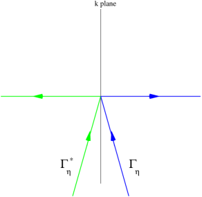
Figure 2: The contours $\Gamma_{\eta}$ and $\Gamma_{\eta}^{*}$. The straight lines in the third and fourth quadrants form an angle $\eta$ with the negative imaginary axis, $\eta$ being infinitesimally small.

In practical situations, the importance of the limits (2.9klmvxyzcbxf) lies in the fact that they enable us to continue certain contour integrals all the way to the infinite arc of a quadrant in such a way that such infinite arc does not contribute to the integral. For example, if $\Gamma_{\eta}$ and $\Gamma_{\eta}^{*}$ denote the contours depicted in Fig. 2, then Cauchy’s theorem and the bound (2.9klmvxyzcbe), together with the limits (2.9klmvxyzcbxf), yield

$$\int_{\Gamma_{\eta}}\rmd q\,\rme^{-\rmi q^{2}\hbar t/(2m)}\widehat{\varphi}^{+}(q)=0\,,\quad t>0\,,$$ (2.9klmvxyzcbxha)

$$\int_{\Gamma_{\eta}^{*}}\rmd q\,\rme^{-\rmi q^{2}\hbar t/(2m)}\widehat{\varphi}^{+}(q)=0\,,\quad t<0\,.$$ (2.9klmvxyzcbxhb)

These two equations exemplify the different behavior of $\widehat{\varphi}^{+}(q;t)$ in different quadrants of the $k$-plane for opposite signs of time.

Our next objective is to analytically continue Eq. (2.9klmvxyzcbxa). In order to do so, we define the contour $\gamma_{\varepsilon}$ as the radial path in the fourth quadrant that forms an angle $-\varepsilon$ with the positive $k$-axis, see Fig. 3a. Then,

$$\varphi^{\pm}(r;t)=\int_{\gamma_{\varepsilon}}\rmd q\,\rme^{-\rmi q^{2}\hbar t/(2m)}\widehat{\varphi}^{\pm}(q)\chi^{\pm}(r;q)\,.$$ (2.9klmvxyzcbxhi)

Because by (2.9klmvxyzcbxf) and (2.9klmvxyzcbxg) $\rme^{-\rmi q^{2}\hbar t/(2m)}$ tends to zero in the infinite arc of the fourth quadrant only for positive times, the time evolution (2.9klmvxyzcbxhi) is defined only for $t>0$. Thus, the analytic continuation into the fourth quadrant converts the time evolution group $\rme^{-\rmi Ht/\hbar}$ into a semigroup. We shall denote this semigroup by $\rme_{+}^{-\rmi Ht/\hbar}$:

$$\hskip-28.45274pt\varphi^{\pm}(r;t)=\left(\rme_{+}^{-\rmi Ht/\hbar}\varphi^{\pm}\right)(r)=\int_{\gamma_{\varepsilon}}\rmd q\,\rme^{-\rmi q^{2}\hbar t/(2m)}\widehat{\varphi}^{\pm}(q)\chi^{\pm}(r;q)\,,\quad t>0\,.$$ (2.9klmvxyzcbxhj)

Similarly, because by (2.9klmvxyzcbxf) and (2.9klmvxyzcbxg) $\rme^{-\rmi q^{2}\hbar t/(2m)}$ tends to zero in the infinite arc of the third quadrant only for negative times, the analytic continuation of the time evolution into the 3rd quadrant converts $\rme^{-\rmi Ht/\hbar}$ into a semigroup valid for $t<0$ only. We shall denote this semigroup by $\rme_{-}^{-\rmi Ht/\hbar}$:

$$\hskip-42.67912pt\varphi^{\pm}(r;t)=\left(\rme_{-}^{-\rmi Ht/\hbar}\varphi^{\pm}\right)(r)=-\int_{\gamma_{\varepsilon}^{*}}\rmd q\,\rme^{-\rmi q^{2}\hbar t/(2m)}\overline{\widehat{\varphi}^{\pm}(\overline{q})}\ \overline{\chi^{\pm}(r;\overline{q})}\,,\quad t<0\,,$$ (2.9klmvxyzcbxhk)

where $\gamma_{\varepsilon}^{*}$ is the mirror image of $\gamma_{\varepsilon}$ with respect to the imaginary axis, see Fig. 3a. In Eqs. (2.9klmvxyzcbxhj) and (2.9klmvxyzcbxhk), $\varepsilon$ is small enough so that $\gamma_{\varepsilon}$ and $\gamma_{\varepsilon}^{*}$ do not pick up resonance contributions. (If necessary to avoid resonances, the contours $\gamma_{\varepsilon}$ and $\gamma_{\varepsilon}^{*}$ may be bent.)

Note that the analogous analytic continuation into the first quadrant yields a semigroup for $t<0$, whereas the continuation into the second quadrant yields a semigroup for $t>0$. Note also the similarity of these analytic continuations with the $\pm\rmi\varepsilon$ prescriptions.

By comparing the semigroup evolution,

$$\varphi^{\pm}(r;t)=\rme_{+}^{-\rmi Ht/\hbar}\varphi^{\pm}(r)\,,\quad t>0\ {\rm only}\,,$$ (2.9klmvxyzcbxhl)

with the standard time evolution,

$$\varphi^{\pm}(r;t)=\rme^{-\rmi Ht/\hbar}\varphi^{\pm}(r)\,,\quad t\in{\mathbb{R}}\,,$$ (2.9klmvxyzcbxhm)

we are able to conclude that the semigroup $\rme_{+}^{-\rmi Ht/\hbar}$ is actually a retarded propagator. Similarly, the semigroup $\rme_{-}^{-\rmi Ht/\hbar}$ is actually an advanced propagator.

The following proposition, whose proof can be found in appendix B, asserts the soundness of the semigroups:

Proposition 4.

The retarded propagator $\rme_{+}^{-\rmi Ht/\hbar}$ is well defined and coincides with $\rme^{-\rmi Ht/\hbar}$ when $t>0$. When $t<0$, $\rme_{+}^{-\rmi Ht/\hbar}$ is not defined.

The advanced propagator $\rme_{-}^{-\rmi Ht/\hbar}$ is well defined and coincides with $\rme^{-\rmi Ht/\hbar}$ when $t<0$. When $t>0$, $\rme_{-}^{-\rmi Ht/\hbar}$ is not defined.

The proof of Proposition 4 makes it clear that the semigroups $\rme_{\pm}^{-\rmi Ht/\hbar}$ are the result of imposing upon the group $\rme^{-\rmi Ht/\hbar}$ a time asymmetric boundary condition through an analytic continuation.

Our last objective in this section is to obtain the time evolution of the analytically continued bras and kets. Admittedly, we shall fall short of this last objective, because at present time we only have formal results.

By definition (2.9klmvxyzcbxha), the time evolution of the bras should formally read as

$$\langle^{\pm}q|\rme^{-\rmi Ht/\hbar}|\varphi^{\pm}\rangle = \langle^{\pm}q|\rme^{\rmi Ht/\hbar}\varphi^{\pm}\rangle$$ (2.9klmvxyzcbxhn)

$$= \widehat{\varphi}^{\pm}(q;-t)$$

$$= \rme^{\rmi q^{2}\hbar t/(2m)}\widehat{\varphi}^{\pm}(q)$$

$$= \rme^{\rmi q^{2}\hbar t/(2m)}\langle^{\pm}q|\varphi^{\pm}\rangle\,.$$

By definition (2.9klmvxyzcbxhb), the time evolution of the kets should formally read as

$$\langle\varphi^{\pm}|\rme^{-\rmi Ht/\hbar}|q^{\pm}\rangle = \langle\rme^{\rmi Ht/\hbar}\varphi^{\pm}|q^{\pm}\rangle$$ (2.9klmvxyzcbxho)

$$= \overline{\widehat{\varphi}^{\pm}(\overline{q};-t)}$$

$$= \overline{\rme^{\rmi\overline{q}^{2}\hbar t/(2m)}\widehat{\varphi}^{\pm}(\overline{q})}$$

$$= \rme^{-\rmi q^{2}\hbar t/(2m)}\overline{\widehat{\varphi}^{\pm}(\overline{q})}$$

$$= \rme^{-\rmi q^{2}\hbar t/(2m)}\langle\varphi^{\pm}|q^{\pm}\rangle\,.$$

Plugging the limits (2.9klmvxyzcbxf) and (2.9klmvxyzcbxg) into Eqs. (2.9klmvxyzcbxhn) and (2.9klmvxyzcbxho) should yield

$$\rme^{-\rmi Ht/\hbar}|q^{\pm}\rangle=\rme^{-\rmi q^{2}\hbar t/(2m)}|q^{\pm}\rangle\,,\begin{array}[]{c}\quad t>0\,,\ q\in{\rm 2nd,4th}\,,\\ {\rm or}\\ \quad t<0\,,\ q\in{\rm 1st,3rd}\,,\end{array}$$ (2.9klmvxyzcbxhp)

and

$$\langle^{\pm}q|\rme^{-\rmi Ht/\hbar}=\rme^{\rmi q^{2}\hbar t/(2m)}\langle^{\pm}q|\,,\begin{array}[]{c}\quad t<0\,,\ q\in{\rm 2nd,4th}\,,\\ {\rm or}\\ \quad t>0\,,\ q\in{\rm 1st,3th}\,.\end{array}$$ (2.9klmvxyzcbxhq)

The rigorous proof of Eqs. (2.9klmvxyzcbxhp) and (2.9klmvxyzcbxhq) through Eqs. (2.9klmvxyzcbxhn) and (2.9klmvxyzcbxho) is still lacking, because the invariance properties of ${\mathbf{\Phi}}_{\rm exp}$ under $\rme^{-\rmi Ht/\hbar}$ are still not known. Such rigorous proof should involve a generalization of the Paley-Wiener Theorem XII [15], and of logarithmic-integral techniques [16, 17].

One may wonder what happens to the semigroup time evolution when we make a complex wave number $q$ tend to a real wave number $k$. Let us do so, e.g., for $q$ in the fourth quadrant:

$$\lim_{q\to k}\rme^{-\rmi Ht/\hbar}|q^{\pm}\rangle=\lim_{q\to k}\rme^{-\rmi q^{2}\hbar t/(2m)}|q^{\pm}\rangle=\rme^{-\rmi k^{2}\hbar t/(2m)}|k^{\pm}\rangle\,,\quad t>0\,.$$ (2.9klmvxyzcbxhr)

It is clear from this equation that the time evolution of $|q^{\pm}\rangle$, which should be defined for $t>0$ only, tends to the time evolution of $|k^{\pm}\rangle$ for $t>0$. Of course, for $t<0$, the time evolution of $|k^{\pm}\rangle$ is also defined, even though one cannot obtain it from the above limit, since for negative times the time evolution of $|q^{\pm}\rangle$ should not be defined.

7.2 The “free” propagators

The “free” time evolution $\rme^{-\rmi H_{0}t/\hbar}$ can be analytically continued in much the same manner as $\rme^{-\rmi Ht/\hbar}$, and such continuation also produces semigroups. The continuation of $\rme^{-\rmi H_{0}t/\hbar}$ into the fourth quadrant yields the following “free” retarded propagator:

$$\hskip-28.45274pt\varphi(r;t)=\left(\rme_{+}^{-\rmi H_{0}t/\hbar}\varphi\right)(r)=\int_{\gamma_{\varepsilon}}\rmd q\,\rme^{-\rmi q^{2}\hbar t/(2m)}\widehat{\varphi}(q)\chi_{0}(r;q)\,,\quad t>0\,,$$ (2.9klmvxyzcbxhs)

whereas the continuation into the third quadrant yields the following “free” advanced propagator:

$$\hskip-42.67912pt\varphi(r;t)=\left(\rme_{-}^{-\rmi H_{0}t/\hbar}\varphi\right)(r)=-\int_{\gamma_{\varepsilon}^{*}}\rmd q\,\rme^{-\rmi q^{2}\hbar t/(2m)}\overline{\widehat{\varphi}(\overline{q})}\ \overline{\chi_{0}(r;\overline{q})}\,,\quad t<0\,.$$ (2.9klmvxyzcbxht)

The proof that the semigroups (2.9klmvxyzcbxhs) and (2.9klmvxyzcbxht) are well defined follows the same steps as the proof of Proposition 4.

As well, the time evolution of the “free” bras and kets should read as

$$\rme^{-\rmi H_{0}t/\hbar}|q\rangle=\rme^{-\rmi q^{2}\hbar t/(2m)}|q\rangle\,,\begin{array}[]{c}\quad t>0\,,\ q\in{\rm 2nd,4th}\,,\\ {\rm or}\\ \quad t<0\,,\ q\in{\rm 1st,3rd}\,,\end{array}$$ (2.9klmvxyzcbxhu)

and

$$\langle q|\rme^{-\rmi H_{0}t/\hbar}=\rme^{\rmi q^{2}\hbar t/(2m)}\langle q|\,,\begin{array}[]{c}\quad t<0\,,\ q\in{\rm 2nd,4th}\,,\\ {\rm or}\\ \quad t>0\,,\ q\in{\rm 1st,3th}\,.\end{array}$$ (2.9klmvxyzcbxhv)

8 The $\pm\rmi\varepsilon$ and time asymmetry

The Lippmann-Schwinger equation

$$|E^{\pm}\rangle=|E\rangle+\frac{1}{E-H\pm\rmi\varepsilon}V|E\rangle$$ (2.9klmvxyzcbxha)

incorporates the infinitesimal imaginary parts $\pm\rmi\varepsilon$. In practical calculations, $\varepsilon$ is assumed to be small, and it is made zero at the end of the calculation. Mathematically, the $\pm\rmi\varepsilon$ correspond to approaching the physical spectrum (the “cut”) either from above ($+$) or from below ($-$).

It has been suggested [18] that the $\pm\rmi\varepsilon$ should appear in the time evolution of the Lippmann-Schwinger kets,

$$\rme^{-\rmi Ht/\hbar}|E^{\pm}\rangle=\rme^{-\rmi(E\pm\rmi\varepsilon)t/\hbar}|E^{\pm}\rangle\,,$$ (2.9klmvxyzcbxhb)

which would result in a time asymmetric evolution for the Lippmann-Schwinger kets. Due to $\varepsilon\neq 0$ in (2.9klmvxyzcbxhb), the time evolution of $|E^{+}\rangle$ would be defined for $t<0$ only, and the time evolution of $|E^{-}\rangle$ would be defined for $t>0$ only. Thus, the time evolution of the Lippmann-Schwinger bras and kets associated with real energies would be already time asymmetric, even though no analytic continuation has been done.

However, the semigroups (2.9klmvxyzcbxhb) are in conflict with the results of Ref. [1] and with standard scattering theory [14, 2], where the time evolution of the Lippmann-Schwinger bras and kets is valid for $-\infty<t<\infty$.

To solve this conflict, we write the Lippmann-Schwinger equation as

$$|E^{\pm}\rangle=|E^{\pm}\rangle_{\rm inc}+|E^{\pm}\rangle_{\rm scattering}\,,$$ (2.9klmvxyzcbxhc)

where

$$|E^{\pm}\rangle_{\rm inc}\equiv|E\rangle$$ (2.9klmvxyzcbxhd)

represents the incident beam and

$$|E^{\pm}\rangle_{\rm scattering}\equiv\frac{1}{E-H\pm\rmi\varepsilon}V|E\rangle$$ (2.9klmvxyzcbxhe)

represents the scattered beam. Clearly, even if we insisted on keeping $\varepsilon$ finite to obtain a semigroup time evolution, the incident beam (2.9klmvxyzcbxhd) would still have a group time evolution, because $\varepsilon\neq 0$ affects only the scattered beam (2.9klmvxyzcbxhe). Therefore, the semigroups (2.9klmvxyzcbxhb) are not associated with the Lippmann-Schwinger equation for real energies.

9 Conclusions

We have obtained and characterized the analytic continuation of the Lippmann-Schwinger bras and kets. We have seen that the analytically continued Lippmann-Schwinger bras and kets are distributions that act on the space of test functions ${\mathbf{\Phi}}_{\rm exp}$. The elements of ${\mathbf{\Phi}}_{\rm exp}$ fall off at infinity like $\rme^{-r^{2}}$, and in the wave number representation they grow like $\rme^{|{\rm Im}(q)|^{2}}$.

We have also constructed the wave number representation of the analytically continued bras and kets, $\langle^{\pm}\widehat{q}|$ and $|\widehat{q}^{\pm}\rangle$. When their associated eigenfunction does not have a pole, $\langle^{\pm}\widehat{q}|$ and $|\widehat{q}^{\pm}\rangle$ act, respectively, as the linear and antilinear complex delta functional. When their associated eigenfunction has a pole, $\langle^{\pm}\widehat{q}|$ and $|\widehat{q}^{\pm}\rangle$ act, respectively, as the linear and antilinear residue functional. There is, in particular, a 1:1 correspondence between bras and kets for any complex wave number $q$.

We have proved that the analytic continuation of the time evolution of the wave functions entails the imposition of a time asymmetric boundary condition. The resulting time evolution is given by a semigroup, which physically is simply a (retarded or advanced) propagator. These semigroup propagators appear as the result of boundary conditions, rather than as the result of an external bath. Also, we have argued, although not fully proved, that the time evolution of the analytically continued Lippmann-Schwinger bras and kets is given by semigroups.

These results have important consequences in resonance theory, as will be shown elsewhere.

Appendix A Useful formulas

Let us denote $\kappa$ by $Q$ when $\kappa$ becomes complex:

$$Q\equiv Q(q)=\sqrt{\frac{2m}{\hbar^{2}}(z-V_{0})\,}=\sqrt{q^{2}-\frac{2m}{\hbar^{2}}V_{0}\,}\,.$$ (2.9klmvxyzcbxha)

It is then easy to check that

$$\overline{Q(-\overline{q})}=-Q(q)\,,$$ (2.9klmvxyzcbxhb)

$$\overline{\sin(-\overline{q})}=-\sin(q)\,,\quad\overline{\cos(-\overline{q})}=\cos(q)\,,$$ (2.9klmvxyzcbxhc)

$$\overline{{\cal J}_{1}(-\overline{q})}=-{\cal J}_{1}(q)\,,\quad\overline{{\cal J}_{2}(-\overline{q})}=-{\cal J}_{2}(q)\,,$$ (2.9klmvxyzcbxhd)

$$\overline{{\cal J}_{3}(-\overline{q})}=-{\cal J}_{3}(q)\,,\quad\overline{{\cal J}_{4}(-\overline{q})}=-{\cal J}_{4}(q)\,,$$ (2.9klmvxyzcbxhe)

$$\overline{{\cal J}_{\pm}(-\overline{q})}={\cal J}_{\pm}(q)\,,$$ (2.9klmvxyzcbxhf)

$$\overline{\chi(r;-\overline{q})}=-\chi(r;q)\,,$$ (2.9klmvxyzcbxhg)

$$\overline{\chi^{\pm}(r;-\overline{q})}=-\chi^{\pm}(r;q)\,.$$ (2.9klmvxyzcbxhh)

It is also easy to check that

$$Q(-q)=-Q(q)\,,$$ (2.9klmvxyzcbxhi)

$${\cal J}_{1}(-q)=-{\cal J}_{2}(q)\,,\quad{\cal J}_{3}(-q)=-{\cal J}_{4}(q)\,,$$ (2.9klmvxyzcbxhj)

$${\cal J}_{+}(-q)={\cal J}_{-}(q)\,,$$ (2.9klmvxyzcbxhk)

$$\chi(r;-q)=-\chi(r;q)\,,$$ (2.9klmvxyzcbxhl)

$$\chi^{+}(r;-q)=-\chi^{-}(r;q)\,.$$ (2.9klmvxyzcbxhm)

It is as well easy to check that

$$\overline{Q(\overline{q})}=Q(q)\,,$$ (2.9klmvxyzcbxhn)

$$\overline{\sin(\overline{q})}=\sin(q)\,,\quad\overline{\cos(\overline{q})}=\cos(q)\,,$$ (2.9klmvxyzcbxho)

$$\overline{{\cal J}_{1}(\overline{q})}={\cal J}_{2}(q)\,,\quad\overline{{\cal J}_{3}(\overline{q})}={\cal J}_{4}(q)\,,$$ (2.9klmvxyzcbxhp)

$$\overline{{\cal J}_{+}(\overline{q})}={\cal J}_{-}(q)\,,$$ (2.9klmvxyzcbxhq)

$$\overline{\chi(r;\overline{q})}=\chi(r;q)\,,$$ (2.9klmvxyzcbxhr)

$$\overline{\chi^{+}(r;\overline{q})}=\chi^{-}(r;q)\,.$$ (2.9klmvxyzcbxhs)

Using the above relations, one can show that

$$\langle r|q^{\pm}\rangle=\chi^{\pm}(r;q)\,,$$ (2.9klmvxyzcbxht)

$$\langle^{\pm}q|r\rangle=\chi^{\mp}(r;q)=\overline{\chi^{\pm}(r;\overline{q})}=(-1)\chi^{\pm}(r;-q)\,,$$ (2.9klmvxyzcbxhu)

$$\langle r|q\rangle=\chi_{0}(r;q)\,,$$ (2.9klmvxyzcbxhv)

$$\langle q|r\rangle=\chi_{0}(r;q)=\overline{\chi_{0}(r;\overline{q})}=(-1)\chi_{0}(r;-q)\,,$$ (2.9klmvxyzcbxhw)

$$\langle^{\pm}q|r\rangle=\overline{\langle r|\overline{q}^{\pm}\rangle}=(-1)\langle r|-q^{\pm}\rangle\,,$$ (2.9klmvxyzcbxhx)

$$\langle q|r\rangle=\overline{\langle r|\overline{q}\rangle}=(-1)\langle r|-q\rangle\,.$$ (2.9klmvxyzcbxhy)

Appendix B List of auxiliary propositions

Here we list the proofs of the propositions we stated in the paper. In the proofs, whenever an operator $A$ is acting on the bras, we shall use the notation $A^{\prime}$, and whenever it is acting on the kets, we shall use the notation $A^{\times}$:

$$\langle^{\pm}q|A^{\prime}|\varphi^{\pm}\rangle:=\langle^{\pm}q|A^{\dagger}\varphi^{\pm}\rangle\,,\qquad\forall\varphi^{\pm}\in{\mathbf{\Phi}}_{\rm exp}\,,$$ (2.9klmvxyzcbxha)

$$\langle\varphi^{\pm}|A^{\times}|q^{\pm}\rangle:=\langle A^{\dagger}\varphi^{\pm}|q^{\pm}\rangle\,,\qquad\forall\varphi^{\pm}\in{\mathbf{\Phi}}_{\rm exp}\,.$$ (2.9klmvxyzcbxhb)

Thus, $A^{\prime}$ denotes the dual extension of $A$ acting to the left on the elements of ${\mathbf{\Phi}}_{\rm exp}^{\prime}$, whereas $A^{\times}$ denotes the antidual extension of $A$ acting to the right on the elements of ${\mathbf{\Phi}}_{\rm exp}^{\times}$. This notation stresses that $A$ is acting outside the Hilbert space and specifies toward what direction the operator is acting, thereby making the proofs more transparent.

Proof of Proposition 1.

Equation (2.9klmvxyzcbxhk) implies that any estimate satisfied by ${\cal J}_{+}(q)$ in the upper (lower) half plane is automatically satisfied by ${\cal J}_{-}(q)$ in the lower (upper) half plane. Thus, we only need to prove Eqs. (2.9klmvxyzk) and (2.9klmvxyzl).

From, for example, Eq. (12.8) in Ref. [14], it follows that

$$\left|{\cal J}_{+}(q)-1\right|\leq\frac{C}{|q|}\int_{0}^{\infty}\rmd r\,\left|V(r)\right|\frac{\left|qr\right|}{1+\left|qr\right|}\,\rme^{[\,|{\rm Im}(q)|-{\rm Im}(q)\,]r}\,.$$ (2.9klmvxyzcbxhc)

Because ${\rm Im}(q)\geq 0$ when $q$ belongs to the upper half plane $\mathbb{C}^{+}$, because our potential vanishes when $r\notin(a,b)$, and because $\left|qr\right|<1+\left|qr\right|$, Eq. (2.9klmvxyzcbxhc) leads to

$$\left|{\cal J}_{+}(q)-1\right| \leq \frac{C}{|q|}\int_{a}^{b}\rmd r\,V_{0}\frac{\left|qr\right|}{1+\left|qr\right|}$$ (2.9klmvxyzcbxhd)

$$< \frac{C}{|q|}V_{0}\int_{a}^{b}\rmd r\,$$

$$= \frac{C}{|q|}V_{0}(b-a)\,,\quad q\in\mathbb{C}^{+}\,;$$

that is,

$$\left|{\cal J}_{+}(q)-1\right|<\frac{C}{|q|}\,,\quad q\in\mathbb{C}^{+}\,.$$ (2.9klmvxyzcbxhe)

This inequality implies that the Jost function ${\cal J}_{+}(q)$ tends uniformly to $1$ as the wave number tends to infinity in the upper half plane. This uniform convergence means that for any $\varepsilon>0$, there exists an $R_{\varepsilon}>0$ such that for all $q\in\mathbb{C}^{+}$ satisfying $|q|\geq R_{\varepsilon}$, $\left|{\cal J}_{+}(q)-1\right|<\varepsilon$. Choose $\varepsilon=1/4$. Then, there exists an $R_{4}>0$ so that for all $q\in\mathbb{C}^{+}$ satisfying $|q|\geq R_{4}$, ${\cal J}_{+}(q)$ lies within the disk of radius $1/4$ centered at $1$. This implies, in particular, that $\left|{\cal J}_{+}(q)\right|>1/2$ when $|q|\geq R_{4}$. Hence,

$$\frac{1}{\left|{\cal J}_{+}(q)\right|}<2\,,\quad q\in\mathbb{C}^{+}\,,\ |q|>R_{4}\,.$$ (2.9klmvxyzcbxhf)

This inequality proves that $1/{\cal J}_{+}(q)$ is bounded in the upper half-plane except for the following closed half-disk:

$$D:=\left\{q\in\mathbb{C}^{+}\,|\quad|q|\leq R_{4}\right\}.$$ (2.9klmvxyzcbxhg)

Because the Jost function does not vanish in $D$ for the potential we are considering (there is no bound state), $1/{\cal J}_{+}(q)$ is an analytic function in $D$. By the Maximum Modulus Principle, this analytic function is bounded by some $M>0$ when $q\in D$:

$$\frac{1}{\left|{\cal J}_{+}(q)\right|}\leq M\,,\quad q\in D\,.$$ (2.9klmvxyzcbxhh)

From Eqs. (2.9klmvxyzcbxhf) and (2.9klmvxyzcbxhh), it follows that

$$\frac{1}{\left|{\cal J}_{+}(q)\right|}\leq\max{(M,2)}\,,\quad q\in\mathbb{C}^{+}\,,$$ (2.9klmvxyzcbxhi)

which proves Eq. (2.9klmvxyzk). Note that for potentials that bind bound states, inequality (2.9klmvxyzcbxhi) holds when $|q|>|K_{\rm ground}|$, where $K_{\rm ground}$ is the wave number of the ground state.

Finally, the asymptotic behavior (2.9klmvxyzl) can be found in Ref. [2], Eq. (5.5.13).

∎

Proof of Proposition 2.

(i) The proof of (i) is straightforward.

(ii) In order to prove (ii), we need to realize that the space ${\mathbf{\Phi}}_{\rm exp}$ satisfies

$$C_{0}^{\infty}([0,\infty)/\{0,a,b\})\subset{\mathbf{\Phi}}_{\rm exp}\subset L^{2}([0,\infty),\rmd r)\,,$$ (2.9klmvxyzcbxhj)

where $C_{0}^{\infty}([0,\infty)/\{0,a,b\})$ is the space of infinitely differentiable functions with compact support in $[0,\infty)$ that vanish along with all their derivatives at $r=0,a,b$. Because $C_{0}^{\infty}([0,\infty)/\{0,a,b\})$ is dense in $L^{2}([0,\infty),\rmd r)$ [19], the chain of inclusions (2.9klmvxyzcbxhj) implies that ${\mathbf{\Phi}}_{\rm exp}$ is dense in $L^{2}([0,\infty),\rmd r)$.

(iii) The proof of (iii) uses the following inequality:

$$\|H\varphi^{\pm}\|_{n,n^{\prime}} = \|(H+1)\varphi^{\pm}-\varphi^{\pm}\|_{n,n^{\prime}}$$ (2.9klmvxyzcbxhk)

$$\leq \|(H+1)\varphi^{\pm}\|_{n,n^{\prime}}+\|\varphi^{\pm}\|_{n,n^{\prime}}$$

$$= \|\varphi^{\pm}\|_{n,n^{\prime}+1}+\|\varphi^{\pm}\|_{n,n^{\prime}}\,.$$

This inequality implies that $H$ is $\mathbf{\Phi}_{\rm exp}$-continuous. There remains to prove that $\mathbf{\Phi}_{\rm exp}$ is stable under the action of $H$. In order to prove so, we need to prove that $H\varphi^{\pm}$ belong to ${\cal D}$ and that the norms $\|H\varphi^{\pm}\|_{n,n^{\prime}}$ are finite for $n,n^{\prime}=0,1,\ldots\,$. That $H\varphi^{\pm}$ belong to ${\cal D}$ is trivial from the definition of $\cal D$. That the norms $\|H\varphi^{\pm}\|_{n,n^{\prime}}$ are finite follows from inequality (2.9klmvxyzcbxhk). This completes the proof of (iii).

(iv) The kets $|q^{\pm}\rangle$ are well defined due to the properties satisfied by $\varphi^{\pm}$. The kets $|q^{\pm}\rangle$ are antilinear functionals over the space $\mathbf{\Phi}_{\rm exp}$ by their own definition, Eq. (2.9klmvxyzc). In order to prove that the kets $|q^{\pm}\rangle$ are continuous, we need the following inequality:

$$\left|\langle\varphi^{\pm}|q^{\pm}\rangle\right| \leq \int_{0}^{\infty}\rmd r\,\left|\varphi^{\pm}(r)\chi^{\pm}(r;q)\right|$$ (2.9klmvxyzcbxhl)

$$\leq \frac{C}{|{\cal J}_{\pm}(q)|}\int_{0}^{\infty}\rmd r\,\left|\varphi^{\pm}(r)\frac{|q|r}{1+|q|r}\rme^{|{\rm Im}(q)|r}\right|,$$

where we have used Eq. (2.9klmvxyzj) in the second step. If we take the smallest positive integer $n$ such that $|q|\leq n$, then we have

$$\left|\frac{|q|r}{1+|q|r}\rme^{|q|r}\right| \leq \frac{nr}{1+nr}\rme^{nr}$$ (2.9klmvxyzcbxhm)

$$= \frac{nr}{1+nr}\rme^{(n+1)r}\rme^{-r}$$

$$\leq \frac{(n+1)r}{1+(n+1)r}\rme^{(n+1)r}\rme^{-r}$$

$$\leq \frac{(n+1)r}{1+(n+1)r}\rme^{(n+1)r^{2}/2}\rme^{-r+2n+2}\,.$$

Plugging this inequality into (2.9klmvxyzcbxhl) yields

$$\hskip-56.9055pt\left|\langle\varphi^{\pm}|q^{\pm}\rangle\right| \leq \frac{C}{|{\cal J}_{\pm}(q)|}\int_{0}^{\infty}\rmd r\,\left|\varphi^{\pm}(r)\frac{(n+1)r}{1+(n+1)r}\rme^{(n+1)r^{2}/2}\right|\,\rme^{-r+2n+2}$$ (2.9klmvxyzcbxhn)

$$\leq \frac{C\,\rme^{2n+2}}{|{\cal J}_{\pm}(q)|}\left(\int_{0}^{\infty}\rmd r\,\left|\varphi^{\pm}(r)\frac{(n+1)r}{1+(n+1)r}\rme^{(n+1)r^{2}/2}\right|^{2}\right)^{1/2}\left(\int_{0}^{\infty}\rmd r\,\rme^{-2r}\right)^{1/2}$$

$$= \frac{C\,\rme^{2n+2}}{|{\cal J}_{\pm}(q)|}\ \|\varphi^{\pm}\|_{n+1,0}\,.$$

This inequality proves that the functionals $|q^{\pm}\rangle$ are $\mathbf{\Phi}_{\rm exp}$-continuous except when $q\in Z_{\pm}$. When $q\in Z_{\pm}$, one can obtain the same result by substituting $\chi^{\pm}(r;q)$ by their residues at $q$.

We note in passing that the same arguments lead to the following inequality:

$$\left|\left(1+\frac{\hbar^{2}}{2m}q^{2}\right)^{n^{\prime}}\langle\varphi^{\pm}|q^{\pm}\rangle\right|\leq\frac{C\,\rme^{2n+2}}{|{\cal J}_{\pm}(q)|}\,\|\varphi^{\pm}\|_{n+1,n^{\prime}}\,,\quad n^{\prime}=0,1,\ldots\,.$$ (2.9klmvxyzcbxho)

(v) We prove (v) by integration by parts and by using the Gaussian falloff of the functions $\varphi^{\pm}(r)$ at infinity and the fact that they vanish at the origin:

$$\langle\varphi^{\pm}|H^{\times}|q^{\pm}\rangle = \langle H\varphi^{\pm}|q^{\pm}\rangle$$ (2.9klmvxyzcbxhp)

$$= \int_{0}^{\infty}\rmd r\,\left(-\frac{\hbar^{2}}{2m}\frac{\rmd^{2}}{\rmd r^{2}}+V(r)\right)\overline{\varphi^{\pm}(r)}\chi^{\pm}(r;q)$$

$$= -\frac{\hbar^{2}}{2m}\left[\frac{\rmd\overline{\varphi^{\pm}(r)}}{\rmd r}\chi^{\pm}(r;q)\right]_{0}^{\infty}+\frac{\hbar^{2}}{2m}\left[\overline{\varphi^{\pm}(r)}\frac{\rmd\chi^{\pm}(r;q)}{\rmd r}\right]_{0}^{\infty}$$

$$+\int_{0}^{\infty}\rmd r\,\overline{\varphi^{\pm}(r)}\left(-\frac{\hbar^{2}}{2m}\frac{\rmd^{2}}{\rmd r^{2}}+V(r)\right)\chi^{\pm}(r;q)$$

$$= \int_{0}^{\infty}\rmd r\,\overline{\varphi^{\pm}(r)}\left(-\frac{\hbar^{2}}{2m}\frac{\rmd^{2}}{\rmd r^{2}}+V(r)\right)\chi^{\pm}(r;q)$$

$$= \frac{\hbar^{2}}{2m}q^{2}\int_{0}^{\infty}\rmd r\,\overline{\varphi^{\pm}(r)}\chi^{\pm}(r;q)$$

$$= \frac{\hbar^{2}}{2m}q^{2}\,\langle\varphi^{\pm}|q^{\pm}\rangle\,.$$

(vi) That the bras are continuous can be shown through the following inequality:

$$\left|\langle^{\pm}q|\varphi^{\pm}\rangle\right|\leq\frac{C\,\rme^{2n+2}}{|{\cal J}_{\mp}(q)|}\ \|\varphi^{\pm}\|_{n+1,0}\,,$$ (2.9klmvxyzcbxhq)

where $n$ is the smallest positive integer such that $|q|\leq n$. The proof of (2.9klmvxyzcbxhq) is almost identical to the proof of (2.9klmvxyzcbxhn).

(vii) Equation (2.9klmvxyzcghb) can be proved in an almost identical manner to Eq. (2.9klmvxyzcgb). ∎

Proof of Proposition 3.

The proofs of Eqs. (2.9klmvxyzcbe)-(2.9klmvxyzcbh) all follow the same pattern, and hence we shall only need to prove Eq. (2.9klmvxyzcbe).

When ${\rm Im}(q)\leq 0$, we have that

$$\hskip-62.59596pt\left|\left(1+\frac{\hbar^{2}}{2m}q^{2}\right)^{n^{\prime}}\widehat{\varphi}^{+}(q)\right| =\left|\int_{0}^{\infty}\rmd r\,\chi^{-}(r;q)(1+H)^{n^{\prime}}\varphi^{+}(r)\right|$$ by (2.9klmr) (2.9klmvxyzcbxhr)

$$\leq\int_{0}^{\infty}\rmd r\,\left|\chi^{-}(r;q)(1+H)^{n^{\prime}}\varphi^{+}(r)\right|$$

$$\leq C\int_{0}^{\infty}\rmd r\,\left|\rme^{|{\rm Im}(q)|r}(1+H)^{n^{\prime}}\varphi^{+}(r)\right|$$ by (2.9klmvxyzo)

$$\leq C\int_{0}^{\infty}\rmd r\,\left|\rme^{|{\rm Im}(q)|^{2}/(2\alpha)}\rme^{\alpha r^{2}/2}(1+H)^{n^{\prime}}\varphi^{+}(r)\right|$$ by (2.9klmvxyzcbxhg)

$$=C\,\rme^{|{\rm Im}(q)|^{2}/(2\alpha)}\int_{0}^{\infty}\rmd r\,\left|\rme^{-\alpha r^{2}/2}\rme^{\alpha r^{2}}(1+H)^{n^{\prime}}\varphi^{+}(r)\right|$$

$$\leq C\,\rme^{|{\rm Im}(q)|^{2}/(2\alpha)}\left(\int_{0}^{\infty}\rmd r\,\left|\rme^{-\alpha r^{2}/2}\right|^{2}\right)^{1/2}$$

$$\quad\times\left(\int_{0}^{\infty}\rmd r\,\left|\rme^{\alpha r^{2}}(1+H)^{n^{\prime}}\varphi^{+}(r)\right|^{2}\right)^{1/2}$$

$$=C\,\rme^{|{\rm Im}(q)|^{2}/(2\alpha)}\left(\int_{0}^{\infty}\rmd r\,\left|\rme^{\alpha r^{2}}(1+H)^{n^{\prime}}\varphi^{+}(r)\right|^{2}\right)^{1/2}.$$

There only remains to prove that the last integral is finite. In order to prove so, we split that integral into two:

$$\int_{0}^{\infty}\rmd r\,\left|\rme^{\alpha r^{2}}(1+H)^{n^{\prime}}\varphi^{+}(r)\right|^{2} =\int_{0}^{1}\rmd r\,\left|\rme^{\alpha r^{2}}(1+H)^{n^{\prime}}\varphi^{+}(r)\right|^{2}$$ (2.9klmvxyzcbxhs)

$$\quad+\int_{1}^{\infty}\rmd r\,\left|\rme^{\alpha r^{2}}(1+H)^{n^{\prime}}\varphi^{+}(r)\right|^{2}$$

$$\equiv I_{1}+I_{2}\,.$$

Now, on the one hand,

$$I_{1} =\int_{0}^{1}\rmd r\,\left|\rme^{\alpha r^{2}}(1+H)^{n^{\prime}}\varphi^{+}(r)\right|^{2}$$ (2.9klmvxyzcbxht)

$$\leq\rme^{\alpha}\int_{0}^{1}\rmd r\,\left|(1+H)^{n^{\prime}}\varphi^{+}(r)\right|^{2}$$

$$\leq\rme^{\alpha}\int_{0}^{\infty}\rmd r\,\left|(1+H)^{n^{\prime}}\varphi^{+}(r)\right|^{2}$$

$$=\rme^{\alpha}\,\|(1+H)^{n^{\prime}}\varphi^{+}\|^{2}\,,$$

which is finite, since $\varphi^{+}$ belongs, in particular, to the maximal invariant subspace of $H$, see Eq. (2.9klmvxyzcc). On the other hand, if we take $n$ as the smallest positive integer that is larger than $2$ and $2\alpha$, then

$$I_{2} =\int_{1}^{\infty}\rmd r\,\left|\rme^{\alpha r^{2}}(1+H)^{n^{\prime}}\varphi^{+}(r)\right|^{2}$$ (2.9klmvxyzcbxhu)

$$\leq\frac{9}{4}\int_{1}^{\infty}\rmd r\,\left|\frac{2r}{1+2r}\rme^{\alpha r^{2}}(1+H)^{n^{\prime}}\varphi^{+}(r)\right|^{2}$$

$$\leq\frac{9}{4}\int_{1}^{\infty}\rmd r\,\left|\frac{nr}{1+nr}\rme^{nr^{2}/2}(1+H)^{n^{\prime}}\varphi^{+}(r)\right|^{2}$$

$$\leq\frac{9}{4}\int_{0}^{\infty}\rmd r\,\left|\frac{nr}{1+nr}\rme^{nr^{2}/2}(1+H)^{n^{\prime}}\varphi^{+}(r)\right|^{2}$$

$$=\frac{9}{4}\,\|\varphi^{+}\|_{n,n^{\prime}}^{2}\,,$$

where in the last step we have used definition (2.9klmvxyzcd). The combination of Eqs. (2.9klmvxyzcbxhr)-(2.9klmvxyzcbxhu) yields the estimate (2.9klmvxyzcbe).

∎

Proof of Proposition 4.

The proof of (2.9klmvxyzcbxhk) is very similar to the proof of (2.9klmvxyzcbxhj), and therefore we shall only prove the latter.

We just need to prove that for $\varepsilon>0$ and $t>0$, it holds that

$$\hskip-56.9055pt\varphi^{\pm}(r;t)=\int_{0}^{\infty}\rmd k\,\rme^{-\rmi k^{2}\hbar t/(2m)}\widehat{\varphi}^{\pm}(k)\chi^{\pm}(r;k)=\int_{\gamma_{\varepsilon}}\rmd q\,\rme^{-\rmi q^{2}\hbar t/(2m)}\widehat{\varphi}^{\pm}(q)\chi^{\pm}(r;q)\,.$$ (2.9klmvxyzcbxhv)

Equation (2.9klmvxyzcbxhv) can be easily proved after proving that the integrand on the right hand side tends to zero in the limit $|q|\to\infty$ while the argument of $q$ remains within $0$ and $\varepsilon$. In order to prove so, we write the complex wave number as $q=|q|\rme^{-\rmi\theta}$, $0\leq\theta\leq\varepsilon$, and use the estimates of Propositions 1 and 3 for large $q$:

$$\hskip-56.9055pt\left|\rme^{-\rmi q^{2}\hbar t/(2m)}\widehat{\varphi}^{\pm}(q)\chi^{\pm}(r;q)\right| = \rme^{-|q|^{2}\sin(2\theta)\hbar t/(2m)}\left|\widehat{\varphi}^{\pm}(q)\chi^{\pm}(r;q)\right|$$ (2.9klmvxyzcbxhw)

$$\leq C\rme^{-|q|^{2}\sin(2\theta)\hbar t/(2m)}\rme^{\frac{|q|^{2}\sin^{2}\theta}{2\alpha}}\left|\chi^{\pm}(r;q)\right|$$

$$\leq C\rme^{-|q|^{2}\sin(2\theta)\hbar t/(2m)}\rme^{\frac{|q|^{2}\sin^{2}\theta}{2\alpha}}\frac{|q|r}{1+|q|r}\rme^{|q|r\sin\theta}\,.$$

As $|q|$ tends to infinity, the exponential that carries the time dependence dominates if we choose $\alpha>m/(2\hbar t)\tan\varepsilon$. Thus, when $t>0$ and $0\leq\theta\leq\varepsilon$, Eq. (2.9klmvxyzcbxhw) tends to zero uniformly when the argument of $q$ belongs to $[0,\varepsilon]$:

$$\left|\rme^{-\rmi q^{2}\hbar t/(2m)}\widehat{\varphi}^{\pm}(q)\chi^{\pm}(r;q)\right|\smash{\mathop{\relbar\joinrel\longrightarrow}\limits^{{\rm uniformly}}_{\quad|q|\to\infty\quad}}0\,,\quad\theta\in[0,\varepsilon]\,.$$ (2.9klmvxyzcbxhx)

With help from this limit, it is very easy to prove Eq. (2.9klmvxyzcbxhv). We first consider the contour $\Gamma_{R}$, which consists of the segment $[0,R]$, the arc $\gamma_{R}$ of radius $R$ that sweeps in between the angles $0$ and $\varepsilon$, and the segment $\gamma_{\varepsilon,R}$ of length $R$ that links the origin with the lower end of $\gamma_{R}$, see Fig. 3b. Then, by Cauchy’s theorem, we have that

$$\int_{\Gamma_{R}}\rmd q\,\rme^{-\rmi q^{2}\hbar t/(2m)}\widehat{\varphi}^{\pm}(q)\chi^{\pm}(r;q)=0\,,$$ (2.9klmvxyzcbxhy)

because the integrand is analytic inside $\Gamma_{R}$. Disassembling (2.9klmvxyzcbxhy) yields

$$\hskip-28.45274pt\int_{\gamma_{\varepsilon,R}}\rmd q\,\rme^{-\rmi q^{2}\hbar t/(2m)}\widehat{\varphi}^{\pm}(q)\chi^{\pm}(r;q) - \int_{0}^{R}\rmd k\,\rme^{-\rmi k^{2}\hbar t/(2m)}\widehat{\varphi}^{\pm}(k)\chi^{\pm}(r;k)$$ (2.9klmvxyzcbxhz)

$$- \int_{\gamma_{R}}\rmd q\,\rme^{-\rmi q^{2}\hbar t/(2m)}\widehat{\varphi}^{\pm}(q)\chi^{\pm}(r;q)=0\,.$$

Because of (2.9klmvxyzcbxhx), the third integral in Eq. (2.9klmvxyzcbxhz) vanishes as $R$ tends to infinity. Thus, taking the limit $R\to\infty$ of Eq. (2.9klmvxyzcbxhz) yields the sought result (2.9klmvxyzcbxhv). ∎

Appendix C $M$ and $\Omega$ functions

In this appendix, we collect some results on $M$ and $\Omega$ functions from Chapter I of Ref. [12].

Let $\mu(\xi)$ ($0\leq\xi<\infty$) denote an increasing continuous function, such that $\mu(0)=0$, $\mu(\infty)=\infty$. We define for $x\geq 0$

$$M(x)=\int_{0}^{x}\rmd\xi\,\mu(\xi)\,.$$ (2.9klmvxyzcbxha)

The function $M(x)$ is an increasing convex continuous function, with $M(0)=0$, $M(\infty)=\infty$.

Let $\omega(\eta)$ ($0\leq\eta<\infty$) denote an increasing continuous function, with $\omega(0)=0$, $\omega(\infty)=\infty$. For $y\geq 0$ we define

$$\Omega(y)=\int_{0}^{y}\rmd\eta\,\omega(\eta)\,.$$ (2.9klmvxyzcbxhb)

The function $\Omega(y)$ is an increasing convex continuous function, with $\Omega(0)=0$, $\Omega(\infty)=\infty$.

We now introduce the important concept of functions which are dual in the sense of Young. Let the functions $M(x)$ and $\Omega(y)$ be defined by Eqs. (2.9klmvxyzcbxha) and (2.9klmvxyzcbxhb), respectively. If the functions $\mu(\xi)$ and $\omega(\eta)$ which occur in these equations are mutually inverse, i.e., $\mu[\omega(\eta)]=\eta$, $\omega[\mu(\xi)]=\xi$, then the corresponding functions are said to be dual in the sense of Young. In this case, the Young inequality

$$xy\leq M(x)+\Omega(y)$$ (2.9klmvxyzcbxhc)

holds for any $x,y\geq 0$, see Ref. [12]. The Young inequality “disentangles” the product $xy$ into the sum of a function that depends only on $x$ and a function that depends only on $y$.

As an application of Eq. (2.9klmvxyzcbxhc), one can prove that

$$xy\leq\frac{x^{a}}{a}+\frac{y^{b}}{b}\,,$$ (2.9klmvxyzcbxhd)

where $a$ and $b$ are real numbers satisfying

$$\frac{1}{a}+\frac{1}{b}=1\,.$$ (2.9klmvxyzcbxhe)

When $a=b=2$, we get

$$xy\leq\frac{x^{2}}{2}+\frac{y^{2}}{2}\,,$$ (2.9klmvxyzcbxhf)

which yields the following inequality for any $\alpha>0$:

$$xy\leq\alpha\frac{x^{2}}{2}+\frac{1}{\alpha}\frac{y^{2}}{2}\,.$$ (2.9klmvxyzcbxhg)

References

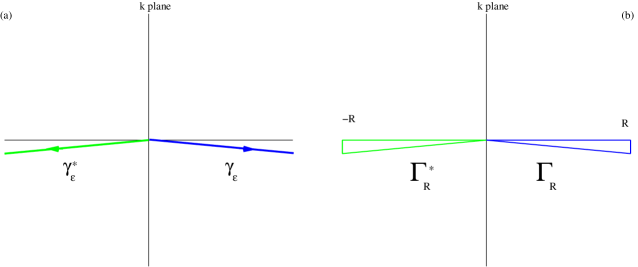
Figure 3: The contour $\gamma_{\varepsilon}$ is a radial path in the fourth quadrant that forms an angle $-\varepsilon$ with the positive $k$-axis. The contour $\Gamma_{R}$ consists of the segment $[0,R]$ of the positive real line, the arc $\gamma_{R}$, and the segment $\gamma_{\varepsilon,R}$ of length $R$ that forms an angle $-\varepsilon$ with the positive $k$-axis. The contours $\gamma_{\varepsilon}^{*}$ and $\Gamma_{R}^{*}$ are the mirror images of $\gamma_{\varepsilon}$ and $\Gamma_{R}$ with respect to the imaginary axis. If necessary, $\gamma_{\varepsilon}$ and $\gamma_{\varepsilon}^{*}$ may be bent to avoid resonances.

References

- [1] R. de la Madrid, J. Phys. A: Math. Gen. 39 (2006) (to be published).
- [2] H. M. Nussenzveig, Causality and Dispersion Relations, Academic Press, New York (1972).
- [3] M. Gadella, J. Math. Phys. 25, 2481 (1984).
- [4] A. Bohm, M. Gadella, “Dirac kets, Gamow vectors and Gelfand triplets,” Springer-Verlag, Berlin (1989).
- [5] M. Gadella, A. R. Ordonez, Int. J. Theor. Phys. 38, 131 (1999).
- [6] A. R. Bohm, R. de la Madrid, B. A. Tay, P. Kielanowski, hep-th/0101121.
- [7] A. R. Bohm, M. Loewe, B. Van de Ven, Fortschr. Phys. 51, 551 (2003); quant-ph/0212130.
- [8] M. Gadella, F. Gomez, J. Phys. A: Math. Gen. 35, 8505 (2002).
- [9] R. de la Madrid, Quantum Mechanics in rigged Hilbert space language, Ph.D. thesis, Universidad de Valladolid, Valladolid (2001). Available at http://www.physics.ucsd.edu/rafa/.
- [10] C. G. Bollini, O. Civitarese, A. L. De Paoli, M. C. Rocca, Phys. Lett. B382, 205 (1996).
- [11] C. G. Bollini, O. Civitarese, A. L. De Paoli, M. C. Rocca, J. Math. Phys. 37, 4235 (1996).
- [12] I. M. Gelfand, G. E. Shilov, Generalized Functions, Vol. III, Academic Press, New York (1967).
- [13] R. de la Madrid, Int. J. Theo. Phys. 42, 2441 (2003); quant-ph/0210167.
- [14] J. R. Taylor, Scattering theory, John Wiley & Sons, Inc., New York (1972).
- [15] R. Paley and N. Wiener, Fourier Transforms in the Complex Domain, American Mathematical Society, New York (1934).
- [16] E. Hille, Analytic Function Theory, Blaisdell, New York (1959).
- [17] P. Koosis, The Logarithmic Integral, Cambridge University Press, Cambridge, UK (1990).
- [18] A. Bohm, P. Kielanowski, S. Wickramasekara, “Complex energies and beginnings of time suggest a theory of scattering and decay,” quant-ph/0510060.
- [19] J. E. Roberts, J. Math. Phys. 7, 1097 (1966); Commun. Math. Phys. 3, 98 (1966).