The rigged Hilbert space approach to the Lippmann-Schwinger equation. Part I

Abstract

We exemplify the way the rigged Hilbert space deals with the Lippmann-Schwinger equation by way of the spherical shell potential. We explicitly construct the Lippmann-Schwinger bras and kets along with their energy representation, their time evolution and the rigged Hilbert spaces to which they belong. It will be concluded that the natural setting for the solutions of the Lippmann-Schwinger equation—and therefore for scattering theory—is the rigged Hilbert space rather than just the Hilbert space.

1 Introduction

Scattering experiments play a central role in our understanding of the microscopic world. For example, Compton scattering of x rays by electrons is held as experimental evidence for the particle nature of the photon; much of what has been learned about the structure of the nucleus, indeed even its discovery, was the results of scattering experiments; the analysis of scattering has yielded most of our present knowledge of elementary particle physics [1]. Scattering theory was developed in order to understand such experiments.

The Lippmann-Schwinger equation is one of the cornerstones of scattering theory. It was introduced by Lippmann and Schwinger in 1950 [2], and it has become a commonplace in scattering theory [3, 4, 5, 6]. It is written as

$$|E^{\pm}\rangle=|E\rangle+\frac{1}{E-H_{0}\pm\rmi\varepsilon}V|E^{\pm}\rangle\,,$$ (1.1)

where $|E^{\pm}\rangle$ represent the “in” and “out” Lippmann-Schwinger kets, $|E\rangle$ represents an eigenket of the free Hamiltonian $H_{0}$,

$$H_{0}|E\rangle=E|E\rangle\,,$$ (1.2)

and $V$ is the potential. The Lippmann-Schwinger kets are, in particular, eigenvectors of $H$:

$$H|E^{\pm}\rangle=E|E^{\pm}\rangle\,.$$ (1.3)

To the kets $|E^{\pm}\rangle$, there correspond the bras $\langle^{\pm}E|$, which satisfy

$$\langle^{\pm}E|=\langle E|+\langle^{\pm}E|V\frac{1}{E-H_{0}\mp\rmi\varepsilon}\,.$$ (1.4)

The bras $\langle^{\pm}E|$ are left eigenvectors of $H$,

$$\langle^{\pm}E|H=E\langle^{\pm}E|\,,$$ (1.5)

and the bras $\langle E|$ are left eigenvectors of $H_{0}$,

$$\langle E|H=E\langle E|\,.$$ (1.6)

In spite of its wide acceptance, the Lippmann-Schwinger equation still lacks a proper mathematical setting. There are mainly two problems. First, the bras $\langle^{\pm}E|$ and the kets $|E^{\pm}\rangle$ are not square integrable (i.e., they lie outside the Hilbert space), and therefore they must be treated as distributions. And second, in resonance theory the bras $\langle^{\pm}E|$ and the kets $|E^{\pm}\rangle$ need to be analytically continued into the complex plane [7, 8, 9, 10, 11, 12, 13, 14]. Both problems can be handled by means of the rigged Hilbert space (RHS). In this paper we shall focus on the first problem, namely on how to accommodate the Lippmann-Schwinger bras and kets for real, positive energies within the RHS setting. The second problem will be addressed in a sequel to this paper.

The present paper is the continuation of Refs. [15, 16, 17, 18], where we showed how the RHS deals with continuous spectrum. As we shall see, the methods of Refs. [15, 16, 17, 18] can be straightforwardly applied to the Lippmann-Schwinger equation.

We recall that a rigged Hilbert space is a triad of spaces (see Ref. [19] for a pedagogical introduction to the RHS)

$${\mathbf{\Phi}}\subset{\cal H}\subset{\mathbf{\Phi}}^{\times}$$ (1.7)

such that $\cal H$ is a Hilbert space, $\mathbf{\Phi}$ is a dense subspace of $\cal H$, and $\mathbf{\Phi}^{\times}$ is the space of antilinear functionals over $\mathbf{\Phi}$. The space $\mathbf{\Phi}^{\times}$ is called the antidual space of $\mathbf{\Phi}$. The space $\mathbf{\Phi}$ is the largest subspace of the Hilbert space such that first, it remains invariant under the action of the Hamiltonian, and second, the action of the Lippmann-Schwinger bras and kets is well defined on its elements. Associated with the RHS (1.7), there is always another RHS,

$${\mathbf{\Phi}}\subset{\cal H}\subset{\mathbf{\Phi}}^{\prime}\,,$$ (1.8)

where ${\mathbf{\Phi}}^{\prime}$ is called the dual space of ${\mathbf{\Phi}}$ and contains the linear functionals over $\mathbf{\Phi}$. As we shall show, the Lippmann-Schwinger bras $\langle^{\pm}E|$ belong to ${\mathbf{\Phi}}^{\prime}$, whereas the Lippmann-Schwinger kets $|E^{\pm}\rangle$ belong to ${\mathbf{\Phi}}^{\times}$.

It should be emphasized that our RHS does not entail an extension of the physical principles of scattering theory. Our RHS simply enables us to extract and process information contained in the Lippmann-Schwinger bras and kets.

There have been previous attempts at describing the Lippmann-Schwinger equation within the RHS setting in Refs. [8, 9, 10, 11, 12, 13, 14]. Our results will be different from those of [8, 9, 10, 11, 12, 13, 14] in the following sense. First, Refs. [8, 9, 10, 11, 12, 13, 14] use formal manipulations based on the Hardy-space assumption, whereas our approach is based on an explicitly solvable example; what is more, we do not make any assumption concerning Hardy functions, because Hardy functions seem unrelated to the solutions of the Lippmann-Schwinger equation. Second, Refs. [8, 9, 10, 11, 12, 13, 14] use two different RHSs (of Hardy functions), whereas we shall use only one RHS. Third, the Hardy-function assumption of Refs. [8, 9, 10, 11, 12, 13, 14] implies that the time evolution of the Lippmann-Schwinger bras and kets associated with real energies is given by a semigroup, whereas in this paper the time evolution of the Lippmann-Schwinger bras and kets is given by a group. And fourth, using Hardy functions as in Refs. [8, 9, 10, 11, 12, 13, 14] entails an extension of the physical principles of scattering theory, whereas in this paper we shall remain within standard quantum scattering theory.

The paper is organized as follows: In Sec. 2, we recall some of the basics of scattering theory. In Sec. 3, we obtain the Lippmann-Schwinger eigenfunctions in the radial, position representation for the spherical shell potential and for zero angular momentum. In Sec. 4, we recall the expressions for the domain, the spectrum and the Green function of the Hamiltonian. In Sec. 5, we obtain the unitary operators $U_{\pm}$, the eigenfunction expansions and the direct integral decompositions generated by the Lippmann-Schwinger eigenfunctions. In Sec. 6, we construct the Lippmann-Schwinger bras and kets from the corresponding eigenfunctions, and we obtain their most relevant properties. In Sec. 7, we calculate the time evolution of the Lippmann-Schwinger bras and kets. In Sec. 8, we justify some standard results of scattering theory within the RHS setting. In Sec. 9, we state our conclusions.

2 A reminder of scattering theory

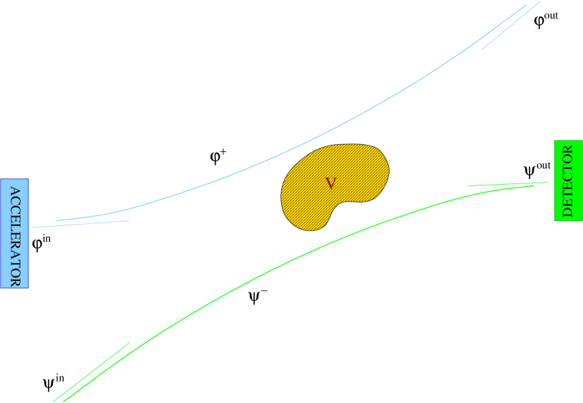
Figure 1: Schematic, pictorial representation of a scattering process.

A scattering process can be pictorially summarized as in Fig. 1. Loosely speaking, we send a beam of prepared initial “in” states $\varphi^{\rm in}$ toward the potential. After the collision takes place, $\varphi^{\rm in}$ becomes $\varphi^{\rm out}$. We then measure the probability to find a final “out” state $\psi^{\rm out}$. The amplitude of this probability is given by

$$(\psi^{\rm out},\varphi^{\rm out})=(\psi^{\rm out},S\varphi^{\rm in})\,,$$ (2.1)

where $S$ is the $S$ matrix. The state $\varphi^{\rm in}$ is determined by initial conditions through a preparation procedure (e.g., an accelerator). The state $\varphi^{\rm out}=S\varphi^{\rm in}$ is determined by those initial conditions through $\varphi^{\rm in}$ and by the scattering process through the $S$ matrix. The state $\psi^{\rm out}$ is determined by final conditions through a registration procedure (e.g., a detector).

The initial “in” state $\varphi^{\rm in}$ and the final “out” state $\psi^{\rm out}$ are asymptotic forms of the so-called “in” state $\varphi^{+}$ and “out” state $\psi^{-}$ in the remote past and in the distant future, respectively. In terms of these, the probability amplitude (2.1) reads

$$(\psi^{\rm out},\varphi^{\rm out})=(\psi^{-},\varphi^{+})\,.$$ (2.2)

The asymptotic states $\varphi^{\rm in}$ and $\psi^{\rm out}$ are related to the “exact” states $\varphi^{+}$ and $\psi^{-}$ by the Møller operators,

$$\Omega_{+}\varphi^{\rm in}=\varphi^{+}\,,$$ (2.3a)

$$\Omega_{-}\psi^{\rm out}=\psi^{-}\,.$$ (2.3b)

It is important to keep in mind that the states $\varphi^{\rm in}$, $\varphi^{\rm out}$ and $\psi^{\rm out}$ (or $\varphi^{+}$ and $\psi^{-}$) are not the central object of quantum scattering. The central object of quantum scattering is the probability amplitude (2.1)-(2.2), which measures the overlap between the “in” (i.e., prepared) and the “out” (i.e., detected) states. This is in distinction to classical scattering, where the states $\varphi^{\rm in}$, $\varphi^{+}$ and $\varphi^{\rm out}$ do actually represent a physical wave, and where we actually are able to observe $\varphi^{\rm out}$ rather than the overlap of $\varphi^{\rm out}$ with some $\psi^{\rm out}$.

It is customary to split up the (total) Hamiltonian $H$ into the free Hamiltonian $H_{0}$ and the potential $V$,

$$H=H_{0}+V\,.$$ (2.3d)

The potential $V$ is interpreted as the interaction between the components of the initial prepared states, for instance, the interaction between the in-going beam and the target. The states $\varphi^{\rm in}$ and $\psi^{\rm out}$ evolve under the influence of the free Hamiltonian $H_{0}$, whereas the states $\varphi^{+}$ and $\psi^{-}$ evolve under the influence of the (total) Hamiltonian $H$.

The dynamics of a scattering system is therefore governed by the Schrödinger equation subject to boundary conditions that specify what is “in” and what is “out.” The Lippmann-Schwinger equation (1.1) for the “in” $|E^{+}\rangle$ and “out” $|E^{-}\rangle$ kets has those “in” and “out” boundary conditions built into the $\pm\rmi\varepsilon$, since Eq. (1.1) is equivalent to the time-independent Schrödinger equation (1.3) subject to those “in” ($+\rmi\varepsilon$) and “out” ($-\rmi\varepsilon$) boundary conditions. In the position representation, the $+\rmi\varepsilon$ prescription yields the following asymptotic behavior:

$$\langle{\bf x}|E^{+}\rangle\,\smash{\mathop{\relbar\joinrel\longrightarrow}\limits_{r\to\infty}}\ \rme^{\rmi kz}+f(\theta,\phi)\,\frac{\rme^{\rmi kr}}{r}\,,$$ (2.3e)

where ${\bf x}\equiv(x,y,z)\equiv(r,\theta,\phi)$ are the position coordinates, $k$ is the wave number and $f(\theta,\phi)$ is the so-called scattering amplitude. Thus, far away from the potential region, $\langle{\bf x}|E^{+}\rangle$ is a linear combination of a plane wave (which originates from the free part in Eq. (1.1)) and an outgoing spherical wave multiplied by the scattering amplitude (which originate from the second term on the right-hand side of Eq. (1.1), and which account for the effect of the potential on the incoming beam). The $-\rmi\varepsilon$ prescription leads to the following asymptotic behavior:

$$\langle{\bf x}|E^{-}\rangle\,\smash{\mathop{\relbar\joinrel\longrightarrow}\limits_{r\to\infty}}\ \rme^{\rmi kz}+\overline{f(\theta,\phi)}\,\frac{\rme^{-\rmi kr}}{r}\,;$$ (2.3f)

thus, far away from the potential region, $\langle{\bf x}|E^{-}\rangle$ is a combination of a plane wave and an incoming spherical wave multiplied by the complex conjugate of $f(\theta,\phi)$.

Formally, the “in” state $\varphi^{+}$ and the “out” state $\psi^{-}$ can be expanded in terms of the Lippmann-Schwinger bras and kets as follows:

$$\varphi^{+}=\int_{0}^{\infty}\rmd E\,|E^{+}\rangle\langle^{+}\!\hskip 0.56917ptE|\varphi^{+}\rangle\,,$$ (2.3g)

$$\psi^{-}=\int_{0}^{\infty}\rmd E\,|E^{-}\rangle\langle^{-}E|\psi^{-}\rangle\,.$$ (2.3h)

The “in” (“out”) states can be also expanded in terms of the “out” (“in”) Lippmann-Schwinger bras and kets:

$$\varphi^{+}=\int_{0}^{\infty}\rmd E\,|E^{-}\rangle\langle^{-}E|\varphi^{+}\rangle\,,$$ (2.3i)

$$\psi^{-}=\int_{0}^{\infty}\rmd E\,|E^{+}\rangle\langle^{+}E|\psi^{-}\rangle\,.$$ (2.3j)

By combining Eqs. (2.3g)-(2.3h) with the relation

$$\langle^{-}E^{\prime}|E^{+}\rangle=S(E)\,\delta(E-E^{\prime})\,,$$ (2.3k)

we can express the matrix element (2.2) as

$$(\psi^{-},\varphi^{+})=\int_{0}^{\infty}\rmd E\,\langle\psi^{-}|E^{-}\rangle S(E)\langle^{+}\!\hskip 0.56917ptE|\varphi^{+}\rangle\,.$$ (2.3l)

Formally as well, the initial and final states can be expanded by the bras and kets of the free Hamiltonian:

$$\varphi^{\rm in}=\int_{0}^{\infty}\rmd E\,|E\rangle\langle E|\varphi^{\rm in}\rangle\,,$$ (2.3m)

$$\psi^{\rm out}=\int_{0}^{\infty}\rmd E\,|E\rangle\langle E|\psi^{\rm out}\rangle\,,$$ (2.3n)

and the probability amplitude (2.1) can be written as

$$(\psi^{\rm out},S\varphi^{\rm in})=\int_{0}^{\infty}\rmd E\,\langle\psi^{\rm out}|E\rangle S(E)\langle E|\varphi^{\rm in}\rangle\,,$$ (2.3o)

where we have used Eqs. (2.3m)-(2.3n) and the relation

$$\langle E^{\prime}|S|E\rangle=S(E)\,\delta(E-E^{\prime})\,.$$ (2.3p)

As we shall see in Sec. 8, the formal expressions (2.3g)-(2.3p) acquire meaning within the RHS.

3 Solving the Lippmann-Schwinger equation

For the spherical shell potential, the Lippmann-Schwinger equation can be solved explicitly. For the sake of focus, we shall restrict ourselves to angular momentum $l=0$.

3.1 The radial Lippmann-Schwinger equation

The expression for the spherical shell potential is given by

$$V({\bf x})\equiv V(r)=\left\{\begin{array}[]{ll}0&0<r<a\\ V_{0}&a<r<b\\ 0&b<r<\infty\,,\end{array}\right.$$ (2.3a)

where $V_{0}$ is a positive number that determines the strength of the potential, and $a$ and $b$ determine the positions in between which the potential is non-zero. Because the potential (2.3a) is spherically symmetric, we shall work in the radial position representation. In this representation and for $l=0$, the free Hamiltonian $H_{0}$ acts as the formal differential operator $h_{0}$,

$$H_{0}f(r)=h_{0}f(r)=-\frac{\hbar^{2}}{2m}\frac{\rmd^{2}}{\rmd r^{2}}f(r)\,,$$ (2.3b)

$V$ acts as multiplication by the rectangular barrier potential $V(r)$,

$$(Vf)(r)=V(r)f(r)\,,$$ (2.3c)

and the total Hamiltonian $H$ acts as the formal differential operator $h$,

$$Hf(r)=hf(r)=\left(-\frac{\hbar^{2}}{2m}\frac{\rmd^{2}}{\rmd r^{2}}+V(r)\right)f(r)\,.$$ (2.3d)

In the radial representation, the Lippmann-Schwinger equation (1.1) becomes

$$\langle r|E^{\pm}\rangle=\langle r|E\rangle+\langle r|\frac{1}{E-H_{0}\pm\rmi\varepsilon}V|E^{\pm}\rangle\,.$$ (2.3e)

In Eq. (2.3e), the $\langle r|E\rangle$ are eigenfunctions of the formal differential operator $h_{0}$,

$$h_{0}\langle r|E\rangle=E\langle r|E\rangle\,,$$ (2.3f)

whereas the $\langle r|E^{\pm}\rangle$ are eigenfunctions of the formal differential operator $h$,

$$h\langle r|E^{\pm}\rangle=E\langle r|E^{\pm}\rangle\,,$$ (2.3g)

subject to the boundary conditions specified by Eqs. (2.3ia)-(2.3ie).

3.2 The solutions to the radial Lippmann-Schwinger equation

The procedure to solve Eq. (2.3e) is well known [5, 6]. Since Eq. (2.3e) is an integral equation, it is equivalent to a differential equation subject to the boundary conditions that are built into that integral equation. In our case, for $l=0$, Eq. (2.3e) is equivalent to the Schrödinger differential equation,

$$\left(-\frac{\hbar^{2}}{2m}\frac{\rmd^{2}}{\rmd r^{2}}+V(r)\right)\langle r|E^{\pm}\rangle=E\langle r|E^{\pm}\rangle\,,$$ (2.3h)

subject to the following boundary conditions:

$$\langle r|E^{\pm}\rangle=0\,,$$ (2.3ia)

$$\langle r|E^{\pm}\rangle{\rm\ is\ continuous\ at\ }r=a,b\,,$$ (2.3ib)

$$\frac{\rmd}{\rmd r}\langle r|E^{\pm}\rangle{\rm\ is\ continuous\ at\ }r=a,b\,,$$ (2.3ic)

$$\langle r|E^{+}\rangle\sim\rme^{-\rmi kr}-S(E)\,\rme^{\rmi kr}\quad{\rm as\ }r\to\infty\,,$$ (2.3id)

$$\langle r|E^{-}\rangle\sim\rme^{\rmi kr}-\overline{S(E)}\,\rme^{-\rmi kr}\quad{\rm as\ }r\to\infty\,,$$ (2.3ie)

where

$$k=\sqrt{\frac{2m}{\hbar^{2}}E\,}$$ (2.3ij)

is the wave number, and $S(E)$ is the $S$ matrix in the energy representation. We recall that the boundary conditions (2.3id) and (2.3ie) originate from the $+\rmi\varepsilon$ and from the $-\rmi\varepsilon$ conditions of Eq. (2.3e), respectively. The boundary condition (2.3id) means that far away from the potential region, $\langle r|E^{+}\rangle$ is a combination of an incoming spherical wave and an outgoing spherical wave multiplied by the $S$ matrix. The boundary condition (2.3ie) means that far away from the potential region, $\langle r|E^{-}\rangle$ is a combination of an outgoing spherical wave and an incoming spherical wave multiplied by the complex conjugate of the $S$ matrix. The asymptotic behaviors (2.3id) and (2.3ie) are the $l=0$, radial counterparts of the asymptotic behaviors (2.3e) and (2.3f).

If we insert expression (2.3a) for the potential into Eq. (2.3h), and solve Eq. (2.3h) subject to the boundary conditions (2.3ia)-(2.3ie), we obtain the “in” and “out” eigenfunctions,

$$\langle r|E^{\pm}\rangle\equiv\chi^{\pm}(r;E)=N(E)\,\frac{\chi(r;E)}{{\cal J}_{\pm}(E)}\,,\qquad E\in[0,\infty)\,,$$ (2.3ik)

where $N(E)$ is a delta-normalization factor,

$$N(E)=\sqrt{\frac{1}{\pi}\frac{2m/\hbar^{2}}{\sqrt{2m/\hbar^{2}\,E\,}\,}\,}\,,$$ (2.3il)

$\chi(r;E)$ is the so-called regular solution of Eq. (2.3h),

$$\hskip-28.45274pt\chi(r;E)=\left\{\begin{array}[]{ll}\sin(\sqrt{\frac{2m}{\hbar^{2}}E\,}\,r)&0<r<a\\ {\cal J}_{1}(E)\rme^{\rmi\sqrt{\frac{2m}{\hbar^{2}}(E-V_{0})\,}\,r}+{\cal J}_{2}(E)\rme^{-\rmi\sqrt{\frac{2m}{\hbar^{2}}(E-V_{0})\,}\,r}&a<r<b\\ {\cal J}_{3}(E)\rme^{\rmi\sqrt{\frac{2m}{\hbar^{2}}E\,}\,r}+{\cal J}_{4}(E)\rme^{-\rmi\sqrt{\frac{2m}{\hbar^{2}}E\,}\,r}&b<r<\infty\,,\end{array}\right.$$ (2.3im)

and ${\cal J}_{\pm}(E)$ are the Jost functions,

$${\cal J}_{+}(E)=-2\rmi{\cal J}_{4}(E)\,,$$ (2.3ina)

$${\cal J}_{-}(E)=2\rmi{\cal J}_{3}(E)\,.$$ (2.3inb)

The explicit expressions for ${\cal J}_{1}$-${\cal J}_{4}$ can be obtained by matching the values of $\chi(r;E)$ and of its derivative at the discontinuities of the potential (see Eqs. (2.3insatalbcxagahaoa)-(2.3insatalbcxagahaod) in B). In terms of the Jost functions, the $S$ matrix is given by [5, 6]

$$S(E)=\frac{{\cal J}_{-}(E)}{{\cal J}_{+}(E)}\,,\qquad E\in[0,\infty)\,.$$ (2.3ino)

From Eq. (2.3ik) it follows that the “in” and “out” Lippmann-Schwinger eigenfunctions are proportional to each other,

$$\chi^{+}(r;E)=S(E)\,\chi^{-}(r;E)\,.$$ (2.3inp)

3.3 The “left” Lippmann-Schwinger eigenfunctions

When we write Eq. (1.4) in the radial position representation, we obtain an integral equation for the “left” Lippmann-Schwinger eigenfunctions,

$$\langle^{\pm}E|r\rangle=\langle E|r\rangle+\langle^{\pm}E|V\frac{1}{E-H_{0}\mp\rmi\varepsilon}|r\rangle\,.$$ (2.3inq)

Solving Eq. (2.3inq) is analogous to solving Eq. (2.3e). For $l=0$, Eq. (2.3inq) is equivalent to the Schrödinger differential equation,

$$\left(-\frac{\hbar^{2}}{2m}\frac{\rmd^{2}}{\rmd r^{2}}+V(r)\right)\langle^{\pm}E|r\rangle=E\langle^{\pm}E|r\rangle\,,$$ (2.3inr)

subject to the following boundary conditions:

$$\langle^{\pm}E|0\rangle=0\,,$$ (2.3insa)

$$\langle^{\pm}E|r\rangle{\rm\ is\ continuous\ at\ }r=a,b\,,$$ (2.3insb)

$$\frac{\rmd}{\rmd r}\langle^{\pm}E|r\rangle{\rm\ is\ continuous\ at\ }r=a,b\,,$$ (2.3insc)

$$\langle^{+}E|r\rangle\sim\rme^{\rmi kr}-\overline{S(E)}\,\rme^{-\rmi kr}\quad{\rm as\ }r\to\infty\,,$$ (2.3insd)

$$\langle^{-}E|r\rangle\sim\rme^{-\rmi kr}-S(E)\,\rme^{\rmi kr}\quad{\rm as\ }r\to\infty\,.$$ (2.3inse)

Note that the boundary conditions (2.3insd) and (2.3inse) originate from the $-\rmi\varepsilon$ and from the $+\rmi\varepsilon$ conditions of Eq. (2.3inq), respectively.

By inserting Eq. (2.3a) into Eq. (2.3inr), and by solving Eq. (2.3inr) subject to the boundary conditions (2.3insa)-(2.3inse), we obtain that the “left” Lippmann-Schwinger eigenfunctions $\langle^{\pm}E|r\rangle$ are the complex conjugates of the “right” Lippmann-Schwinger eigenfunctions $\langle r|E^{\pm}\rangle$,

$$\langle^{\pm}E|r\rangle\equiv\overline{\chi^{\pm}(r;E)}\,.$$ (2.3inst)

4 Domain, spectrum and resolvent

In this section, we include the expressions for the domain, the spectrum and the resolvent of $H$. Such expressions were obtained in Ref. [14], and are included in this section because we shall need them in subsequent sections.

The formal differential operator (2.3d) has an infinite number of self-adjoint extensions [20]. These self-adjoint extensions are characterized by the following boundary conditions [20]:

$$f(0)+\alpha\,f^{\prime}(0)=0\,,\quad-\infty<\alpha\leq\infty\,.$$ (2.3insa)

Among all these, the boundary condition needed in scattering theory is

$$f(0)=0\,.$$ (2.3insb)

The boundary condition (2.3insb) selects the following domain for the Hamiltonian:

$$\hskip-56.9055pt{\cal D}(H)=\left\{f(r)\,|\ f(r),hf(r)\in L^{2}([0,\infty),\rmd r),\,f(r)\in AC^{2}[0,\infty),\,f(0)=0\right\},$$ (2.3insc)

where $AC^{2}[0,\infty)$ denotes the space of functions whose first derivative is absolutely continuous. This domain induces a self-adjoint operator $H$,

$$(Hf)(r)=\left(-\frac{\hbar^{2}}{2m}\frac{\rmd^{2}}{\rmd r^{2}}+V(r)\right)f(r)\,,\quad f\in{\cal D}(H)\,.$$ (2.3insd)

The spectrum of $H$, ${\rm Sp}(H)$, was shown in Ref. [14] to be $[0,\infty)$. In Ref. [14], we also calculated the Green function $G(r,s;E)$ of $H$ for different regions of the complex energy plane. In all our calculations, we used the following branch for the square root function:

$$\hskip-56.9055pt\sqrt{\,\cdot\ }:\left\{E\in{\mathbb{C}}\,|\ -\pi<{\rm arg}(E)\leq\pi\right\}\longmapsto\left\{E\in{\mathbb{C}}\,|\ -\pi/2<{\rm arg}(E)\leq\pi/2\right\}\,.$$ (2.3inse)

The branch (2.3inse) grants the following relation:

$$\overline{\sqrt{\overline{E}\,}}=\sqrt{E}\,,\quad E\in\mathbb{C}\,,$$ (2.3insf)

which in general does not hold for other branches of the square root function.

Either by applying Theorem 1 of A, or by borrowing the results from Ref. [14], one can see that in the first quadrant of the energy plane, the Green function can be written as

$$\hskip-62.59596ptG(r,s;E)=\left\{\begin{array}[]{ll}-\pi N(E)\,\chi^{+}(r;E)\,f^{+}(s;E)&r<s\\[8.61108pt] -\pi N(E)\,\chi^{+}(s;E)\,f^{+}(r;E)&r>s\end{array}\right.\quad{\rm Re}(E)>0\,,\ {\rm Im}(E)>0\,,$$ (2.3insg)

whereas in the fourth quadrant its expression reads

$$\hskip-62.59596ptG(r,s;E)=\left\{\begin{array}[]{ll}-\pi N(E)\,\chi^{-}(r;E)\,f^{-}(s;E)&r<s\\[8.61108pt] -\pi N(E)\,\chi^{-}(s;E)\,f^{-}(r;E)&r>s\end{array}\right.\quad{\rm Re}(E)>0\,,\ {\rm Im}(E)<0\,.$$ (2.3insh)

In Eqs. (2.3insg)-(2.3insh), $\chi^{\pm}(r;E)$ are given by Eq. (2.3ik), $N(E)$ is given by Eq. (2.3il), and the eigenfunctions $f^{\pm}(r;E)$ are given by

$$\hskip-56.9055ptf^{\pm}(r;E)=\left\{\begin{array}[]{lll}{\cal A}^{\pm}_{1}(E)\rme^{\rmi\sqrt{\frac{2m}{\hbar^{2}}E\,}\,r}+{\cal A}^{\pm}_{2}(E)\rme^{-\rmi\sqrt{\frac{2m}{\hbar^{2}}E\,}\,r}&0<r<a\\ {\cal A}^{\pm}_{3}(E)\rme^{\rmi\sqrt{\frac{2m}{\hbar^{2}}(E-V_{0})\,}\,r}+{\cal A}^{\pm}_{4}(E)\rme^{-\rmi\sqrt{\frac{2m}{\hbar^{2}}(E-V_{0})\,}\,r}&a<r<b\\ \rme^{\pm\rmi\sqrt{\frac{2m}{\hbar^{2}}E\,}\,r}&b<r<\infty\,.\end{array}\right.$$ (2.3insi)

The coefficients ${\cal A}^{\pm}_{1}$-${\cal A}^{\pm}_{4}$ can be obtained by matching the values of $f^{\pm}(r;E)$ and of their derivatives at the discontinuities of the potential (see Eqs. (2.3insatalbcxagahaof)-(2.3insatalbcxagahaoi) in B).

5 The operators $U_{\pm}$ and $U_{0}$

In this section, we obtain the Fourier-like transforms $U_{\pm}$, the eigenfunction expansions and the direct integral decompositions generated by the “in” and “out” eigenfunctions. The operators $U_{\pm}$ will be obtained by applying the Sturm-Liouville theory (see Ref. [20] and A). We shall end this section by recalling the expression for the Fourier-like transform $U_{0}$ associated with the free Hamiltonian.

5.1 The “in” unitary operator $U_{+}$

The procedure to obtain $U_{+}$ consists of applying Theorems 2, 3 and 4 of A. In order to be able to apply Theorem 4, we choose the following basis for the space of solutions of $h\sigma=E\sigma$ that is continuous on $(0,\infty)\times(0,\infty)$ and analytically dependent on $E$ in a neighborhood of $(0,\infty)$:

$$\sigma_{1}(r;E)=\chi^{+}(r;E)\,,$$ (2.3insaa)

$$\sigma_{2}(r;E)=\left\{\begin{array}[]{lll}\cos(\sqrt{\frac{2m}{\hbar^{2}}E\,}\,r)&0<r<a\\ {\cal C}_{1}(E)\rme^{\rmi\sqrt{\frac{2m}{\hbar^{2}}(E-V_{0})\,}\,r}+{\cal C}_{2}(E)\rme^{-\rmi\sqrt{\frac{2m}{\hbar^{2}}(E-V_{0})\,}\,r}&a<r<b\\ {\cal C}_{3}(E)\rme^{\rmi\sqrt{\frac{2m}{\hbar^{2}}E\,}\,r}+{\cal C}_{4}(E)\rme^{-\rmi\sqrt{\frac{2m}{\hbar^{2}}E\,}\,r}&b<r<\infty\,.\end{array}\right.\quad$$ (2.3insae)

The functions ${\cal C}_{1}$-${\cal C}_{4}$ can be obtained by matching the values of $\sigma_{2}(r;E)$ and its first derivative at the discontinuities of the potential (see Eqs. (2.3insatalbcxagahaoj)-(2.3insatalbcxagahaom) in B). Equations (2.3insi) and (2.3insaa)-(2.3insae) lead to

$$f^{+}(r;E)=\frac{2\rmi{\cal J}_{4}(E){\cal C}_{4}(E)}{N(E)\,W(E)}\sigma_{1}(r;E)+\frac{{\cal J}_{4}(E)}{W(E)}\sigma_{2}(r;E)$$ (2.3insab)

and to

$$f^{-}(r;E)=-\frac{2\rmi{\cal J}_{4}(E){\cal C}_{3}(E)}{N(E)W(E)}\sigma_{1}(r;E)-\frac{{\cal J}_{3}(E)}{W(E)}\sigma_{2}(r;E)\,,$$ (2.3insac)

where

$$W(E)\equiv{\cal J}_{4}(E){\cal C}_{3}(E)-{\cal J}_{3}(E){\cal C}_{4}(E)\,.$$ (2.3insad)

After substituting Eq. (2.3insab) into Eq. (2.3insg) we arrive at

$$\hskip-28.45274pt\begin{array}[]{rl}G(r,s;E)=-\pi\,\frac{N(E)}{W(E)}\,\left[\frac{2\rmi{\cal J}_{4}(E){\cal C}_{4}(E)}{N(E)}\sigma_{1}(r;E)+{\cal J}_{4}(E)\sigma_{2}(r;E)\right]\sigma_{1}(s;E)\,,&\\[8.61108pt] \mbox{Re}(E)>0\,,\,\mbox{Im}(E)>0\,,\ r>s\,.&\end{array}$$ (2.3insae)

After substituting Eq. (2.3insac) into Eq. (2.3insh) we arrive at

$$\hskip-45.52458pt\begin{array}[]{rl}G(r,s;E)=-\pi\,\frac{N(E)}{W(E)}\frac{{\cal J}_{4}(E)}{{\cal J}_{3}(E)}\,\left[\frac{2\rmi{\cal J}_{4}(E){\cal C}_{3}(E)}{N(E)}\sigma_{1}(r;E)+{\cal J}_{3}(E)\sigma_{2}(r;E)\right]\sigma_{1}(s;E)\,,&\\[8.61108pt] \mbox{Re}(E)>0\,,\,\mbox{Im}(E)<0\,,\ r>s\,,&\end{array}$$ (2.3insaf)

where we have used the relation

$$\chi^{-}(r;E)=-\frac{{\cal J}_{4}(E)}{{\cal J}_{3}(E)}\chi^{+}(r;E)\,.$$ (2.3insag)

Because by Eq. (2.3insf)

$$\overline{\chi^{+}(s;\overline{E})}=-\frac{{\cal J}_{4}(E)}{{\cal J}_{3}(E)}\chi^{+}(s;E)\,,$$ (2.3insah)

Eq. (2.3insae) leads to

$$\hskip-48.36958pt\begin{array}[]{rl}G(r,s;E)=2\pi\rmi\frac{{\cal J}_{3}(E){\cal C}_{4}(E)}{W(E)}\,\sigma_{1}(r;E)\overline{\sigma_{1}(s;\overline{E})}+\pi\frac{N(E){\cal J}_{3}(E)}{W(E)}\,\sigma_{2}(r;E)\overline{\sigma_{1}(s;\overline{E})}\,,&\\[8.61108pt] \mbox{Re}(E)>0\,,\,\mbox{Im}(E)>0\,,\ r>s\,,&\end{array}$$ (2.3insai)

and Eq. (2.3insaf) leads to

$$\hskip-48.36958pt\begin{array}[]{rl}G(r,s;E)=2\pi\rmi\frac{{\cal J}_{4}(E){\cal C}_{3}(E)}{W(E)}\,\sigma_{1}(r;E)\overline{\sigma_{1}(s;\overline{E})}+\pi\frac{N(E){\cal J}_{3}(E)}{W(E)}\,\sigma_{2}(r;E)\overline{\sigma_{1}(s;\overline{E})}\,,&\\[8.61108pt] \mbox{Re}(E)>0\,,\,\mbox{Im}(E)<0\,,\ r>s\,.&\end{array}$$ (2.3insaj)

On the other hand, the Green function can be written in terms of the basis $\left\{\sigma_{1},\sigma_{2}\right\}$ of Eqs. (2.3insaa)-(2.3insae) as (see Eq. (2.3insatalbcxagahaoi) in Theorem 4)

$$G(r,s;E)=\sum_{i,j=1}^{2}\theta_{ij}^{+}(E)\sigma_{i}(r;E)\overline{\sigma_{j}(s;\overline{E})}\,,\qquad r>s\,.$$ (2.3insak)

By comparing (2.3insak) to (2.3insai), we obtain

$$\theta_{ij}^{+}(E)=\left(\begin{array}[]{cc}2\pi\rmi\frac{{\cal J}_{3}(E){\cal C}_{4}(E)}{W(E)}&0\\ \pi\frac{N(E){\cal J}_{3}(E)}{W(E)}&0\end{array}\right),\quad\mbox{Re}(E)>0\,,\ \mbox{Im}(E)>0\,.$$ (2.3insal)

By comparing (2.3insak) to (2.3insaj), we obtain

$$\theta_{ij}^{+}(E)=\left(\begin{array}[]{cc}2\pi\rmi\frac{{\cal J}_{4}(E){\cal C}_{3}(E)}{W(E)}&0\\ \pi\frac{N(E){\cal J}_{3}(E)}{W(E)}&0\end{array}\right),\quad\mbox{Re}(E)>0\,,\ \mbox{Im}(E)<0\,.$$ (2.3insam)

From Eqs. (2.3insal) and (2.3insam) it follows that the measures $\rho_{12}$, $\rho_{21}$ and $\rho_{22}$ of Eq. (2.3insatalbcxagahaoj) are zero, and that $\rho_{11}$ is given by

$$\rho_{11}((E_{1},E_{2})) = \frac{1}{2\pi\rmi}\int_{E_{1}}^{E_{2}}2\pi\rmi\frac{{\cal J}_{4}(E){\cal C}_{3}(E)-{\cal J}_{3}(E){\cal C}_{4}(E)}{W(E)}\rmd E$$ (2.3insan)

$$= \int_{E_{1}}^{E_{2}}\rmd E=E_{2}-E_{1}\,,$$

where we have used (2.3insad) in the second step. Therefore, the measure $\rho_{11}$ is just the Lebesgue measure, which means, in particular, that the eigenfunctions $\chi^{+}(r;E)$ are $\delta$-normalized (see also Sec. 2.9 of Ref. [16]).

By Theorem 2 of A, there is a unitary operator $U_{+}$ that transforms from the position representation into the energy representation,

$$\hskip-28.45274pt\begin{array}[]{rcl}U_{+}:L^{2}([0,\infty),\rmd r)&\longmapsto&L^{2}([0,\infty),\rmd E)\\[4.30554pt] f(r)&\longmapsto&\widehat{f}_{+}(E)=(U_{+}f)(E)=\int_{0}^{\infty}\rmd rf(r)\overline{\chi^{+}(r;E)}\,,\end{array}$$ (2.3insao)

where $\widehat{f}_{+}(E)$ denotes the energy representation of the function $f(r)$ when obtained by way of $U_{+}$. The action of $U_{+}$ on the domain ${\cal D}(H)$ is given by

$$\hskip-42.67912pt{\cal D}(\widehat{H})=U_{+}{\cal D}(H)=\left\{\widehat{f}_{+}(E)\in L^{2}([0,\infty),\rmd E)\,|\ \int_{0}^{\infty}\rmd E\,|E\widehat{f}_{+}(E)|^{2}<\infty\right\}.$$ (2.3insap)

It can be easily checked that the operator $U_{+}$ diagonalizes $H$ in the sense that $\widehat{H}\equiv U_{+}HU_{+}^{-1}$ acts as the operator multiplication by $E$,

$$\begin{array}[]{rcl}\widehat{H}:{\cal D}(\widehat{H})\subset L^{2}([0,\infty),\rmd E)&\longmapsto&L^{2}([0,\infty),\rmd E)\\[4.30554pt] \widehat{f}_{+}&\longmapsto&\widehat{H}\widehat{f}_{+}(E)=E\widehat{f}_{+}(E)\,.\end{array}$$ (2.3insaq)

The inverse of $U_{+}$ is given by Eq. (2.3insatalbcxagahaof):

$$\hskip-42.67912ptf(r)=U_{+}^{-1}\widehat{f}_{+}(r)=\int_{0}^{\infty}\rmd E\,\widehat{f}_{+}(E)\chi^{+}(r;E)\,,\quad\widehat{f}_{+}(E)\in L^{2}([0,\infty),\rmd E)\,.$$ (2.3insar)

The operator $U_{+}^{-1}$ transforms from the energy representation back into the position representation. Expressions (2.3insao) and (2.3insar) provide the eigenfunction expansions of any square integrable function in terms of the “in” eigensolutions.

The operator $U_{+}$, and therefore the “in” eigenfunctions $\chi^{+}(r;E)$, entails a direct integral decomposition of the Hilbert space in a straightforward manner:

$$\begin{array}[]{rcl}{\cal H}&\longmapsto&U_{+}{\cal H}\equiv\widehat{\cal H}=\oplus\int_{{\rm Sp}(H)}{\cal H}(E)\rmd E\\[4.30554pt] f&\longmapsto&U_{+}f\equiv\left\{\widehat{f}_{+}(E)\right\},\,\quad f\in{\cal D}(H)\,,\,\widehat{f}_{+}(E)\in{\cal H}(E)\,.\end{array}$$ (2.3insas)

In this equation, the Hilbert spaces ${\cal H}$, $\widehat{\cal H}$ and ${\cal H}(E)$ are respectively realized by $L^{2}([0,\infty),\rmd r)$, $L^{2}([0,\infty),\rmd E)$ and $\mathbb{C}$.

5.2 The “out” unitary operator $U_{-}$

The construction of $U_{-}$ follows the same procedure as the construction of $U_{+}$. The functions

$$\sigma_{1}(r;E)=\chi^{-}(r;E)\,,$$ (2.3insata)

$$\sigma_{2}(r;E)=\left\{\begin{array}[]{lll}\cos(\sqrt{\frac{2m}{\hbar^{2}}E\,}\,r)&0<r<a\\ {\cal C}_{1}(E)\rme^{\rmi\sqrt{\frac{2m}{\hbar^{2}}(E-V_{0})\,}\,r}+{\cal C}_{2}(E)\rme^{-\rmi\sqrt{\frac{2m}{\hbar^{2}}(E-V_{0})\,}\,r}&a<r<b\\ {\cal C}_{3}(E)\rme^{\rmi\sqrt{\frac{2m}{\hbar^{2}}E\,}\,r}+{\cal C}_{4}(E)\rme^{-\rmi\sqrt{\frac{2m}{\hbar^{2}}E\,}\,r}&b<r<\infty\end{array}\right.\quad$$ (2.3insate)

form another basis for the space of solutions of $h\sigma=E\sigma$ that is continuous on $(0,\infty)\times(0,\infty)$ and analytically dependent on $E$ in a neighborhood of $(0,\infty)$. Therefore, we are allowed to apply Theorem 4 of A. Equations (2.3insi) and (2.3insata)-(2.3insate) lead to

$$f^{+}(r;E)=-\frac{2\rmi{\cal J}_{3}(E){\cal C}_{4}(E)}{N(E)W(E)}\sigma_{1}(r;E)+\frac{{\cal J}_{4}(E)}{W(E)}\sigma_{2}(r;E)$$ (2.3insatu)

and to

$$f^{-}(r;E)=\frac{2\rmi{\cal J}_{3}(E){\cal C}_{3}(E)}{N(E)W(E)}\sigma_{1}(r;E)-\frac{{\cal J}_{3}(E)}{W(E)}\sigma_{2}(r;E)\,.$$ (2.3insatv)

By substituting Eqs. (2.3insatu) and (2.3insag) into Eq. (2.3insg), we obtain

$$\hskip-56.9055pt\begin{array}[]{rl}G(r,s;E)=\pi\,N(E)\,\frac{{\cal J}_{3}(E)}{{\cal J}_{4}(E)}\left[-\frac{2\rmi{\cal J}_{3}(E){\cal C}_{4}(E)}{N(E)W(E)}\sigma_{1}(r;E)+\frac{{\cal J}_{4}(E)}{W(E)}\sigma_{2}(r;E)\right]\sigma_{1}(s;E)\,,&\\[4.30554pt] \mbox{Re}(E)>0\,,\,\mbox{Im}(E)>0\,,\ r>s\,.&\end{array}$$ (2.3insatw)

By substituting Eq. (2.3insatv) into Eq. (2.3insh), we obtain

$$\hskip-42.67912pt\begin{array}[]{rl}G(r,s;E)=-\pi\,N(E)\,\left[\frac{2\rmi{\cal J}_{3}(E){\cal C}_{3}(E)}{N(E)W(E)}\sigma_{1}(r;E)-\frac{{\cal J}_{3}(E)}{W(E)}\sigma_{2}(r;E)\right]\sigma_{1}(s;E)\,,&\\[4.30554pt] \mbox{Re}(E)>0\,,\,\mbox{Im}(E)<0\,,\ r>s\,.&\end{array}$$ (2.3insatx)

Because by Eq. (2.3insf)

$$\overline{\chi^{-}(s;\overline{E})}=-\frac{{\cal J}_{3}(E)}{{\cal J}_{4}(E)}\chi^{-}(s;E)\,,$$ (2.3insaty)

Eq. (2.3insatw) leads to

$$\hskip-42.67912pt\begin{array}[]{rl}G(r,s;E)=2\pi\rmi\frac{{\cal J}_{3}(E){\cal C}_{4}(E)}{W(E)}\sigma_{1}(r;E)\overline{\sigma_{1}(s;\overline{E})}-\pi\frac{N(E){\cal J}_{4}(E)}{W(E)}\sigma_{2}(r;E)\overline{\sigma_{1}(s;\overline{E})}\,,&\\[4.30554pt] \mbox{Re}(E)>0\,,\,\mbox{Im}(E)>0\,,\ r>s\,,&\end{array}$$ (2.3insatz)

and Eq. (2.3insatx) leads to

$$\hskip-42.67912pt\begin{array}[]{rl}G(r,s;E)=2\pi\rmi\frac{{\cal J}_{4}(E){\cal C}_{3}(E)}{W(E)}\sigma_{1}(r;E)\overline{\sigma_{1}(s;\overline{E})}-\pi\frac{N(E){\cal J}_{4}(E)}{W(E)}\sigma_{2}(r;E)\overline{\sigma_{1}(s;\overline{E})}\,,&\\[4.30554pt] \mbox{Re}(E)>0\,,\,\mbox{Im}(E)<0\,,\ r>s\,.\end{array}$$ (2.3insataa)

On the other hand, by way of Eq. (2.3insatalbcxagahaoi), we can write the Green function in terms of the basis $\left\{\sigma_{1},\sigma_{2}\right\}$ of Eqs. (2.3insata)-(2.3insate) as

$$G(r,s;E)=\sum_{i,j=1}^{2}\theta_{ij}^{+}(E)\sigma_{i}(r;E)\overline{\sigma_{j}(s;\overline{E})}\,,\qquad r>s\,.$$ (2.3insatab)

By comparing (2.3insatab) to (2.3insatz), we obtain

$$\theta_{ij}^{+}(E)=\left(\begin{array}[]{cc}2\pi\rmi\frac{{\cal J}_{3}(E){\cal C}_{4}(E)}{W(E)}&0\\ -\pi\frac{N(E){\cal J}_{4}(E)}{W(E)}&0\end{array}\right),\quad\mbox{Re}(E)>0\,,\ \mbox{Im}(E)>0\,.$$ (2.3insatac)

By comparing (2.3insatab) to (2.3insataa), we obtain

$$\theta_{ij}^{+}(E)=\left(\begin{array}[]{cc}2\pi\rmi\frac{{\cal J}_{4}(E){\cal C}_{3}(E)}{W(E)}&0\\ -\pi\frac{N(E){\cal J}_{4}(E)}{W(E)}&0\end{array}\right),\quad\mbox{Re}(E)>0\,,\ \mbox{Im}(E)<0\,.$$ (2.3insatad)

From Eqs. (2.3insatac), (2.3insatad) and (2.3insatalbcxagahaoj), it follows that the measures $\rho_{12}$, $\rho_{21}$ and $\rho_{22}$ in Theorem 4 of A are zero, and that $\rho_{11}$ is given by the Lebesgue measure,

$$\rho_{11}((E_{1},E_{2}))=\int_{E_{1}}^{E_{2}}\rmd E=E_{2}-E_{1}\,.$$ (2.3insatae)

This means, in particular, that the $\chi^{-}(r;E)$ are $\delta$-normalized.

By Theorem 2 of A, there is a unitary operator $U_{-}$ that transforms from the position into the energy representation,

$$\hskip-14.22636pt\widehat{f}_{-}(E)=(U_{-}f)(E)=\int_{0}^{\infty}\rmd rf(r)\overline{\chi^{-}(r;E)}\,,\quad f(r)\in L^{2}([0,\infty),\rmd r)\,,$$ (2.3insataf)

where $\widehat{f}_{-}(E)$ denotes the energy representation of $f(r)$ when obtained by way of $U_{-}$. The inverse of $U_{-}$ is given by Eq. (2.3insatalbcxagahaof):

$$\hskip-36.98866ptf(r)=(U_{-}^{-1}\widehat{f}_{-})(r)=\int_{0}^{\infty}\rmd E\,\widehat{f}_{-}(E)\chi^{-}(r;E)\,,\quad\widehat{f}_{-}(E)\in L^{2}([0,\infty),\rmd E)\,.$$ (2.3insatag)

Likewise $U_{+}^{-1}$, the operator $U_{-}^{-1}$ transforms from the energy representation into the position representation. Likewise $U_{+}$, $U_{-}$ carries the domain ${\cal D}(H)$ onto the domain (2.3insap), and $\widehat{H}\equiv U_{-}HU_{-}^{-1}$ acts as the operator multiplication by $E$. As well, expressions (2.3insataf) and (2.3insatag) provide the expansions of any square integrable function in terms of the “out” eigenfunctions, and a direct integral decomposition similar to (2.3insas).

5.3 The “free” unitary operator $U_{0}$

The operator $U_{0}$ was constructed in Refs. [14, 17]. Because we shall need $U_{0}$ in order to construct the Møller operators, in this subsection we recall the expression for $U_{0}$.

The regular (i.e., vanishing at $r=0$), $\delta$-normalized eigensolution of the differential operator (2.3b) is given by

$$\chi_{0}(r;E)=N(E)\sin\left(\sqrt{\frac{2m}{\hbar^{2}}E\,}\,r\right),\quad 0<r<\infty\,.$$ (2.3insatah)

This eigensolution can be used to construct the unitary operator

$$\begin{array}[]{rcl}U_{0}:L^{2}([0,\infty),\rmd r)&\longmapsto&L^{2}([0,\infty),\rmd E)\\[4.30554pt] f&\longmapsto&U_{0}f\equiv{\widehat{f}}_{0}\end{array}$$ (2.3insatai)

that transforms from the position into the energy representation. The action of $U_{0}$ can be written as an integral operator:

$$\widehat{f}_{0}(E)=U_{0}f(E)=\int_{0}^{\infty}\rmd rf(r)\overline{\chi_{0}(r;E)}\,,\quad f(r)\in L^{2}([0,\infty),\rmd r)\,,$$ (2.3insataj)

where $\widehat{f}_{0}(E)$ denotes the energy representation of $f(r)$ when obtained by way of $U_{0}$. The inverse of $U_{0}$ can also be written as an integral operator:

$$\hskip-28.45274ptf(r)=U_{0}^{-1}\widehat{f}_{0}(r)=\int_{0}^{\infty}\rmd E\,\widehat{f}_{0}(E)\chi_{0}(r;E)\,,\quad\widehat{f}_{0}(E)\in L^{2}([0,\infty),\rmd E)\,.$$ (2.3insatak)

Expressions (2.3insataj) and (2.3insatak) provide the expansions of any square integrable function in terms of the “free” eigenfunctions.

Note that, since the Lippmann-Schwinger eigenfunctions tend to the “free” eigenfunctions when the potential vanishes,

$$\lim_{V_{0}\to 0}\chi^{\pm}(r;E)=\chi_{0}(r;E)\,,$$ (2.3insatala)

the operators $$U_{\pm} U_{0}$$ tend to when the potential vanishes,

$$\lim_{V_{0}\to 0}U_{\pm}=U_{0}\,.$$ (2.3insatalb)

6 Construction of the “in” and “out” bras and kets

The solutions to the Lippmann-Schwinger equation are eigenvectors of the Hamiltonian whose eigenvalues lie in the continuous spectrum. As explained throughly in Refs. [14, 19], eigenvectors whose eigenvalues lie in the continuous spectrum must be treated as distributions by way of the rigged Hilbert space. In this section, we construct the “in” and “out” bras and kets together with the rigged Hilbert spaces that accommodate them. As it turns out, the RHS constructed in Refs. [14, 15, 16] suffices for such purpose. The results of this section will be summarized by Proposition 1 at the end of this section.

6.1 The “in” kets

The definition of a ket is borrowed from the theory of distributions [21]. Given a function $f(x)$ and a space of test functions $\mathbf{\Phi}$, the antilinear functional $F$ associated with the function $f(x)$ is an integral operator whose kernel is precisely $f(x)$:

$$F(\varphi)=\int\rmd x\,\overline{\varphi(x)}f(x)\,.$$ (2.3insatala)

The “bad behavior” of the distribution $f(x)$ must be compensated by the “nice behavior” of the test function $\varphi(x)$, so the integral (2.3insatala) makes sense.

By using definition (2.3insatala), we associate an “in” ket $|E^{+}\rangle$ with the “in” eigenfunction $\chi^{+}(r;E)$ for each $E\in[0,\infty)$:

$$\begin{array}[]{rcl}|E^{+}\rangle:{\mathbf{\Phi}}&\longmapsto&{\mathbb{C}}\\ \varphi^{+}&\longmapsto&\langle\varphi^{+}|E^{+}\rangle\equiv\int_{0}^{\infty}\rmd r\,\overline{\varphi^{+}(r)}\chi^{+}(r;E)\,.\end{array}$$ (2.3insatalba)

In Dirac’s notation, the action of $$|E^{+}\rangle$$ is written as

$$\langle\varphi^{+}|E^{+}\rangle\equiv\int_{0}^{\infty}\rmd r\,\langle\varphi^{+}|r\rangle\langle r|E^{+}\rangle\,.$$ (2.3insatalbb)

Note that even though $\chi^{+}(r;E)\equiv\langle r|E^{+}\rangle$ is also meaningful for complex energies, the energy in Eqs. (2.3insatalba)-(2.3insatalbb) runs only over ${\rm Sp}(H)=[0,\infty)$, because in this paper we restrict ourselves to bras and kets associated with energies that belong to the spectrum of the Hamiltonian.

We now need to find the subspace $\mathbf{\Phi}$ on which definition (2.3insatalba) makes sense. Besides making (2.3insatalba) well defined, the space ${\mathbf{\Phi}}$ must also be invariant under the action of the observables of the system. The invariance of $\mathbf{\Phi}$ is a crucial property, since it entails finite expectation values and well-defined commutation relations, and since it allows us to apply observables on the elements of $\mathbf{\Phi}$ as many times as wished [19]. Since in this paper the only observable we are concerned with is the Hamiltonian, we shall simply require invariance under $H$. Thus, the space $\mathbf{\Phi}$ must satisfy the following conditions:

$$\bullet\ \,{\rm The\ space\ }{\mathbf{\Phi}}\ {\rm is\ invariant\ under\ the\ action\ of}\ H.$$ (2.3insatalbca)

$$\bullet\ \,{\rm The\ elements\ of\ }{\mathbf{\Phi}}\ {\rm are\ such\ that\ the\ integral\ in\ Eq.~{}(\ref{LSdefinitionket+E})\ makes\ sense.}$$ (2.3insatalbcb)

In order to meet requirement (2.3insatalbca), the wave functions $\varphi^{+}(r)$ must at least be in the maximal invariant subspace of $H$:

$${\cal D}=\bigcap_{n=0}^{\infty}{\cal D}(H^{n})\,.$$ (2.3insatalbcd)

As shown in Refs. [14, 16], the space ${\cal D}$ is given by

$$\begin{array}[]{ll}\hskip-56.9055pt{\cal D}=\left\{\varphi\in L^{2}([0,\infty),\rmd r)\,|\ \right.&h^{n}\varphi(r)\in L^{2}([0,\infty),\rmd r),\ \varphi^{(n)}(a)=\varphi^{(n)}(b)=0,\\ \hskip-56.9055pt&\left.h^{n}\varphi(0)=0,n=0,1,2,\ldots;\ \varphi(r)\in C^{\infty}([0,\infty))\right\},\end{array}$$ (2.3insatalbce)

where $\varphi^{(n)}$ denotes the $n$th derivative of $\varphi$. In order to meet requirement (2.3insatalbcb), the wave functions $\varphi^{+}(r)$ must behave well enough so the integral in Eq. (2.3insatalba) is well defined and yields a continuous, antilinear functional. From the expression for $\chi^{+}(r;E)$, Eq. (2.3ik), one can see that the $\varphi^{+}(r)$ have essentially to control purely imaginary exponentials. Therefore, the space $\mathbf{\Phi}$ constructed in Refs. [14, 16] meets the requirements (2.3insatalbca)-(2.3insatalbcb):

$$\hskip-36.98866pt{\mathbf{\Phi}}=\left\{\varphi^{+}\in L^{2}([0,\infty),\rmd r)\,|\ \varphi^{+}\in{\cal D}\,,\ \|\varphi^{+}\|_{n,m}<\infty\,,\ n,m=0,1,2,\ldots\right\},$$ (2.3insatalbcf)

where the $\|\ \|_{n,m}$ are given by

$$\hskip-42.67912pt\|\varphi^{+}\|_{n,m}:=\sqrt{\int_{0}^{\infty}\rmd r\,\left|(1+r)^{n}(1+H)^{m}\varphi^{+}(r)\right|^{2}\,}\,,\quad n,m=0,1,2,\ldots\,.$$ (2.3insatalbcg)

The space $\mathbf{\Phi}$ is the collection of square integrable functions that belong to the maximal invariant subspace of $H$ and for which the estimates (2.3insatalbcg) are finite. In particular, because $\varphi^{+}(r)$ satisfies the estimates (2.3insatalbcg), $\varphi^{+}(r)$ falls off at infinity faster than any polynomial of $r$:

$$\lim_{r\to\infty}(1+r)^{n}\varphi^{+}(r)=0\,,\quad n=0,1,2,\ldots\,.$$ (2.3insatalbch)

Obviously, the space ${\mathbf{\Phi}}$ can also be seen as the maximal invariant subspace of the algebra generated by the Hamiltonian and the operator multiplication by $r$. The estimates (2.3insatalbcg) are norms (see Proposition 1 at the end of this section), and therefore they define a topology (i.e., a meaning of convergence of sequences) $\tau_{\mathbf{\Phi}}$ on $\mathbf{\Phi}$:

$$\varphi^{+}_{\alpha}\,\smash{\mathop{\relbar\joinrel\longrightarrow}\limits^{\tau_{\mathbf{\Phi}}}_{\alpha\to\infty}}\,\varphi^{+}\quad{\rm iff}\quad\|\varphi^{+}_{\alpha}-\varphi^{+}\|_{n,m}\,\smash{\mathop{\relbar\joinrel\longrightarrow}\limits_{\alpha\to\infty}}\,0\,,\quad n,m=0,1,2,\ldots\,.$$ (2.3insatalbci)

Once we have constructed the space $\mathbf{\Phi}$, we can construct its topological dual $\mathbf{\Phi}^{\times}$ as the space of ${\mathbf{\Phi}}$-continuous antilinear functionals on $\mathbf{\Phi}$, and therewith the RHS corresponding to the “in” states,

$${\mathbf{\Phi}}\subset L^{2}([0,\infty),\rmd r)\subset{\mathbf{\Phi}}^{\times}\,.$$ (2.3insatalbcj)

One can show that $|E^{+}\rangle$ indeed belongs to ${\mathbf{\Phi}}^{\times}$, see Proposition 1 below.

The conditions (2.3insatalbce) and (2.3insatalbcg) that determine the space $\mathbf{\Phi}$ are very similar to the conditions satisfied by the Schwartz space on the positive real line, the major difference being that the derivatives of the elements of $\mathbf{\Phi}$ vanish at $r=0,a,b$. This is why we shall write

$${\mathbf{\Phi}}\equiv{\cal S}(\mathbb{R}^{+}\!\frac{\ }{\ }\{a,b\})\,,$$ (2.3insatalbck)

where ${\mathbb{R}}^{+}\equiv[0,\infty)$. With this notation, the RHS (2.3insatalbcj) can be written as

$${\cal S}(\mathbb{R}^{+}\!\frac{\ }{\ }\{a,b\})\subset L^{2}(\mathbb{R}^{+},\rmd r)\subset{\cal S}^{\times}(\mathbb{R}^{+}\!\frac{\ }{\ }\{a,b\})\,.$$ (2.3insatalbcl)

The “in” kets should be eigenvectors of $H$ as in Eq. (1.3). However, since the Hamiltonian acts in principle only on its Hilbert space domain, and since the “in” kets belong to the antidual rather than to the Hilbert space, we need to extend the action of $H$ from $\mathbf{\Phi}$ to $\mathbf{\Phi}^{\times}$, in order to specify how $H$ acts on $|E^{+}\rangle$. The theory of distributions provides us with a precise prescription for such extension: Given an operator $A$, the action of $A$ on a functional $|F\rangle\in{\mathbf{\Phi}}^{\times}$ is defined as

$$\langle\varphi|A|F\rangle\equiv\langle A^{\dagger}\varphi|F\rangle\,,\quad\mbox{for all}\ \varphi\ \mbox{in}\ \mathbf{\Phi}\,.$$ (2.3insatalbcm)

It is important to realize that definition (2.3insatalbcm) makes sense only when $\mathbf{\Phi}$ is invariant under $A^{\dagger}$,

$$A^{\dagger}{\mathbf{\Phi}}\subset{\mathbf{\Phi}}\,.$$ (2.3insatalbcn)

Note that when $A$ is self-adjoint (e.g., $A=H$), then $A^{\dagger}=A$, and when $A$ is unitary (e.g., $A=U_{+}$), then $A^{\dagger}=A^{-1}$. Definition (2.3insatalbcm) can in turn be used to define the notion of eigenket of a self-adjoint observable: A functional $|a\rangle$ in $\mathbf{\Phi}^{\times}$ is an eigenket of $A$ with eigenvalue $a$ if

$$\langle\varphi|A|a\rangle=\langle A\varphi|a\rangle=a\langle\varphi|a\rangle\,,\quad\mbox{for all}\ \varphi\ \mbox{in}\ \mathbf{\Phi}\,.$$ (2.3insatalbco)

When the “left sandwiching” of this equation with the elements of $\mathbf{\Phi}$ is understood and therefore omitted, we shall simply write

$$A|a\rangle=a|a\rangle\,.$$ (2.3insatalbcp)

Thus, within the RHS setting, the eigenvalue equation (1.3) is to be understood as

$$\langle\varphi^{+}|H|E^{+}\rangle=E\langle\varphi^{+}|E^{+}\rangle\,,\quad\varphi^{+}\in{\mathbf{\Phi}}\,.$$ (2.3insatalbcq)

This eigenvalue equation is proved in Proposition 1.

By means of the unitary operator $U_{+}$, which was constructed in Section 5.1, we can obtain the energy representation of the space ${\mathbf{\Phi}}$,

$$U_{+}{\mathbf{\Phi}}=\widehat{\mathbf{\Phi}}_{+}\,.$$ (2.3insatalbcr)

We shall denote the elements of $\widehat{\mathbf{\Phi}}_{+}$ by $\widehat{\varphi}^{+}(E)\equiv(U_{+}\varphi^{+})(E)$, where $E\in[0,\infty)$. Using the notation of Eq. (2.3insatalbck), the space $\widehat{\mathbf{\Phi}}_{+}$ will be also denoted as

$$\widehat{\mathbf{\Phi}}_{+}\equiv\widehat{{\cal S}}_{+}(\mathbb{R}^{+}\!\frac{\ }{\ }\{a,b\})\,,$$ (2.3insatalbcs)

and the energy representations of the triplets (2.3insatalbcj) and (2.3insatalbcl) will be respectively denoted by

$$\widehat{\mathbf{\Phi}}_{+}\subset L^{2}([0,\infty),\rmd E)\subset\widehat{\mathbf{\Phi}}_{+}^{\times}$$ (2.3insatalbct)

and by

$$\widehat{{\cal S}}_{+}(\mathbb{R}^{+}\!\frac{\ }{\ }\{a,b\})\subset L^{2}({\mathbb{R}}^{+},\rmd E)\subset\widehat{{\cal S}}_{+}^{\times}(\mathbb{R}^{+}\!\frac{\ }{\ }\{a,b\})\,.$$ (2.3insatalbcu)

The antidual extension of $U_{+}$ yields the energy representation of the “in” kets as

$$|\widehat{E}^{+}\rangle\equiv U_{+}|E^{+}\rangle\,.$$ (2.3insatalbcv)

It can be shown that $|\widehat{E}^{+}\rangle$ acts as the antilinear Schwartz delta functional, see Proposition 1.

6.2 The “in” bras

We now construct the bras $\langle^{+}\!\hskip 0.56917ptE|$ that correspond to the kets $|E^{+}\rangle$. Likewise the definition of a ket, the definition of a bra is borrowed from the theory of distributions [21]. Given a function $f(x)$ and a space of test functions $\mathbf{\Phi}$, the linear functional $\tilde{F}$ generated by the function $f(x)$ is an integral operator whose kernel is the complex conjugate of $f(x)$:

$$\tilde{F}(\varphi)=\int\rmd x\,\varphi(x)\overline{f(x)}\,.$$ (2.3insatalbcw)

By using prescription (2.3insatalbcw), we define the bra $\langle^{+}\!\hskip 0.56917ptE|$ associated with the “in” eigenfunction $\chi^{+}(r;E)$ as

$$\langle^{+}\!\hskip 0.56917ptE|\varphi^{+}\rangle\equiv\int_{0}^{\infty}\rmd r\,\overline{\chi^{+}(r;E)}\varphi^{+}(r)\,,$$ (2.3insatalbcxa)

which in Dirac’s notation becomes

$$\langle^{+}\!\hskip 0.56917ptE|\varphi^{+}\rangle\equiv\int_{0}^{\infty}\rmd r\,\langle^{+}E|r\rangle\langle r|\varphi^{+}\rangle\,.$$ (2.3insatalbcxb)

Here $\langle^{+}E|r\rangle$ denotes the complex conjugate of $\chi^{+}(r;E)$.

From definitions (2.3insatalba) and (2.3insatalbcxa), it follows that the action of the bras $\langle^{+}\!\hskip 0.56917ptE|$ is complex conjugated to the action of the kets $|E^{+}\rangle$:

$$\langle^{+}\!\hskip 0.56917ptE|\varphi^{+}\rangle=\overline{\langle\varphi^{+}|E^{+}\rangle}=\widehat{\varphi}^{+}(E)\,.$$ (2.3insatalbcxy)

In its turn, Eq. (2.3insatalbcxy) shows that definition (2.3insatalbcxa) is meaningful when $\varphi^{+}\in{\mathbf{\Phi}}$. If we denote by ${\mathbf{\Phi}}^{\prime}$ the space of continuous linear functionals over ${\mathbf{\Phi}}$, then it is also easy to prove that $\langle^{+}\!\hskip 0.56917ptE|$ belongs to ${\mathbf{\Phi}}^{\prime}$, see Proposition 1 below. Therefore, the triplet

$${\mathbf{\Phi}}\subset L^{2}([0,\infty),\rmd r)\subset{\mathbf{\Phi}}^{\prime}$$ (2.3insatalbcxz)

is suitable to accommodate the “in” bras. Using the notation introduced in Eq. (2.3insatalbck), we shall denote the triplet (2.3insatalbcxz) as

$${\cal S}(\mathbb{R}^{+}\!\frac{\ }{\ }\{a,b\})\subset L^{2}({\mathbb{R}}^{+},\rmd r)\subset{\cal S}^{\prime}(\mathbb{R}\frac{\ }{\ }\{a,b\})\,.$$ (2.3insatalbcxaa)

Our next task is showing that the “in” bras are left eigenvectors of the Hamiltonian. For this purpose, we need to specify how $H$ acts on the bras, that is, how $H$ acts on the dual space ${\mathbf{\Phi}}^{\prime}$. The action to the left of an operator $A$ on a linear functional $\langle F|\in{\mathbf{\Phi}}^{\prime}$ is defined as

$$\langle F|A|\varphi\rangle\equiv\langle F|A^{\dagger}\varphi\rangle\,,\quad\mbox{for all}\ \varphi\ \mbox{in}\ \mathbf{\Phi}\,.$$ (2.3insatalbcxab)

In turn, Eq. (2.3insatalbcxab) can be used to define the notion of eigenbra of a self-adjoint operator: A functional $\langle a|$ in $\mathbf{\Phi}^{\prime}$ is an eigenbra of $A$ with eigenvalue $a$ if

$$\langle a|A|\varphi\rangle=\langle a|A\varphi\rangle=a\langle a|\varphi\rangle\,,\quad\mbox{for all}\ \varphi\ \mbox{in}\ \mathbf{\Phi}\,.$$ (2.3insatalbcxac)

When the “right sandwiching” of this equation with the elements of $\mathbf{\Phi}$ is understood and therefore omitted, we shall simply write

$$\langle a|A=a\langle a|\,.$$ (2.3insatalbcxad)

The eigenbra equation (1.5) is therefore to be understood as

$$\langle^{+}\!\hskip 0.56917ptE|H|\varphi^{+}\rangle=E\langle^{+}\!\hskip 0.56917ptE|\varphi^{+}\rangle\,,\quad\varphi^{+}\in{\cal S}(\mathbb{R}^{+}\!\frac{\ }{\ }\{a,b\})\,.$$ (2.3insatalbcxae)

Proposition 1 below proves this equation.

The operator $U_{+}$ can also be extended to the dual space, and such extension can be used to obtain the energy representation of $\langle^{+}\!\hskip 0.56917ptE|$,

$$\langle^{+}\widehat{E}|=\langle^{+}E|U_{+}\,.$$ (2.3insatalbcxaf)

In Proposition 1, we show that $\langle^{+}\widehat{E}|$ acts as the linear Schwartz delta functional.

It should be emphasized that there is a one-to-one correspondence between “in” bras and “in” kets, since to each “in” ket $|E^{+}\rangle$ there corresponds an “in” bra $\langle^{+}\!\hskip 0.56917ptE|$, and vice versa.

6.3 The “out” kets

The construction of the “out” kets closely parallels the construction of the “in” kets. By way of (2.3insatala), we define the “out” kets $|E^{-}\rangle$ for each $E\in[0,\infty)$ as

$$\begin{array}[]{rcl}|E^{-}\rangle:{\mathbf{\Phi}}&\longmapsto&{\mathbb{C}}\\ \psi^{-}&\longmapsto&\langle\psi^{-}|E^{-}\rangle\equiv\int_{0}^{\infty}\rmd r\,\overline{\psi^{-}(r)}\chi^{-}(r;E)\,,\end{array}$$ (2.3insatalbcxaga)

where $$\chi^{-}(r;E) |E^{-}\rangle$$ is the “out” eigenfunction of Eq. (2.3ik). In Dirac’s notation, the action of reads as

$$\langle\psi^{-}|E^{-}\rangle\equiv\int_{0}^{\infty}\rmd r\,\langle\psi^{-}|r\rangle\langle r|E^{-}\rangle\,.$$ (2.3insatalbcxagb)

Similarly to the “in” case, the space $\mathbf{\Phi}$ in definition (2.3insatalbcxaga) must satisfy the following conditions:

$$\bullet\ \,{\rm The\ space\ }{\mathbf{\Phi}}\ {\rm is\ invariant\ under\ the\ action\ of}\ H.$$ (2.3insatalbcxagaha)

$$\bullet\ \,{\rm The\ elements\ of\ }{\mathbf{\Phi}}\ {\rm are\ such\ that\ the\ integral\ in\ Eq.~{}(\ref{outLSdefinitionket+E})\ makes\ sense.}$$ (2.3insatalbcxagahb)

Likewise the $\chi^{+}(r;E)$, the $\chi^{-}(r;E)$ behave like purely imaginary exponentials when $E\in[0,\infty)$, which implies that conditions (2.3insatalbcxagaha)-(2.3insatalbcxagahb) are equivalent to conditions (2.3insatalbca)-(2.3insatalbcb). Therefore, the space of “out” wave functions is the same as the space of “in” wave functions:

$$\hskip-36.98866pt{\mathbf{\Phi}}=\left\{\psi^{-}\in L^{2}([0,\infty),\rmd r)\,|\ \psi^{-}\in{\cal D}\,,\ \|\psi^{-}\|_{n,m}<\infty\,,\ n,m=0,1,2,\ldots\right\},$$ (2.3insatalbcxagahai)

where the $\|\ \|_{n,m}$ are given by Eq. (2.3insatalbcg). It can be proved that the “out” kets $|E^{-}\rangle$ belong to ${\cal S}^{\times}(\mathbb{R}^{+}\!\frac{\ }{\ }\{a,b\})$, and that they are eigenvectors of $H$, see Proposition 1 below.

A comment on notation is in order here. We have used two different symbols, $\varphi^{+}$ and $\psi^{-}$, to denote the elements of one and the same space $\mathbf{\Phi}$, see Eqs. (2.3insatalbcxagahai) and (2.3insatalbcf). The reason why we use two different symbols is that we need to specify what kets are acting on the elements of $\mathbf{\Phi}$. When the elements of $\mathbf{\Phi}$ are acted upon by $|E^{+}\rangle$ ($|E^{-}\rangle$), we shall use the notation $\langle\varphi^{+}|E^{+}\rangle$ ($\langle\psi^{-}|E^{-}\rangle$). Another reason why we need two symbols is that, as we shall explain in Sec. 7, the time evolution of $\varphi^{+}$ is interpreted in a different way to the time evolution of $\psi^{-}$.

By means of the unitary operator $U_{-}$, which was constructed in Section 5.2, we can obtain another energy representation of the space ${\mathbf{\Phi}}$,

$$U_{-}{\mathbf{\Phi}}=\widehat{\mathbf{\Phi}}_{-}\,.$$ (2.3insatalbcxagahaj)

We shall denote the elements of $\widehat{\mathbf{\Phi}}_{-}$ as $\widehat{\psi}^{-}(E)\equiv(U_{-}\psi^{-})(E)$, where $E\in[0,\infty)$. Using the notation of Eq. (2.3insatalbck), the space $\widehat{\mathbf{\Phi}}_{-}$ will be also denoted as

$$\widehat{\mathbf{\Phi}}_{-}\equiv\widehat{{\cal S}}_{-}(\mathbb{R}^{+}\!\frac{\ }{\ }\{a,b\})\,,$$ (2.3insatalbcxagahak)

and the energy representations of the triples (2.3insatalbcj) and (2.3insatalbcl), when obtained through $U_{-}$, will be respectively denoted by

$$\widehat{\mathbf{\Phi}}_{-}\subset L^{2}([0,\infty),\rmd E)\subset\widehat{\mathbf{\Phi}}_{-}^{\times}$$ (2.3insatalbcxagahal)

and by

$$\widehat{{\cal S}}_{-}(\mathbb{R}^{+}\!\frac{\ }{\ }\{a,b\})\subset L^{2}({\mathbb{R}}^{+},\rmd E)\subset\widehat{{\cal S}}_{-}^{\times}(\mathbb{R}^{+}\!\frac{\ }{\ }\{a,b\})\,.$$ (2.3insatalbcxagaham)

As well, the dual extension of $U_{-}$ yields the energy representation of the “out” kets,

$$|\widehat{E}^{-}\rangle\equiv U_{-}|E^{-}\rangle\,.$$ (2.3insatalbcxagahan)

In Proposition 1, we prove that $|\widehat{E}^{-}\rangle$ acts as the antilinear Schwartz delta functional.

6.4 The “out” bras

By using prescription (2.3insatalbcw), we define the bra $\langle^{-}\!\hskip 0.56917ptE|$ as

$$\langle^{-}\!\hskip 0.56917ptE|\psi^{-}\rangle\equiv\int_{0}^{\infty}\rmd r\,\overline{\chi^{-}(r;E)}\psi^{-}(r)\,,$$ (2.3insatalbcxagahaoa)

which in Dirac’s notation becomes

$$\langle^{-}\!\hskip 0.56917ptE|\psi^{-}\rangle\equiv\int_{0}^{\infty}\rmd r\,\langle^{-}E|r\rangle\langle r|\psi^{-}\rangle\,,$$ (2.3insatalbcxagahaob)

where $\langle^{-}E|r\rangle$ denotes the complex conjugate of $\chi^{-}(r;E)$.

From definitions (2.3insatalbcxaga) and (2.3insatalbcxagahaoa), it follows that the action of the bras $\langle^{-}\!\hskip 0.56917ptE|$ is complex conjugated to the action of the kets $|E^{-}\rangle$:

$$\langle^{-}\!\hskip 0.56917ptE|\psi^{-}\rangle=\overline{\langle\psi^{-}|E^{-}\rangle}=\widehat{\psi}^{-}(E)\,.$$ (2.3insatalbcxagahaoap)

In turn, Eq. (2.3insatalbcxagahaoap) shows that definition (2.3insatalbcxagahaoa) is meaningful when $\psi^{-}\in{\mathbf{\Phi}}$. Therefore, the “in” bras belong to ${\cal S}^{\prime}(\mathbb{R}\frac{\ }{\ }\{a,b\})$, and they are left eigenvectors of $H$. Also, the energy representation of $\langle^{-}\!\hskip 0.56917ptE|$, $\langle^{-}\widehat{E}|\equiv\langle^{-}\!\hskip 0.56917ptE|U_{-}$, acts as the linear Schwartz delta functional.

The following proposition summarizes the results of this section:

Proposition 1.

The triplets of spaces (2.3insatalbcxaa) and (2.3insatalbcl) are rigged Hilbert spaces, and they satisfy all the requirements needed to accommodate the Lippmann-Schwinger bras and kets. More specifically,

• The $\|\ \|_{n,m}$ are norms.

• The space ${\cal S}(\mathbb{R}^{+}\!\frac{\ }{\ }\{a,b\})$ is dense in $L^{2}([0,\infty),\rmd r)$.

• The space ${\cal S}(\mathbb{R}^{+}\!\frac{\ }{\ }\{a,b\})$ is invariant under the action of the Hamiltonian, and $H$ is ${\mathbf{\Phi}}$-continuous.

• The kets $|E^{\pm}\rangle$ are antilinear functionals over ${\cal S}(\mathbb{R}^{+}\!\frac{\ }{\ }\{a,b\})$, i.e., $|E^{\pm}\rangle\in{\cal S}^{\times}(\mathbb{R}^{+}\!\frac{\ }{\ }\{a,b\})$.

  The bras $\langle^{\pm}E|$ are linear functionals over ${\cal S}(\mathbb{R}^{+}\!\frac{\ }{\ }\{a,b\})$, i.e., $\langle^{\pm}E|\in{\cal S}^{\prime}(\mathbb{R}\frac{\ }{\ }\{a,b\})$.

• The kets $|E^{\pm}\rangle$ are (right) eigenvectors of $H$ with eigenvalue $E$,

  $$H|E^{\pm}\rangle=E|E^{\pm}\rangle\,.$$ (2.3insatalbcxagahaoaq)

  The bras $\langle^{\pm}E|$ are (left) eigenvectors of $H$ with eigenvalue $E$,

  $$\langle^{\pm}E|H=E\langle^{\pm}E|\,.$$ (2.3insatalbcxagahaoar)

• In the energy representation, the “in” and “out” kets act as the antilinear Schwartz delta functional:

  $$\langle\widehat{\varphi}^{+}|\widehat{E}^{+}\rangle=\overline{\widehat{\varphi}^{+}(E)}\,,$$ (2.3insatalbcxagahaoas)

  $$\langle\widehat{\psi}^{-}|\widehat{E}^{-}\rangle=\overline{\widehat{\psi}^{-}(E)}\,,$$ (2.3insatalbcxagahaoat)

  whereas the “in” and “out” bras act as the linear Schwartz delta functional:

  $$\langle^{+}\widehat{E}|\widehat{\varphi}^{+}\rangle=\widehat{\varphi}^{+}(E)\,,$$ (2.3insatalbcxagahaoau)

  $$\langle^{-}\widehat{E}|\widehat{\psi}^{-}\rangle=\widehat{\psi}^{-}(E)\,.$$ (2.3insatalbcxagahaoav)

The proof of this proposition can be found in C.

7 The time evolution of the Lippmann-Schwinger bras and kets

In the previous sections, we obtained the (time-independent) solutions to the Lippmann-Schwinger equations. In this section, we obtain the time evolution of $|E^{\pm}\rangle$, $\langle^{\pm}E|$, $\varphi^{+}$ and $\psi^{-}$.

7.1 The time evolution of the “in” states and kets

In Quantum Mechanics, time evolution follows from the action of the operator $\rme^{-\rmi Ht/\hbar}$. This operator is unitary for each $t\in(-\infty,\infty)$, and the set

$$\left\{\rme^{-\rmi Ht/\hbar}\,|\ -\infty<t<\infty\right\}$$ (2.3insatalbcxagahaoa)

is a one-parameter unitary group. For each instant $t$, the time evolution of the “in” states is then given by

$$\varphi^{+}(r;t)=\rme^{-\rmi Ht/\hbar}\varphi^{+}(r)\,,\quad t\in{\mathbb{R}}\,.$$ (2.3insatalbcxagahaob)

This time evolution can be conveniently written in terms of the “in” eigenfunctions by formally applying $\rme^{-\rmi Ht/\hbar}$ to both sides of the expansion (2.3insar):

$$\left(\rme^{-\rmi Ht/\hbar}\varphi^{+}\right)(r)=\int_{0}^{\infty}\rmd E\,\rme^{-\rmi Et/\hbar}\widehat{\varphi}^{+}(E)\chi^{+}(r;E)\,,$$ (2.3insatalbcxagahaoc)

which in Dirac’s notation becomes

$$\langle r|\rme^{-\rmi Ht/\hbar}|\varphi^{+}\rangle=\int_{0}^{\infty}\rmd E\,\rme^{-\rmi Et/\hbar}\langle r|E^{+}\rangle\langle^{+}E|\varphi^{+}\rangle\,.$$ (2.3insatalbcxagahaod)

Equation (2.3insatalbcxagahaoc) is equivalent to defining $\rme^{-\rmi Ht/\hbar}$ as the operator that in the energy representation acts as multiplication by $\rme^{-\rmi Et/\hbar}$:

$$\left(U_{+}\rme^{-\rmi Ht/\hbar}\varphi^{+}\right)(E)=\left(\rme^{-\rmi\widehat{H}t/\hbar}\widehat{\varphi}^{+}\right)(E)=\rme^{-\rmi Et/\hbar}\widehat{\varphi}^{+}(E)\,.$$ (2.3insatalbcxagahaoe)

Expressions (2.3insatalbcxagahaoc) and (2.3insatalbcxagahaoe) can be rigorously justified by way of Eq. (2.3insatalbcxagahaoe) of Theorem 2.

In order to obtain the time evolution of the “in” kets $|E^{+}\rangle$, we need to extend $\rme^{-\rmi Ht/\hbar}$ to the antidual space. Such extension follows from prescription (2.3insatalbcm):

$$\langle\varphi^{+}|\rme^{-\rmi Ht/\hbar}|E^{+}\rangle:=\langle\rme^{\rmi Ht/\hbar}\varphi^{+}|E^{+}\rangle\,,\quad\varphi^{+}\in{\cal S}(\mathbb{R}^{+}\!\frac{\ }{\ }\{a,b\})\,.$$ (2.3insatalbcxagahaof)

As noted in Sec. 6, this definition makes sense only when ${\cal S}(\mathbb{R}^{+}\!\frac{\ }{\ }\{a,b\})$ is invariant under $\rme^{\rmi Ht/\hbar}$,

$$\rme^{\rmi Ht/\hbar}{\cal S}(\mathbb{R}^{+}\!\frac{\ }{\ }\{a,b\})\subset{\cal S}(\mathbb{R}^{+}\!\frac{\ }{\ }\{a,b\})\,.$$ (2.3insatalbcxagahaog)

Such invariance is guaranteed for all $t$ by Hunziker’s theorem [22], see the theorem below, and therefore the time evolution of the “in” kets is well defined for all $t$. We note in passing that, as explained in Ref. [23], the invariance of the space of test functions is equivalent to having a well-defined Heisenberg picture, and therefore, from a physical point of view, it is clear that such invariance must hold.

In order to state Hunziker’s theorem, we need some definitions: A potential $V$ is said to satisfy the Kato condition [24] if ${\cal D}(H_{0})\subset{\cal D}(V)$, and if there exist constants $a<1$, $b<\infty$, such that, for all $f\in{\cal D}(H_{0})$,

$$\|Vf\|\leq a\|H_{0}\|+b\|f\|\,.$$ (2.3insatalbcxagahaoh)

When $V$ satisfies (2.3insatalbcxagahaoh), then $V$ can be seen as a small perturbation to the kinetic energy. For any positive integer $n$, we define a linear subset $D_{n}$ of $L^{2}({\mathbb{R}}^{+},\rmd r)$ and a norm $\|\ \|_{n}$ on $D_{n}$ by

$$D_{n}:=\bigcap_{{}_{\vbox{\halign{\hfil$\m@th\scriptstyle{#}$\hfil\cr k\leq n\\m\leq n-k\crcr}}}}{\cal D}(r^{k}H^{m})\,,\hskip 56.9055pt\|f\|_{n}:=\sup_{{}_{\vbox{\halign{\hfil$\m@th\scriptstyle{#}$\hfil\cr k\leq n\\m\leq n-k\crcr}}}}\|r^{k}H^{m}f\|\,,$$ (2.3insatalbcxagahaoi)

where $m$ is a positive integer.

Theorem.

(Hunziker) When the potential $V$ satisfies the Kato condition (2.3insatalbcxagahaoh), then the following holds for any positive integer $n$:

• $D_{n}$ is invariant under the unitary group $\rme^{-\rmi Ht/\hbar}$.

• For any $f\in D_{n}$, $\rme^{-\rmi Ht/\hbar}f$ is continuous in $t$ in the sense of the norm $\|\ \|_{n}$, and there exists a constant $c_{n}$ such that

  $$\|\rme^{-\rmi Ht/\hbar}f\|_{n}\leq c_{n}\left(1+|t|/\hbar\right)^{n}\|f\|_{n}\,.$$ (2.3insatalbcxagahaoj)

• For any $f\in D_{n}$,

  $$r^{n}\rme^{-\rmi Ht/\hbar}f=\rme^{-\rmi Ht/\hbar}r^{n}f+\frac{\rmi}{\hbar}\int_{0}^{t}\rmd\tau\,\rme^{-\rmi H(t-\tau)/\hbar}\,[H,r^{n}]\,\rme^{-\rmi H\tau/\hbar}f\,,$$ (2.3insatalbcxagahaok)

  the commutator being defined as

  $$[H,r^{n}]=-\frac{\rmi\hbar}{m}\dot{r}^{n}P-\frac{\hbar^{2}}{2m}\ddot{r}^{n}\,,$$ (2.3insatalbcxagahaol)

  where $\dot{r}^{n}$ and $\ddot{r}^{n}$ denote the first and second derivatives of $r^{n}$ with respect to $r$, and where $P\equiv-\rmi\hbar\,\rmd/\rmd r$. In the $L^{2}$-norm, the integrand is continuous in $\tau$ and bounded by ${\rm constant}\,(1+|\tau|/\hbar)^{n-1}\|f\|_{n}$.

We note that Hunziker’s theorem, as stated in Ref. [22], is only valid for Hamiltonians defined on $L^{2}({\mathbb{R}}^{N},\rmd x)$ for any dimension $N$. We therefore have to adapt the proof of Hunziker’s theorem to our case, which involves a Hamiltonian defined on $L^{2}({\mathbb{R}}^{+},\rmd r)$. Such adaptation will not be reproduced here, since it is straightforward.

Our rectangular barrier potential clearly satisfies the Kato condition. Hence, Hunziker’s theorem applies to our case. Because ${\cal S}(\mathbb{R}^{+}\!\frac{\ }{\ }\{a,b\})=\bigcap_{n=0}^{\infty}D_{n}$, and because Hunziker’s theorem guarantees that each $D_{n}$ is invariant under $\rme^{-\rmi Ht/\hbar}$, the invariance (2.3insatalbcxagahaog) holds, and hence definition (2.3insatalbcxagahaof) makes sense.

After seeing that it makes sense, we are going to see that definition (2.3insatalbcxagahaof) yields the expected time evolution of the “in” kets:

$$\rme^{-\rmi Ht/\hbar}|E^{+}\rangle=\rme^{-\rmi Et/\hbar}|E^{+}\rangle\,,\quad-\infty<t<\infty\,,$$ (2.3insatalbcxagahaom)

which in the RHS language is to be understood as

$$\langle\varphi^{+}|\rme^{-\rmi Ht/\hbar}|E^{+}\rangle=\rme^{-\rmi Et/\hbar}\langle\varphi^{+}|E^{+}\rangle\,,\quad\varphi^{+}\in{\cal S}(\mathbb{R}^{+}\!\frac{\ }{\ }\{a,b\})\,.$$ (2.3insatalbcxagahaon)

Equation (2.3insatalbcxagahaon) follows from the following chain of equalities:

$$\langle\varphi^{+}|\rme^{-\rmi Ht/\hbar}|E^{+}\rangle =\langle\rme^{\rmi Ht/\hbar}\varphi^{+}|E^{+}\rangle\hskip 56.9055pt$$ by definition (2.3insatalbcxagahaof) (2.3insatalbcxagahaoo)

$$=\overline{\rme^{\rmi\widehat{H}t/\hbar}\widehat{\varphi}^{+}(E)}$$ by Eq. (2.3insatalbcxagahaoe)

$$=\rme^{-\rmi Et/\hbar}\overline{\widehat{\varphi}^{+}(E)}$$ by Eq. (2.3insatalbcxagahaoe)

$$=\rme^{-\rmi Et/\hbar}\langle\varphi^{+}|E^{+}\rangle\,.$$

Note that in the Hardy-function approach to the Lippmann-Schwinger equation, the time evolution of the Lippmann-Schwinger bras and kets is not defined for all times, but only for positive (or negative) times. Also, that the time evolution (2.3insatalbcxagahaom) is valid for all times could have been anticipated from the physics of a scattering process: The “in” solution of the Lippmann-Schwinger equation represents a monoenergetic ingoing particle prepared in the distant past ($t=-\infty$) that hits the target and evolves into an outgoing particle in the distant future ($t=+\infty$). Thus, physically, the process described by the “in” ket lasts from $t=-\infty$ until $t=+\infty$, in agreement with (2.3insatalbcxagahaom) but in disagreement with the Hardy-function approach.

7.2 The time evolution of the “in” bras

The time evolution of $\langle^{+}E|$ can be obtained by extending $\rme^{-\rmi Ht/\hbar}$ to the dual space. Such extension follows from definition (2.3insatalbcxab):

$$\langle^{+}E|\rme^{-\rmi Ht/\hbar}|\varphi^{+}\rangle:=\langle^{+}E|\rme^{\rmi Ht/\hbar}\varphi^{+}\rangle\,,\quad\varphi^{+}\in{\cal S}(\mathbb{R}^{+}\!\frac{\ }{\ }\{a,b\})\,.$$ (2.3insatalbcxagahaop)

Likewise definition (2.3insatalbcxagahaof), definition (2.3insatalbcxagahaop) makes sense because ${\cal S}(\mathbb{R}^{+}\!\frac{\ }{\ }\{a,b\})$ is invariant under $\rme^{\rmi Ht/\hbar}$.

By using Eqs. (2.3insatalbcxy) and (2.3insatalbcxagahaon), it can be easily seen that definition (2.3insatalbcxagahaop) yields

$$\langle^{+}E|\rme^{-\rmi Ht/\hbar}|\varphi^{+}\rangle=\rme^{\rmi Et/\hbar}\langle^{+}E|\varphi^{+}\rangle\,,\quad-\infty<t<\infty\,,$$ (2.3insatalbcxagahaoq)

which, after omitting the $\varphi^{+}$, becomes the expected result:

$$\langle^{+}E|\,\rme^{-\rmi Ht/\hbar}=\rme^{\rmi Et/\hbar}\langle^{+}E|\,,\quad-\infty<t<\infty\,.$$ (2.3insatalbcxagahaor)

7.3 The time evolution of the “out” states, bras and kets

The time evolution of the “out” states can be obtained by formally applying $\rme^{-\rmi Ht/\hbar}$ to both sides of Eq. (2.3insatag):

$$\left(\rme^{-\rmi Ht/\hbar}\psi^{-}\right)(r)=\int_{0}^{\infty}\rmd E\,\rme^{-\rmi Et/\hbar}\widehat{\psi}^{-}(E)\chi^{-}(r;E)\,,$$ (2.3insatalbcxagahaos)

which in Dirac’s notation becomes

$$\langle r|\rme^{-\rmi Ht/\hbar}|\psi^{-}\rangle=\int_{0}^{\infty}\rmd E\,\rme^{-\rmi Et/\hbar}\langle r|E^{-}\rangle\langle^{-}E|\psi^{-}\rangle\,.$$ (2.3insatalbcxagahaot)

Likewise Eq. (2.3insatalbcxagahaoc), Eq. (2.3insatalbcxagahaos) is tantamount to defining $\rme^{-\rmi Ht/\hbar}$ as the operator that in the energy representation acts as multiplication by $\rme^{-\rmi Et/\hbar}$:

$$\left(U_{-}\rme^{-\rmi Ht/\hbar}\psi^{-}\right)(E)=\left(\rme^{-\rmi\widehat{H}t/\hbar}\widehat{\psi}^{-}\right)(E)=\rme^{-\rmi Et/\hbar}\widehat{\psi}^{-}(E)\,.$$ (2.3insatalbcxagahaou)

Likewise expressions (2.3insatalbcxagahaoc) and (2.3insatalbcxagahaoe), expressions (2.3insatalbcxagahaos) and (2.3insatalbcxagahaou) can be rigorously justified by way of Eq. (2.3insatalbcxagahaoe) of Theorem 2.

By using Eq. (2.3insatalbcxagahaos), and following the same steps as for the “in” bras and kets, one can easily obtain the time evolution of the “out” bras and kets:

$$\langle^{-}E|\,\rme^{-\rmi Ht/\hbar}=\rme^{\rmi Et/\hbar}\langle^{-}E|\,,\quad-\infty<t<\infty\,,$$ (2.3insatalbcxagahaov)

$$\rme^{-\rmi Ht/\hbar}|E^{-}\rangle=\rme^{-\rmi Et/\hbar}|E^{-}\rangle\,,\quad-\infty<t<\infty\,.$$ (2.3insatalbcxagahaow)

As already mentioned in Sec. 6, the time evolution of the “in” states has a different interpretation from the time evolution of the “out” states. By the stationary-phase method, one can easily see that the “in” states are determined by the initial (i.e., prepared) condition that, as $t\to-\infty$ and $r\to\infty$, they move toward the potential region, whereas the “out” states are determined by the final (i.e., detected) condition that, as $t\to\infty$ and $r\to\infty$, they move away from the potential region (see also Ref. [25], p. 356). This is why we have denoted the “in” and the “out” states by two different symbols, even though they belong to one and the same space $\mathbf{\Phi}$.

7.4 The time evolution of the free bras and kets

In Ref. [17], we constructed the free bras and kets, but we did not obtain their time evolution. We do so here.

Either by direct calculation, or by making the potential zero in the time evolution of the Lippmann-Schwinger bras and kets, one can easily see that the free bras and kets evolve in time in the expected way:

$$\langle E|\,\rme^{-\rmi H_{0}t/\hbar}=\rme^{\rmi Et/\hbar}\langle E|\,,\quad-\infty<t<\infty\,,$$ (2.3insatalbcxagahaox)

$$\rme^{-\rmi H_{0}t/\hbar}|E\rangle=\rme^{-\rmi Et/\hbar}|E\rangle\,,\quad-\infty<t<\infty\,,$$ (2.3insatalbcxagahaoy)

where the free bras and kets act as the following integral operators (see Ref. [17]):

$$\langle E|\varphi\rangle=\int_{0}^{\infty}\rmd r\,\varphi(r)\overline{\chi_{0}(r;E)}\,,$$ (2.3insatalbcxagahaoz)

$$\langle\varphi|E\rangle=\int_{0}^{\infty}\rmd r\,\overline{\varphi(r)}\chi_{0}(r;E)\,.$$ (2.3insatalbcxagahaoaa)

8 Other results of scattering theory

The “in” bras and kets can be used to expand the “in” states $\varphi^{+}$. This expansion is the restriction of the eigenfunction expansion (2.3insar) to the space ${\mathbf{\Phi}}\equiv{\cal S}(\mathbb{R}^{+}\!\frac{\ }{\ }\{a,b\})$,

$$\langle r|\varphi^{+}\rangle=\int_{0}^{\infty}\rmd E\,\langle r|E^{+}\rangle\langle^{+}\!\hskip 0.56917ptE|\varphi^{+}\rangle\,.$$ (2.3insatalbcxagahaoa)

Similarly, by restricting Eq. (2.3insao) to ${\mathbf{\Phi}}\equiv{\cal S}(\mathbb{R}^{+}\!\frac{\ }{\ }\{a,b\})$, we obtain

$$\langle^{+}\!\hskip 0.56917ptE|\varphi^{+}\rangle=\int_{0}^{\infty}\rmd r\,\langle^{+}\!\hskip 0.56917ptE|r\rangle\langle r|\varphi^{+}\rangle\,.$$ (2.3insatalbcxagahaob)

The corresponding expansions of the $\psi^{-}$ by the “out” bras and kets follow from the restriction of the eigenfunction expansions (2.3insatag) and (2.3insataf) to ${\cal S}(\mathbb{R}^{+}\!\frac{\ }{\ }\{a,b\})$:

$$\langle r|\psi^{-}\rangle=\int_{0}^{\infty}\rmd E\,\langle r|E^{-}\rangle\langle^{-}E|\psi^{-}\rangle\,,$$ (2.3insatalbcxagahaoc)

$$\langle^{-}E|\psi^{-}\rangle=\int_{0}^{\infty}\rmd r\,\langle^{-}E|r\rangle\langle r|\psi^{-}\rangle\,.$$ (2.3insatalbcxagahaod)

Expansions (2.3insatalbcxagahaoa) and (2.3insatalbcxagahaoc) are the way through which the RHS gives meaning to the formal expansions (2.3g) and (2.3h).

The $S$-matrix element (2.2) can be written in terms of the action of the Lippmann-Schwinger bras and kets as in Eq. (2.3l). The expansion (2.3l) plays an important role in resonance theory and is proved in C. By a similar argument to that used to prove Eq. (2.3l), one can also prove Eq. (2.3o). Many formal identities follow from Eqs. (2.3l) and (2.3o). For instance,

$$\langle E|S|E^{\prime}\rangle=\langle^{-}E|E{{}^{\prime}}{{}^{+}}\rangle=S(E)\delta(E-E^{\prime})\,,$$ (2.3insatalbcxagahaoe)

$$\int_{0}^{\infty}\rmd r\,\langle E|r\rangle\langle r|E^{\prime}\rangle=\int_{0}^{\infty}\rmd r\,\langle^{\pm}E|r\rangle\langle r|E^{\prime}{{}^{\pm}}\rangle=\delta(E-E^{\prime})\,,$$ (2.3insatalbcxagahaof)

$$\int_{0}^{\infty}\rmd r\,\langle{{}^{-}}E|r\rangle\langle r|E^{\prime}{{}^{+}}\rangle=S(E)\delta(E-E^{\prime})\,.$$ (2.3insatalbcxagahaog)

As always, these expressions are to be understood within the RHS setting as part of a “sandwich” with well-behaved wave functions.

The Lippmann-Schwinger equations (1.1) and (1.4) are also understood as “sandwiched” with elements of $\mathbf{\Phi}$. For example, Eq. (1.1) should be understood as

$$\langle\varphi|E^{\pm}\rangle=\langle\varphi|E\rangle+\langle\varphi|\frac{1}{E-H_{0}\pm\rmi\varepsilon}V|E^{\pm}\rangle\,,$$ (2.3insatalbcxagahaoh)

that is,

$$\hskip-71.13188pt\int_{0}^{\infty}\rmd r\,\overline{\varphi(r)}\chi^{\pm}(r;E)=\int_{0}^{\infty}\rmd r\,\overline{\varphi(r)}\chi_{0}(r;E)+\int_{0}^{\infty}\rmd r\rmd s\,\overline{\varphi(r)}G_{0}^{\pm}(r,s;E)V(s)\chi^{\pm}(s;E),$$ (2.3insatalbcxagahaoi)

where $\varphi$ is an element of $\mathbf{\Phi}$ that can be attached a superscript $+$ or $-$ depending on whether it is an “in” or an “out” wave function. Note that since both $|E^{+}\rangle$ and $|E^{-}\rangle$ act on $\mathbf{\Phi}$, and since $|E\rangle$ is also well defined on $\mathbf{\Phi}$, the concerns raised in [10] do not appear here. The concerns of [10] appear because in [10] it is assumed that the Lippmann-Schwinger kets are functionals over two distinct spaces of Hardy functions, whereas in this paper the “in” and “out” kets both act on one and the same space $\mathbf{\Phi}$.

The Møller operators $\Omega_{\pm}$ can be expressed in terms of the operators $U_{\pm}$ and $U_{0}$ of Sec. 5 as [26]

$$\Omega_{\pm}=U_{\pm}^{\dagger}U_{0}\,.$$ (2.3insatalbcxagahaoj)

As is well known, and as can be checked directly by using Eq. (2.3insatalbcxagahaoj), the Møller operators intertwine the total and the free Hamiltonians:

$$H_{0}=\Omega_{\pm}^{\dagger}H\Omega_{\pm}\,.$$ (2.3insatalbcxagahaok)

Since our potential does not bind bound states, the Møller operators are unitary operators on $L^{2}([0,\infty),\rmd r)$. The well-known expression for the $S$-matrix operator in terms of the Møller operators then reads as

$$S=\Omega_{-}^{\dagger}\Omega_{+}=U_{0}^{\dagger}U_{-}U_{+}^{\dagger}U_{0}\,.$$ (2.3insatalbcxagahaol)

The operator $S$ is also a unitary operator on $L^{2}([0,\infty),\rmd r)$. In the energy representation, the operator (2.3insatalbcxagahaol) acts as multiplication by the function $S(E)={\mathcal{J}}_{-}(E)/{\mathcal{J}}_{+}(E)$. To be more precise, if we define the operator $\widehat{S}$ as

$$\begin{array}[]{rcl}\widehat{S}:L^{2}([0,\infty),\rmd E)&\longmapsto&L^{2}([0,\infty),\rmd E)\\ \widehat{f}&\longmapsto&(\widehat{S}\widehat{f})(E)=S(E)\,\widehat{f}(E)\,,\end{array}$$ (2.3insatalbcxagahaom)

then it can be proved (see C) that

$$\widehat{S}=U_{0}SU_{0}^{-1}\,.$$ (2.3insatalbcxagahaon)

The Møller operators can be used to construct the space ${\mathbf{\Phi}}_{0}$ of asymptotic “in” $\varphi^{\rm in}$ and “out” $\psi^{\rm out}$ states,

$${\mathbf{\Phi}}_{\rm 0}=\Omega_{\pm}^{\dagger}{\mathbf{\Phi}}\,.$$ (2.3insatalbcxagahaoo)

A vector $\varphi^{\rm in}$ belongs to ${\mathbf{\Phi}}_{0}$ if

$$\langle^{+}\!\hskip 0.56917ptE|\varphi^{+}\rangle=\langle E|\varphi^{\rm in}\rangle\,,$$ (2.3insatalbcxagahaop)

where $\varphi^{+}=\Omega_{+}\varphi^{\rm in}$. A vector $\psi^{\rm out}$ belongs to ${\mathbf{\Phi}}_{0}$ if

$$\langle^{-}E|\psi^{-}\rangle=\langle E|\psi^{\rm out}\rangle\,,$$ (2.3insatalbcxagahaoq)

where $\psi^{-}=\Omega_{-}\psi^{\rm out}$. From the last two equations, it follows that

$$\Omega_{\pm}|E\rangle=|E^{\pm}\rangle\,,$$ (2.3insatalbcxagahaor)

$$\Omega_{\pm}=\int_{0}^{\infty}\rmd E\,|E^{\pm}\rangle\langle E|\,.$$ (2.3insatalbcxagahaos)

Again, Eqs. (2.3insatalbcxagahaor) and (2.3insatalbcxagahaos) are to be understood as part of a “sandwich” with elements of ${\mathbf{\Phi}}$ and ${\mathbf{\Phi}}_{0}$.

9 Conclusions

We have presented the RHS approach to the Lippmann-Schwinger equation. We have shown that the Lippmann-Schwinger bras are linear functionals that belong to the dual space ${\mathbf{\Phi}}^{\prime}$, whereas the Lippmann-Schwinger kets are antilinear functionals that belong to the antidual space ${\mathbf{\Phi}}^{\times}$. To every Lippmann-Schwinger ket there corresponds a Lippmann-Schwinger bra, and vice versa. The Lippmann-Schwinger bras (kets) are left (right) eigenvectors of the Hamiltonian, and their time evolution is defined for all times.

The following diagram summarizes the results concerning the “in” states and kets:

$$\hskip-76.82234pt\begin{array}[]{ccclccclccll}H_{0};&\varphi^{\rm in}(r)&&{\mathbf{\Phi}}_{0}&\subset&L^{2}([0,\infty),\rmd r)&\subset&{\mathbf{\Phi}}_{0}^{\times}&&|E\rangle&&{\rm position\ repr.}\\[8.61108pt] &&&\downarrow\Omega_{+}&&\downarrow\Omega_{+}&&\downarrow\Omega_{+}^{\times}&&&&\\[8.61108pt] H;&\varphi^{+}(r)&&{\mathbf{\Phi}}&\subset&L^{2}([0,\infty),\rmd r)&\subset&{\mathbf{\Phi}}^{\times}&&|E^{+}\rangle&&{\rm position\ repr.}\\[8.61108pt] &&&\downarrow U_{+}&&\downarrow U_{+}&&\downarrow U_{+}^{\times}&&&&\\[8.61108pt] \widehat{H};&\widehat{\varphi}^{+}(E)&&\widehat{\mathbf{\Phi}}_{+}&\subset&L^{2}([0,\infty),\rmd E)&\subset&\widehat{\mathbf{\Phi}}_{+}^{\times}&&|\widehat{E}^{+}\rangle&&{\rm energy\ repr.}\\ \end{array}$$

The results concerning the “out” states and kets are summarized by the following diagram:

$$\hskip-76.82234pt\begin{array}[]{ccclccclccll}H_{0};&\psi^{\rm out}(r)&&{\mathbf{\Phi}}_{0}&\subset&L^{2}([0,\infty),\rmd r)&\subset&{\mathbf{\Phi}}_{0}^{\times}&&|E\rangle&&{\rm position\ repr.}\\[8.61108pt] &&&\downarrow\Omega_{-}&&\downarrow\Omega_{-}&&\downarrow\Omega_{-}^{\times}&&&&\\[8.61108pt] H;&\psi^{-}(r)&&{\mathbf{\Phi}}&\subset&L^{2}([0,\infty),\rmd r)&\subset&{\mathbf{\Phi}}^{\times}&&|E^{-}\rangle&&{\rm position\ repr.}\\[8.61108pt] &&&\downarrow U_{-}&&\downarrow U_{-}&&\downarrow U_{-}^{\times}&&&&\\[8.61108pt] \widehat{H};&\widehat{\psi}^{-}(E)&&\widehat{\mathbf{\Phi}}_{-}&\subset&L^{2}([0,\infty),\rmd E)&\subset&\widehat{\mathbf{\Phi}}_{-}^{\times}&&|\widehat{E}^{-}\rangle&&{\rm energy\ repr.}\\ \end{array}$$

Analogous diagrams summarize the results for the “in” and for the “out” bras.

For the sake of simplicity, we have proved our results within the example of the spherical shell potential and for zero angular momentum. Nonetheless, with obvious modifications, the results of this paper remain valid for higher partial waves and for a large class of spherically symmetric potentials that includes, in particular, potentials of finite range. Therefore, we conclude that the natural mathematical setting for the solutions of the Lippmann-Schwinger equation is the rigged Hilbert space rather than just the Hilbert space. That rigged Hilbert space, however, seems to be unrelated to the rigged Hilbert spaces of Hardy functions of [8, 9, 10, 11, 12, 13, 14].

Appendix A The Sturm-Liouville theory

In this paper, we have used several theorems that form the backbone of the Sturm-Liouville theory. These theorems can be found in the treatise of Dunford and Schwartz [20]. For the sake of completeness, we recall those theorems in this appendix.

The following theorem provides the procedure to obtain the Green function of $H$ (cf. Theorem XIII.3.16 of Ref. [20]):

Theorem 1.

Let $H$ be the self-adjoint operator (2.3insd) derived from the real formal differential operator (2.3d) by the imposition of the boundary condition (2.3insb). Let ${\rm Im}(E)\neq 0$. Then there is exactly one solution $\chi(r;E)$ of $(h-E)\sigma=0$ square-integrable at $0$ and satisfying the boundary condition (2.3insb), and exactly one solution $f(r;E)$ of $(h-E)\sigma=0$ square-integrable at infinity. The resolvent $(E-H)^{-1}$ is an integral operator whose kernel $G(r,s;E)$ is given by

$$G(r,s;E)=\left\{\begin{array}[]{ll}\frac{2m}{\hbar^{2}}\,\frac{\chi(r;E)\,f(s;E)}{W(\chi,f)}&r<s\\[4.30554pt] \frac{2m}{\hbar^{2}}\,\frac{\chi(s;E)\,f(r;E)}{W(\chi,f)}&r>s\,,\end{array}\right.$$ (2.3insatalbcxagahaoa)

where $W(\chi,f)$ is the Wronskian of $\chi$ and $f$

$$W(\chi,f)=\chi f^{\prime}-\chi^{\prime}f\,.$$ (2.3insatalbcxagahaob)

The following theorem provides the operators $U_{\pm}$ (cf. Theorem XIII.5.13 of Ref. [20]):

Theorem 2.

(Weyl-Kodaira)  Let $h$ be the formally self-adjoint differential operator (2.3d) defined on the interval $[0,\infty)$. Let $H$ be the self-adjoint operator (2.3insd). Let $\Lambda$ be an open interval of the real axis, and suppose that there is given a set $\left\{\sigma_{1}(r;E),\,\sigma_{2}(r;E)\right\}$ of functions, defined and continuous on $(0,\infty)\times\Lambda$, such that for each fixed $E$ in $\Lambda$, $\left\{\sigma_{1}(r;E),\,\sigma_{2}(r;E)\right\}$ forms a basis for the space of solutions of $h\sigma=E\sigma$. Then there exists a positive $2\times 2$ matrix measure $\left\{\rho_{ij}\right\}$ defined on $\Lambda$, such that

1. the limit

   $$(Uf)_{i}(E)=\lim_{c\to 0}\lim_{d\to\infty}\left[\int_{c}^{d}f(r)\overline{\sigma_{i}(r;E)}\rmd r\right]$$ (2.3insatalbcxagahaoc)

   exists in the topology of $L^{2}(\Lambda,\left\{\rho_{ij}\right\})$ for each $f$ in $L^{2}([0,\infty),\rmd r)$ and defines an isometric isomorphism $U$ of ${\sf E}(\Lambda)L^{2}([0,\infty),\rmd r)$ onto $L^{2}(\Lambda,\left\{\rho_{ij}\right\})$, where ${\sf E}(\Lambda)$ is the spectral projection associated with $\Lambda$;

2. for each Borel function $G$ defined on the real line and vanishing outside $\Lambda$,

   $$U{\cal D}(G(H))=\left\{[f_{i}]\in L^{2}(\Lambda,\left\{\rho_{ij}\right\})\,|\ [Gf_{i}]\in L^{2}(\Lambda,\left\{\rho_{ij}\right\})\right\}$$ (2.3insatalbcxagahaod)

   and

   $$\hskip-42.67912pt(UG(H)f)_{i}(E)=G(E)(Uf)_{i}(E),\quad i=1,2,\,E\in\Lambda,\,f\in{\cal D}(G(H))\,.$$ (2.3insatalbcxagahaoe)

The following theorem provides the inverses of $U_{\pm}$ (cf. Theorem XIII.5.14 of Ref. [20]):

Theorem 3.

(Weyl-Kodaira) Let $H$, $\Lambda$, $\left\{\rho_{ij}\right\}$, etc., be as in Theorem 2. Let $E_{0}$ and $E_{1}$ be the end points of $\Lambda$. Then

1. the inverse of the isometric isomorphism $U$ of $E(\Lambda)L^{2}([0,\infty),\rmd r)$ onto $L^{2}(\Lambda,\left\{\rho_{ij}\right\})$ is given by the formula

   $$(U^{-1}F)(r)=\lim_{\mu_{0}\to E_{0}}\lim_{\mu_{1}\to E_{1}}\int_{\mu_{0}}^{\mu_{1}}\left(\sum_{i,j=1}^{2}F_{i}(E)\sigma_{j}(r;E)\rho_{ij}(\rmd E)\right)$$ (2.3insatalbcxagahaof)

   where $F=[F_{1},F_{2}]\in L^{2}(\Lambda,\left\{\rho_{ij}\right\})$, the limit existing in the topology of $L^{2}([0,\infty),\rmd r)$;

2. if $G$ is a bounded Borel function vanishing outside a Borel set $e$ whose closure is compact and contained in $\Lambda$, then $G(H)$ has the representation

   $$G(H)f(r)=\int_{0}^{\infty}f(s)K(H,r,s)\rmd s\,,$$ (2.3insatalbcxagahaog)

   where

   $$K(H,r,s)=\sum_{i,j=1}^{2}\int_{e}G(E)\overline{\sigma_{i}(s;E)}\sigma_{j}(r;E)\rho_{ij}(\rmd E)\,.$$ (2.3insatalbcxagahaoh)

The spectral measures are provided by the following theorem (cf. Theorem XIII.5.18 of Ref. [20]):

Theorem 4.

(Titchmarsh-Kodaira) Let $\Lambda$ be an open interval of the real axis and $O$ be an open set in the complex plane containing $\Lambda$. Let $\left\{\sigma_{1}(r;E),\,\sigma_{2}(r;E)\right\}$ be a set of functions which form a basis for the solutions of the equation $h\sigma=E\sigma$, $E\in O$, and which are continuous on $(0,\infty)\times O$ and analytically dependent on $E$ for $E$ in $O$. Suppose that the kernel $G(r,s;E)$ for the resolvent $(E-H)^{-1}$ has a representation

$$G(r,s;E)=\left\{\begin{array}[]{lll}\sum_{i,j=1}^{2}\theta_{ij}^{-}(E)\sigma_{i}(r;E)\overline{\sigma_{j}(s;\overline{E})}\,,&&r<s\,,\\[4.30554pt] \sum_{i,j=1}^{2}\theta_{ij}^{+}(E)\sigma_{i}(r;E)\overline{\sigma_{j}(s;\overline{E})}\,,&&r>s\,,\end{array}\right.$$ (2.3insatalbcxagahaoi)

for all $E$ in ${\rm Re}(H)\cap O$, and that $\left\{\rho_{ij}\right\}$ is a positive matrix measure on $\Lambda$ associated with $H$ as in Theorem 2. Then the functions $\theta_{ij}^{\pm}$ are analytic in ${\rm Re}(H)\cap O$, and given any bounded open interval $(E_{1},E_{2})\subset\Lambda$, we have for $1\leq i,j\leq 2$,

$$\hskip-42.67912pt\begin{array}[]{lll}\rho_{ij}((E_{1},E_{2}))&=&\lim_{\delta\to 0}\lim_{\epsilon\to 0+}\frac{1}{2\pi\rmi}\int_{E_{1}+\delta}^{E_{2}-\delta}[\theta_{ij}^{-}(E-\rmi\epsilon)-\theta_{ij}^{-}(E+\rmi\epsilon)]\rmd E\\[4.30554pt] &=&\lim_{\delta\to 0}\lim_{\epsilon\to 0+}\frac{1}{2\pi\rmi}\int_{E_{1}+\delta}^{E_{2}-\delta}[\theta_{ij}^{+}(E-\rmi\epsilon)-\theta_{ij}^{+}(E+\rmi\epsilon)]\rmd E\,.\end{array}$$ (2.3insatalbcxagahaoj)

Appendix B List of auxiliary functions

The coefficients in Eq. (2.3im) are given by

$${\cal J}_{1}(E)={\cal J}_{1}(k)=\frac{1}{2}\rme^{-\rmi\kappa a}\left(\sin(ka)+\frac{k}{\rmi\kappa}\cos(ka)\right),$$ (2.3insatalbcxagahaoa)

$${\cal J}_{2}(E)={\cal J}_{2}(k)=\frac{1}{2}\rme^{\rmi\kappa a}\left(\sin(ka)-\frac{k}{\rmi\kappa}\cos(ka)\right),$$ (2.3insatalbcxagahaob)

$${\cal J}_{3}(E)={\cal J}_{3}(k)=\frac{1}{2}\rme^{-\rmi kb}\left[\left(1+\frac{\kappa}{k}\right)\rme^{\rmi\kappa b}{\cal J}_{1}(k)+\left(1-\frac{\kappa}{k}\right)\rme^{-\rmi\kappa b}{\cal J}_{2}(k)\right],$$ (2.3insatalbcxagahaoc)

$${\cal J}_{4}(E)={\cal J}_{4}(k)=\frac{1}{2}\rme^{\rmi kb}\left[\left(1-\frac{\kappa}{k}\right)\rme^{\rmi\kappa b}{\cal J}_{1}(k)+\left(1+\frac{\kappa}{k}\right)\rme^{-\rmi\kappa b}{\cal J}_{2}(k)\right],$$ (2.3insatalbcxagahaod)

where $k$ is given by Eq. (2.3ij) and $\kappa$ is given by

$$\kappa=\sqrt{\frac{2m}{\hbar^{2}}(E-V_{0})\,}\,.$$ (2.3insatalbcxagahaoe)

The coefficients in Eq. (2.3insi) are given by

$${\cal A}_{3}^{\pm}(E)={\cal A}_{3}^{\pm}(k)=\frac{1}{2}\rme^{-\rmi\kappa b}\left(1\pm\frac{k}{\kappa}\right)\rme^{\pm\rmi kb},$$ (2.3insatalbcxagahaof)

$${\cal A}_{4}^{\pm}(E)={\cal A}_{4}^{\pm}(k)=\frac{1}{2}\rme^{\rmi\kappa b}\left(1\mp\frac{k}{\kappa}\right)\rme^{\pm\rmi kb},$$ (2.3insatalbcxagahaog)

$${\cal A}_{1}^{\pm}(E)={\cal A}_{1}^{\pm}(k)=\frac{1}{2}\rme^{-\rmi ka}\left[\left(1+\frac{\kappa}{k}\right)\rme^{\rmi\kappa a}{\cal A}_{3}^{\pm}(k)+\left(1-\frac{\kappa}{k}\right)\rme^{-\rmi\kappa a}{\cal A}_{4}^{\pm}(k)\right],$$ (2.3insatalbcxagahaoh)

$${\cal A}_{2}^{\pm}(E)={\cal A}_{2}^{\pm}(k)=\frac{1}{2}\rme^{\rmi ka}\left[\left(1-\frac{\kappa}{k}\right)\rme^{\rmi\kappa a}{\cal A}_{3}^{\pm}(k)+\left(1+\frac{\kappa}{k}\right)\rme^{-\rmi\kappa a}{\cal A}_{4}^{\pm}(k)\right].$$ (2.3insatalbcxagahaoi)

The coefficients in Eq. (2.3insae) are given by

$${\cal C}_{1}(E)={\cal C}_{1}(k)=\frac{1}{2}\rme^{-\rmi\kappa a}\left(\cos(ka)-\frac{k}{\rmi\kappa}\sin(ka)\right),$$ (2.3insatalbcxagahaoj)

$${\cal C}_{2}(E)={\cal C}_{2}(k)=\frac{1}{2}\rme^{\rmi\kappa a}\left(\cos(ka)+\frac{k}{\rmi\kappa}\sin(ka)\right),$$ (2.3insatalbcxagahaok)

$${\cal C}_{3}(E)={\cal C}_{3}(k)=\frac{1}{2}\rme^{-\rmi kb}\left[\left(1+\frac{\kappa}{k}\right)\rme^{\rmi\kappa b}{\cal C}_{1}(k)+\left(1-\frac{\kappa}{k}\right)\rme^{-\rmi\kappa b}{\cal C}_{2}(k)\right],$$ (2.3insatalbcxagahaol)

$${\cal C}_{4}(E)={\cal C}_{4}(k)=\frac{1}{2}\rme^{\rmi kb}\left[\left(1-\frac{\kappa}{k}\right)\rme^{\rmi\kappa b}{\cal C}_{1}(k)+\left(1+\frac{\kappa}{k}\right)\rme^{-\rmi\kappa b}{\cal C}_{2}(k)\right].$$ (2.3insatalbcxagahaom)

Appendix C Proofs

Here we prove some results we invoked throughout the paper. In the proofs, it will be convenient to denote the dual and the antidual extensions of $H$ ($U_{+}$) by, respectively, $H^{\times}$ ($U_{+}^{\times}$) and $H^{\prime}$ ($U_{+}^{\prime}$), in order to make clear that the operator $H$ ($U_{+}$) is acting outside the Hilbert space.

Proof of Proposition 1.

(i), (ii) and (iii) were proved in Refs. [14, 16].

(iv) From definition (2.3insatalba), it is easy to see that $|E^{+}\rangle$ is an antilinear functional. In order to show that $|E^{+}\rangle$ is $\mathbf{\Phi}$-continuous, we define

$${\cal C}^{+}(E):=\sup_{r\in[0,\infty)}\left|\chi^{+}(r;E)\right|\,.$$ (2.3insatalbcxagahaoa)

From the expression for $\chi^{+}(r;E)$ in Eq. (2.3ik), it is clear that ${\cal C}^{+}(E)$ is a finite number for each energy $E$. Now, because

$$|\langle\varphi^{+}|E^{+}\rangle| = \left|\int_{0}^{\infty}\rmd r\,\overline{\varphi^{+}(r)}\chi^{+}(r;E)\right|$$ (2.3insatalbcxagahaob)

$$\leq \int_{0}^{\infty}\rmd r\,|\overline{\varphi^{+}(r)}||\chi^{+}(r;E)|$$

$$\leq {\cal C}^{+}(E)\int_{0}^{\infty}\rmd r\,|\varphi^{+}(r)|$$

$$= {\cal C}^{+}(E)\int_{0}^{\infty}\rmd r\,\frac{1}{1+r}(1+r)|\varphi^{+}(r)|$$

$$\leq {\cal C}^{+}(E)\left(\int_{0}^{\infty}\rmd r\,\frac{1}{(1+r)^{2}}\right)^{1/2}\left(\int_{0}^{\infty}\rmd r\,\left|(1+r)\varphi^{+}(r)\right|^{2}\right)^{1/2}$$

$$= {\cal C}^{+}(E)\|\varphi^{+}\|_{1,0}\,,$$

the functional $|E^{+}\rangle$ is $\mathbf{\Phi}$-continuous. In a similar way, one can prove that $|E^{-}\rangle$ is also a $\mathbf{\Phi}$-continuous antilinear functional.

It is clear from definition (2.3insatalbcxa) that $\langle^{+}\!\hskip 0.56917ptE|$ is a linear functional over ${\cal S}(\mathbb{R}^{+}\!\frac{\ }{\ }\{a,b\})$. Because

$$\left|\langle^{+}\!\hskip 0.56917ptE|\varphi^{+}\rangle\right| =\left|\langle\varphi^{+}|E^{+}\rangle\right|\hskip 28.45274pt$$ by (2.3insatalbcxy) (2.3insatalbcxagahaoc)

$$\leq{\cal C}^{+}(E)\|\varphi^{+}\|_{1,0}\,,\hskip 28.45274pt$$ by (2.3insatalbcxagahaob)

the functional $\langle^{+}\!\hskip 0.56917ptE|$ is $\mathbf{\Phi}$-continuous. That $\langle^{-}E|$ is also a $\mathbf{\Phi}$-continuous linear functional can be proved in a similar way.

(v) In order to prove that $|E^{+}\rangle$ is a (generalized) eigenvector of $H$, we make use of the conditions satisfied by the elements of ${\cal S}(\mathbb{R}^{+}\!\frac{\ }{\ }\{a,b\})$ at $r=0,\infty$:

$$\langle\varphi^{+}|H^{\times}|E^{+}\rangle = \langle H\varphi^{+}|E^{+}\rangle$$ (2.3insatalbcxagahaod)

$$= \int_{0}^{\infty}\rmd r\,\left(-\frac{\hbar^{2}}{2m}\frac{\rmd^{2}}{\rmd r^{2}}+V(r)\right)\overline{\varphi^{+}(r)}\chi^{+}(r;E)$$

$$= -\frac{\hbar^{2}}{2m}\left[\frac{\rmd\overline{\varphi^{+}(r)}}{\rmd r}\chi^{+}(r;E)\right]_{0}^{\infty}+\frac{\hbar^{2}}{2m}\left[\overline{\varphi^{+}(r)}\frac{\rmd\chi^{+}(r;E)}{\rmd r}\right]_{0}^{\infty}$$

$$+\int_{0}^{\infty}\rmd r\,\overline{\varphi^{+}(r)}\left(-\frac{\hbar^{2}}{2m}\frac{\rmd^{2}}{\rmd r^{2}}+V(r)\right)\chi^{+}(r;E)$$

$$= \int_{0}^{\infty}\rmd r\,\overline{\varphi^{+}(r)}\left(-\frac{\hbar^{2}}{2m}\frac{\rmd^{2}}{\rmd r^{2}}+V(r)\right)\chi^{+}(r;E)$$

$$= E\langle\varphi^{+}|E^{+}\rangle\,,$$

where we have used conditions (2.3insatalbce) and (2.3insatalbch) in the next to the last step and Eq. (2.3h) in the last step. The proof that $|E^{-}\rangle$ is an eigenvector of $H$ follows the pattern of Eq. (2.3insatalbcxagahaod).

On the other hand, because

$$\langle^{+}\!\hskip 0.56917ptE|H^{\prime}|\varphi^{+}\rangle =\langle^{+}\!\hskip 0.56917ptE|H\varphi^{+}\rangle$$ (2.3insatalbcxagahaoe)

$$=\overline{\langle H\varphi^{+}|E^{+}\rangle}\hskip 28.45274pt$$ by (2.3insatalbcxy)

$$=E\,\overline{\langle\varphi^{+}|E^{+}\rangle}\hskip 28.45274pt$$ by (2.3insatalbcxagahaod)

$$=E\langle^{+}\!\hskip 0.56917ptE|\varphi^{+}\rangle\,,\hskip 28.45274pt$$ by (2.3insatalbcxy)

the bra $\langle^{+}\!\hskip 0.56917ptE|$ is a (generalized) left eigenvector of $H$. An argument similar to that in Eq. (2.3insatalbcxagahaoe) shows that $\langle^{-}E|$ is also a left eigenvector of $H$.

(vi) Because

$$\langle\widehat{\varphi}^{+}|\widehat{E}^{+}\rangle =\langle\widehat{\varphi}^{+}|U_{+}^{\times}|E^{+}\rangle$$ (2.3insatalbcxagahaof)

$$=\langle U_{+}^{\dagger}\widehat{\varphi}^{+}|E^{+}\rangle$$

$$=\langle\varphi^{+}|E^{+}\rangle$$

$$=\overline{\widehat{\varphi}^{+}(E)}\,,$$

$|\widehat{E}^{+}\rangle$ acts as the antilinear Schwartz delta functional. A similar argument shows that $|\widehat{E}^{-}\rangle$ also acts as the antilinear Schwartz delta functional.

Equation (2.3insatalbcxagahaoau) follows from

$$\langle^{+}\widehat{E}|\widehat{\varphi}^{+}\rangle=\overline{\langle\widehat{\varphi}^{+}|\widehat{E}^{+}\rangle}=\widehat{\varphi}^{+}(E)\,.$$ (2.3insatalbcxagahaog)

Finally, Eq. (2.3insatalbcxagahaoav) follows from a chain of equalities similar to (2.3insatalbcxagahaog). ∎

Proof of Eq. (2.3insatalbcxagahaon).

In order to prove Eq. (2.3insatalbcxagahaon), we first prove that

$$(U_{-}g)(E)=S(E)(U_{+}g)(E)\,,\quad g\in L^{2}([0,\infty),\rmd r)\,.$$ (2.3insatalbcxagahaoh)

Since by Eq. (2.3inp)

$$\chi^{+}(r;E)=S(E)\chi^{-}(r;E)\,,$$ (2.3insatalbcxagahaoi)

and since

$$\overline{S(E)}=\frac{1}{S(E)}\,,\quad E>0\,,$$ (2.3insatalbcxagahaoj)

we conclude that

$$\chi^{-}(r;E)=\overline{S(E)}\chi^{+}(r;E)\,.$$ (2.3insatalbcxagahaok)

By substituting Eq. (2.3insatalbcxagahaok) into the integral expression (2.3insataf) for the operator $U_{-}$, we get to

$$\hskip-28.45274pt(U_{-}g)(E)=\int_{0}^{\infty}\rmd r\,g(r)S(E)\overline{\chi^{+}(r;E)}=S(E)\int_{0}^{\infty}\rmd r\,g(r)\overline{\chi^{+}(r;E)}\,.$$ (2.3insatalbcxagahaol)

Comparison of (2.3insatalbcxagahaol) with (2.3insao) leads to (2.3insatalbcxagahaoh).

Now,

$$(U_{0}SU_{0}^{-1})\widehat{f} =(U_{0}U_{0}^{\dagger}U_{-}U_{+}^{\dagger}U_{0}U_{0}^{-1})\widehat{f}$$ by (2.3insatalbcxagahaol) (2.3insatalbcxagahaom)

$$=(U_{-}U_{+}^{\dagger})\widehat{f}$$

$$=S(E)(U_{+}U_{+}^{\dagger})\widehat{f}$$ by (2.3insatalbcxagahaoh)

$$=\widehat{S}\widehat{f}\,,$$

which proves (2.3insatalbcxagahaon). ∎

Proof of Eq. (2.3l).

Let $\psi^{-},\varphi^{+}\in{\mathbf{\Phi}}$. Since $\psi^{-}$ and $\varphi^{+}$ belong, in particular, to $L^{2}([0,\infty),\rmd r)$, we can let the unitary operator $U_{-}$ act on both of them,

$$(\psi^{-},\varphi^{+})=(U_{-}\psi^{-},U_{-}\varphi^{+})\,.$$ (2.3insatalbcxagahaon)

The vectors $U_{-}\psi^{-}$ and $U_{-}\varphi^{+}$ belong to $L^{2}([0,\infty),\rmd E)$. Therefore,

$$(\psi^{-},\varphi^{+})=(U_{-}\psi^{-},U_{-}\varphi^{+})=\int_{0}^{\infty}\rmd E\,\overline{(U_{-}\psi^{-})(E)}(U_{-}\varphi^{+})(E)\,.$$ (2.3insatalbcxagahaoo)

From Eq. (2.3insatalbcxagahaoh) it follows that

$$(U_{-}\varphi^{+})(E)=S(E)(U_{+}\varphi^{+})(E)\,.$$ (2.3insatalbcxagahaop)

Thus,

$$(\psi^{-},\varphi^{+})=\int_{0}^{\infty}\rmd E\,\overline{(U_{-}\psi^{-})(E)}S(E)(U_{+}\varphi^{+})(E)\,.$$ (2.3insatalbcxagahaoq)

Since $\psi^{-},\varphi^{+}\in{\mathbf{\Phi}}$, we are allowed to write

$$\overline{(U_{-}\psi^{-})(E)}=\langle\psi^{-}|E^{-}\rangle\,.$$ (2.3insatalbcxagahaor)

$$(U_{+}\varphi^{+})(E)=\langle^{+}\!\hskip 0.56917ptE|\varphi^{+}\rangle\,.$$ (2.3insatalbcxagahaos)

Substitution of (2.3insatalbcxagahaor) and (2.3insatalbcxagahaos) into (2.3insatalbcxagahaoq) leads to (2.3l). ∎

References

References

- [1] S. Eidelman et al., Particle Data Table, Phys. Lett. B592, 1 (2004).
- [2] B. A. Lippmann, J. Schwinger, Phys. Rev. 79, 469 (1950).
- [3] M. Gell-Mann, M. L. Goldberger, Phys. Rev. 91, 398 (1953).
- [4] M. L. Goldberger, K. M. Watson, Collision Theory, Wiley, New York (1964).
- [5] R. G. Newton, Scattering Theory of Waves and Particles, McGraw-Hill, New York (1966).
- [6] J. R. Taylor, Scattering theory, John Wiley & Sons, Inc., New York (1972).
- [7] E. Hernandez, A. Jauregui, A. Mondragon, Phys. Rev. A 67, 022721 (2003); quant-ph/0204084.
- [8] M. Gadella, J. Math. Phys. 25, 2481 (1984).
- [9] A. Bohm, M. Gadella, “Dirac kets, Gamow vectors and Gelfand triplets,” Springer-Verlag, Berlin (1989).
- [10] M. Gadella, A. R. Ordonez, Int. J. Theor. Phys. 38, 131 (1999).
- [11] A. R. Bohm, R. de la Madrid, B. A. Tay, P. Kielanowski, hep-th/0101121.
- [12] A. R. Bohm, M. Loewe, B. Van de Ven, Fortschr. Phys. 51, 551 (2003); quant-ph/0212130.
- [13] M. Gadella, F. Gomez, J. Phys. A: Math. Gen. 35, 8505 (2002).
- [14] R. de la Madrid, Quantum Mechanics in rigged Hilbert space language, Ph.D. thesis, Universidad de Valladolid, Valladolid (2001). Available at http://www.physics.ucsd.edu/rafa/.
- [15] R. de la Madrid, J. Phys. A: Math. Gen. 35, 319 (2002); quant-ph/0110165.
- [16] R. de la Madrid, A. Bohm, M. Gadella, Fortschr. Phys. 50, 185 (2002); quant-ph/0109154.
- [17] R. de la Madrid, Int. J. Theor. Phys. 42, 2441 (2003); quant-ph/0210167.
- [18] R. de la Madrid, J. Phys. A: Math. Gen. 37, 8129 (2004); quant-ph/0407195.
- [19] R. de la Madrid, Eur. J. Phys. 26, 287 (2005); quant-ph/0502053.
- [20] N. Dunford, J. Schwartz, Linear operators, vol. II, Interscience Publishers, New York (1963).
- [21] I. M. Gelfand, N. Y. Vilenkin, Generalized Functions, Vol. IV, Academic Press, New York (1964); K. Maurin, Generalized Eigenfunction Expansions and Unitary Representations of Topological Groups, Polish Scientific Publishers, Warsaw (1968).
- [22] W. Hunziker, J. Math. Phys. 7, 300 (1966).
- [23] R. de la Madrid, Inst. Phys. Conf. Ser. 185, 217 (2005); quant-ph/0509074.
- [24] T. Kato, Trans. Am. Math. Soc. 70, 195 (1951).
- [25] M. Reed, B. Simon, Scattering Theory, Academic Press, Inc., New York (1979).
- [26] W. Amrein, J. Jauch and K. Sinha, Scattering Theory in Quantum Mechanics, Benjamin, Reading, Massachusetts (1977).