The ground state of a class of noncritical 1D quantum spin systems can be approximated efficiently

Abstract

We study families $H_{n}$ of $1$D quantum spin systems, where $n$ is the number of spins, which have a spectral gap $\Delta E$ between the ground-state and first-excited state energy that scales, asymptotically, as a constant in $n$. We show that if the ground state $|\Omega_{m}\rangle$ of the hamiltonian $H_{m}$ on $m$ spins, where $m$ is an $O(1)$ constant, is locally the same as the ground state $|\Omega_{n}\rangle$, for arbitrarily large $n$, then an arbitrarily good approximation to the ground state of $H_{n}$ can be stored efficiently for all $n$. We formulate a conjecture that, if true, would imply our result applies to all noncritical $1$D spin systems. We also include an appendix on quasi-adiabatic evolutions.

I Introduction

The physics of low-dimensional lattices of quantum spins is especially rich and varied. As a consequence, a great deal of effort has gone into understanding the statics and dynamics of these systems. However, despite this effort, many fundamental questions about quantum lattice models remain unanswered. Perhaps one of the most pressing of these questions is: can we faithfully approximate, at least via some efficient numerical procedure, the ground-state properties of quantum lattice systems? If this were not true for physically realistic models then we would have to give up any hope of extracting theoretical predictions from these models.

It is a folk theorem that, at least in one dimension, an approximation to the ground-state properties of a noncritical endnote28 chain of quantum spins may be obtained efficiently on a classical computer. Significant progress towards proving this theorem has been obtained recently in a ground-breaking paper by Hastings Hastings (2005). Hastings found a procedure whereby an approximation to the ground state of a noncritical quantum spin system could be obtained and stored using subexponential resources that scale as $n^{c\log(n)}$, where $c$ is some constant which depends on the spectral gap $\Delta E$ and the local spin dimension. The computational complexity of this method is not far off the expected result, i.e., $n^{r}$, where $r$ is some constant.

There is one procedure which appears to provide arbitrarily good approximations to the ground-state properties of $1$D noncritical quantum spin systems, namely, the density matrix renormalisation group (DMRG). (See Schollwöck (2005) and references therein for a description of the DMRG and its relatives.) The DMRG is the premier tool used in numerical explorations of the physics of 1D quantum systems, and has been used with unparalleled success in simulating both their statics, and more recently, dynamics. Many exciting extensions of the DMRG have been developed, including, a powerful variant for 2D systems Verstraete and Cirac (2004).

Unfortunately the DMRG is not known to be correct. That is, it is unclear if the DMRG always faithfully returns an approximation to the ground state and not some other low-lying excited state. Additionally, the complexity of the DMRG is currently unknown. It is entirely possible, in principle, that the DMRG requires exponential resources to obtain a faithful approximation to the ground-state of noncritical spin system. However, extensive numerical experimentation strongly indicates that the DMRG requires only linear resources in $n$ to simulate noncritical systems. Nevertheless, hard instances for variants of the DMRG do exist Eisert (2006), which means that we must be cautious when applying the DMRG in certain situations. This strongly suggests that while the average-case complexity of the DMRG may be polynomial, the worst-case complexity is probably exponential.

The DMRG can be thought of as a variational minimisation of the energy over the class of finitely correlated states or matrix product states (for an introduction to finitely correlated states and a detailed description of their properties see Fannes et al. (1992)). Finitely correlated states are particularly well-suited to this task because: (a) it is expected that they approximate realistic ground states well; and (b) there is an efficient computational procedure to extract local properties, like correlators, from a state stored as a finitely correlated state. The validity of the FCS ground-state ansatz is conditioned, at least, on the truth of (a), thus it is very desirable to show that good approximations to the ground states of some physically interesting class of spin systems could be stored efficiently as a FCS.

There are many ways to obtain an approximation to the ground state of a quantum system. For example, in the case of the DMRG, there are variants Vidal (2003); Zwolak and Vidal (2003); Verstraete et al. (2004) which obtain ground-state approximations via imaginary time evolution. However, in this paper, we’d like to emphasise another method to obtain ground-state approximations, namely, via adiabatic continuation. The idea with adiabatic continuation is to start with a hamiltonian $H(0)$ whose ground-state is known exactly, and then to adiabatically vary along a path of hamiltonians $H(s)$ until the desired hamiltonian $H(1)$ is reached. Under the adiabatic dynamics, the state at the end of the evolution will be the ground state of the final hamiltonian $H(1)$.

The spectral gap $\Delta E(s)$ between the ground- and first-excited state energy of $H(s)$ provides the fundamental obstruction to approximating adiabatic dynamics: the smaller $\Delta E(s)$ is, the harder it is to approximate the dynamics. At this point we’d like to point out an obvious (but crucial) fact: if arbitrary paths $H(s)$ are allowed then $\Delta E(s)$ can be made as large as desired up to $\min\{\Delta E(0),\Delta E(1)\}$. However, in the context of spin systems, we don’t allow arbitrary paths because they would presumably lead to an unphysical situation where $H(s)$ contains interactions between many spins. Rather, we demand that $H(s)$ has only local interactions throughout the path $s\in[0,1]$. This additional constraint motivates us to define the notion of adiabatic connectivity: two quantum spin systems $H$ and $K$ are said to be adiabatically connected if there exists a path of local hamiltonians $L(s)$ such that $L(0)=H$ and $L(1)=K$, and the spectral gap for $L(s)$ satisfies $\Delta E(s)>0$ for all $s\in[0,1]$.

In the case that a hamiltonian $H$ is adiabatically connected to another hamiltonian $K$ via a path $L(s)$ with $\Delta E(s)>\text{const.}$ it turns out that ground-state properties of $H$ can be efficiently and certifiably obtained from those of $K$ Osborne (2006a). Because of certain counterexample systems for DMRG methods endnote29 it appears that adiabatic continuation is the only method whereby certifiable approximations to the ground-state can be obtained efficiently. Thus, the problem of understanding the ground-state properties of a quantum spin system $H$ can be reduced to finding a hamiltonian for a well-understood spin system $K$ which is adiabatically connected to $H$.

In this paper we consider the problem of proving that the isolated eigenstates of a certain class of noncritical quantum spin systems can be efficiently represented as finitely correlated states with polynomial computational storage resources (in $n$ and $1/\Delta E$). (The reason we say “isolated eigenstates” here is because our subsequent derivations make no use of the fact that the eigenstate in question is the ground state. For example, the argument applies equally to the highest-energy eigenstate.) The noncritical systems we consider are local hamiltonians which satisfy a crucial additional requirement: we assume that the ground state $|\Omega_{m}\rangle$ of the system on $m$ spins is locally close to the ground state $|\Omega_{n}\rangle$ for $n$ spins, where $n$ is arbitrarily large. This is a fundamental physical assumption which, philosophically, underlies the success of the DMRG and relatives. In the case that this requirement is satisfied we show $H_{n}$ is adiabatically connected to a hamiltonian $K$ whose ground state is exactly and efficiently known. As a consequence, if we know the ground-state energy $\Omega_{n}$ for all $n$, we show that the ground state of $H_{n}$ may be efficiently approximated by a finitely correlated state.

II Formulation

We will, for the sake of clarity, describe our results mainly for a finite chain $\mathcal{C}$ of $n$ distinguishable spin-$1/2$ particles. The family $H$ of local hamiltonians we focus on (which implicitly depends on $n$) is defined by $H=\sum_{j=0}^{n-2}h_{j}$, where $h_{j}$ acts nontrivially only on spins $j$ and $j+1$. We set the energy scale by assuming that $\|h_{j}\|$ scales as a constant with $n$ for all $j=0,1,\ldots,n-1$, where $\|\cdot\|$ denotes the operator norm. We can easily accommodate next-nearest neighbour interactions etc. by blocking sites and thinking of the blocks as new (larger) spins. However this can only be done a constant number of times: the quality of our approximation will decrease exponentially with the number of such blockings. We do not assume translational invariance.

We make three major assumptions about our system. The first is that the spectrum of $H=\sum_{j=0}^{2^{n}-1}E_{j}|E_{j}\rangle\langle E_{j}|$ has a spectral gap $\Delta E=E_{1}-E_{0}$ between the ground-state energy and the first-excited state energy which is always strictly positive and scales as a constant with $n$. (This is the noncriticality assumption.) The second assumption we make is that the ground-state energy is set to zero. This is the principle reason why our analysis does not allow us to, in principle, efficiently calculate approximations to ground-state properties of $H$ because to perform this operation we need to know $E_{0}$ — it is potentially a computationally difficult task to approximate the ground-state energy eigenvalue Oliveira and Terhal (2005); Kempe et al. (2004); Kitaev et al. (2002). Our final assumption is that the ground state $|\Omega_{m}\rangle$ for $m$ spins, with $m$ an $O(1)$ constant, is locally similar to $|\Omega_{n}\rangle$, with $n$ arbitrarily large. This means that there exist unitary operators $U$ and $V$ which act nontrivially only on a contiguous block $\Lambda_{1}$ (respectively, $\Lambda_{2}$) of a constant number $l\ll m$ of spins located at the left (respectively, right) end of the block of $m$ spins such that fidelity

$$x=\langle\Omega_{m}|U^{\dagger}\otimes\mathbb{I}\otimes V^{\dagger}\rho^{(n)}_{m}U\otimes\mathbb{I}\otimes V|\Omega_{m}\rangle$$ (1)

is an $O(1)$ constant independent of $n$, where $\rho^{(n)}_{m}=\operatorname{tr}_{\widehat{m}}(|\Omega_{n}\rangle\langle\Omega_{n}|)$ is the reduced density operator for $|\Omega_{n}\rangle$ on $m$ contiguous spins. In words: we assume that the ground state $|\Omega_{m}\rangle$ of $H_{m}$ has some overlap with $|\Omega_{n}\rangle$ when we are allowed to apply some correction operations to the ends of the chain of $m$ spins. The physical idea underlying this assumption is that for noncritical spin systems the ground state of $m$ spins ought to be the same as that for $n>m$ spins apart from boundary effects which should persist only a distance $l=c/\Delta E$, with $c$ some constant, into the bulk of the ground state of both systems. While this is physically reasonable we’ve been unable to show that it’s true for all noncritical spin systems. Hence we make this an assumption.

We are going to make a further simplifying assumption about the systems we are considering, namely that the overlap $x^{\prime}=\langle\Omega_{m}|\rho^{(n)}_{m}|\Omega_{m}\rangle$ is an $O(1)$ constant. This is obviously a far stronger assumption than that of the Eq. (1). However, it turns out that this assumption entails no loss of generality in our subsequent derivations. The way to see this is to first notice that the state $U\otimes\mathbb{I}\otimes V|\Omega_{m}\rangle$, where $U$ and $V$ are chosen as in Eq. (1), is the unique gapped ground state of $H_{m}^{\prime}=U\otimes\mathbb{I}\otimes VH_{m}U^{\dagger}\otimes\mathbb{I}\otimes V^{\dagger}$. As long as $U$ and $V$ act on only a small number of spins (in comparison to $m$) near the boundary then $H_{m}^{\prime}$ will also be a local hamiltonian. Our subsequent analysis only requires that our start hamiltonian $H_{m}^{\prime}$ contains local interactions.

Before we end this section we introduce some notation for approximations. If we have two quantities $A$ and $B$ then we use the notation $A\lesssim B$ to denote the estimate $A\leq CB$ for some constant $C$ independent of $n$. Because we’ll be interested in the consequences of allowing the minimum gap $\Delta E$ and the overlap $x$ to depend on $n$ we’ll explicitly retain any dependence on $\Delta E$ and $x$ in our calculations.

III Adiabatic connections between $H_{m}$ and $H_{n}$

In this section we construct a hamiltonian $K$, whose ground state is known exactly, and which is adiabatically connected to $H_{n}$. We construct $K$ iteratively: we show that the hamiltonian $K_{m}$, which we define to consist of two copies $A$ and $B$ of $H_{m}$, is adiabatically connected to $H_{2m}$. Thus we “glue” the ground states of $A$ and $B$ together via adiabatic continuation. We then show that the adiabatic continuation from $K_{m}$ to $H_{2m}$ can be approximated by a unitary operator which acts on only a constant number of sites across the boundary between $A$ and $B$. We then iterate this gluing procedure to obtain the ground state of $H_{n}$. See Fig. 1 for a schematic illustration of our procedure.

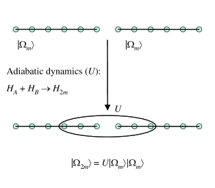
Figure 1: Illustration of the procedure to glue two copies of the ground state $|\Omega_{m}\rangle$ for $H_{m}$ together via adiabatic continuation to obtain an approximation to the ground state of $H_{2m}$.

We describe our method in a slightly more general context: we show how to glue together two systems $A$ and $B$ of $m$ and $n-m$ spins, respectively. The way we show that a good approximation $|\widetilde{\Omega}\rangle$ to the ground state $|\Omega\rangle$ can be stored efficiently is to consider the (adiabatic) dynamics of an auxiliary system $\mathcal{K}$ which is constructed in the following way. First fix $n$, the total number of spins. Next partition the chain into two contiguous blocks $A$ and $B$. Now consider the following hamiltonian

$$K=H-H_{I}$$ (2)

where $H_{I}$ is an interaction term, to be defined, which spans the boundary between the two blocks. ($H_{I}$ will not be the same as $h_{I}$, the interaction term in $H$ which spans the boundary.) If $A$ consists of the first $m$ spins, $m<n$, then $B$ consists of the last $n-m$ spins and we define $H_{I}=h_{I}+\delta\mathbb{I}$, where $\delta$ is some constant. Thus we can write $K=H_{A}+H_{B}-\delta\mathbb{I}$, where $H_{A}=\sum_{j=0}^{m-2}h_{j}$ and $H_{B}=\sum_{j=m}^{n-2}h_{j}$. We note that $K$ has a unique ground state and spectral gap $\Delta E$ because of the assumed spectral structure of the family $H_{n}$, i.e., both $H_{A}$ and $H_{B}$ belong to the family $H_{n}$ ($H_{A}\approx H_{m}$ and $H_{B}\approx H_{n-m}$). We set the constant $\delta$ so that the ground-state energy of $K$ is zero. (Recall that we’ve already set the zero of energy by requiring the ground-state energy of $H$ is $0$.)

Now we construct a new system $\mathcal{C}^{\prime}$ whose hilbert space is a direct sum of two copies of the old hilbert space. The hamiltonian $L$ for the new system is a direct sum of $H$ and $K$:

$$L=\left(\begin{matrix}H&0\\ 0&K\end{matrix}\right).$$ (3)

The hilbert space for our new system is thus given by $\mathcal{H}_{\mathcal{C}^{\prime}}=\bigotimes_{j=0}^{n}\mathbb{C}^{2}$. We think of this hilbert space as that of the original chain $\mathcal{C}$ of $n$ spins with an extra spin, which we call $C^{\prime}$, that lives between spins $m-1$ and $m$. Thus we can write $L$ as $L=\mathbb{I}_{C^{\prime}}\otimes K+\left(\frac{\mathbb{I}_{C^{\prime}}+\sigma^{z}_{C^{\prime}}}{2}\right)\otimes H_{I}$, where $\sigma^{z}=(\begin{smallmatrix}1&0\\ 0&-1\end{smallmatrix})$.

We next observe, by the assumed properties of $H$ and $K$, that the spectrum $\operatorname{sp}(L)$ of $L$ has the following structure. Firstly, the hamiltonian $L$ has a doubly degenerate ground eigenspace spanned by the vectors $\{|0\rangle|\Omega_{H}\rangle,|1\rangle|\Omega_{K}\rangle\}$, where $|\Omega_{H}\rangle$ (respectively, $|\Omega_{K}\rangle$) is the ground state of $H$ (respectively, $K$). The hamiltonian $L$ then has a gap $\Delta E$ which is larger than some constant, irrespective of the number $n$ of spins.

To construct our final auxiliary system $\mathcal{K}$ we consider the parameter-dependent hamiltonian

$$M(\theta)=L+\kappa V_{C^{\prime}}(\theta)\otimes\mathbb{I}_{\mathcal{C}}$$ (4)

where

$$V(\theta)=(\sin(\theta)|0\rangle-\cos(\theta)|1\rangle)(\sin(\theta)\langle 0|-\cos(\theta)\langle 1|).$$ (5)

We note that $V(\theta)$ is positive semidefinite and it acts nontrivially only on the auxiliary spin. Thus, to find the ground state of $M(\theta)$ we can restrict our attention to subspace spanned by $\{|0\rangle|\Omega_{H}\rangle,|1\rangle|\Omega_{K}\rangle\}$.

The addition of the operator $V(\theta)$ will perturb all of the eigenvectors of $L$. However, by Weyl’s perturbation Theorem Bhatia (1997), as long as $\kappa<\frac{\Delta E}{2}$ the operator $V(\theta)$ will not mix the ground subspace of $L$ with the remaining eigenvectors of $M(\theta)$; this subspace will always be separated by a gap from the rest of the spectrum. Furthermore, the subspace itself is unchanged: only the eigenvectors within this subspace change under the addition of $V(\theta)$. Thus we fix $\kappa=\frac{\Delta E}{4}$, so $M(\theta)=L+\frac{\Delta E}{4}V(\theta)$. The matrix elements of $V(\theta)$ in the ground eigenspace of $L$ are given by $V_{jk}(\theta)=\langle\psi_{j}|V(\theta)|\psi_{k}\rangle$, $j,k\in\{0,1\}$, where $|\psi_{0}\rangle=|0\rangle|\Omega_{H}\rangle$ and $|\psi_{1}\rangle=|1\rangle|\Omega_{K}\rangle$:

$$V_{jk}(\theta)=\begin{pmatrix}\sin^{2}(\theta)&-\sin(\theta)\cos(\theta)\overline{x}\\ -\sin(\theta)\cos(\theta){x}&\cos^{2}(\theta)\end{pmatrix}.$$ (6)

The two eigenvalues and eigenvectors of this matrix correspond to the ground state and first excited state of $M(\theta)$. The corresponding gap of $V(\theta)$ is

$$\Delta(\theta)=\sqrt{1-4\sin^{2}(\theta)\cos^{2}(\theta)(1-|x|^{2})},$$ (7)

which has a minimum value equal to $|x|$ at $\theta=\frac{\pi}{4}$, where $x$ is defined by Eq. (1).

We think of the $V(\theta)$ contribution in $M(\theta)$ as polarising the system $L$ so it has a unique gapped ground state

$$|\Omega_{M}(\theta)\rangle=\cos(\theta)|0\rangle|\Omega_{H}\rangle+\sin(\theta)|1\rangle|\Omega_{K}\rangle.$$ (8)

By the discussion in the previous paragraph the gap above this ground state is always larger than $\frac{\Delta E|x|}{4}$.

The idea behind our proof is now simple to state. We begin with the system $\mathcal{K}$ in the ground state $|\Omega_{M}(0)\rangle=|0\rangle_{C^{\prime}}|\Omega_{A}\rangle|\Omega_{B}\rangle$ of $M(0)$ and adiabatically vary $\theta$ from $0$ to $\frac{\pi}{2}$. The resulting ground state is $|1\rangle_{C^{\prime}}|\Omega_{H}\rangle$. This is a product state between the original chain $\mathcal{C}$ and $C^{\prime}$. We then discard the ancilla spin $C^{\prime}$ to obtain the ground state of $\mathcal{C}$. We approximate this exact adiabatic evolution with a unitary operator which acts nontrivially only on a small set $\Lambda$ of spins across the boundary between $A$ and $B$.

IV Approximating the adiabatic dynamics

The adiabatic evolution of the ground state $|\Omega_{M}(\theta)\rangle=\mathcal{U}(\theta;0)|\Omega_{M}(0)\rangle$ of $M(\theta)$ is generated by the solution of the differential equation

$$\frac{d}{d\theta}\mathcal{U}(\theta;0)=[\Omega_{M}^{\prime}(\theta),\Omega_{M}(\theta)]\mathcal{U}(\theta;0),$$ (9)

where $\Omega_{M}(\theta)=|\Omega_{M}(\theta)\rangle\langle\Omega_{M}(\theta)|$. This is an example of an exact adiabatic evolution (see App. A for more discussion of exact adiabatic evolution).

We approximate the exact adiabatic evolution $\mathcal{U}(\theta)$ by quasi-adiabatic evolution which, for us, is defined by the solution of the differential equation

$$\frac{d}{ds}\mathcal{V}(s;0)=\\ i\int_{-\infty}^{\infty}\chi_{\gamma}(t)\left(\int_{0}^{t}\tau_{u}^{M(s)}\left(\frac{\partial M(s)}{\partial s}\right)du\right)dt\,\mathcal{V}(s;0),$$ (10)

where

$$\chi_{\gamma}(t)=\frac{e^{-\frac{t^{2}}{2\gamma^{2}}}}{\sqrt{2\pi}\gamma},$$ (11)

and $\gamma$ is some constant to be set later, and $\tau_{t}^{M}(N)=e^{itM}Ne^{-itM}$. (See App. A for a discussion of quasi-adiabatic evolution and related adiabatic-like evolutions.)

The infinitesimal generator

$$k(s)=\int_{-\infty}^{\infty}\chi_{\gamma}(t)\left(\int_{0}^{t}\tau_{u}^{M(s)}\left(\frac{\partial M(s)}{\partial s}\right)du\right)dt$$ (12)

of quasi-adiabatic evolution is an operator which is approximately local in a region $\Lambda_{j}=\{l\,|\,d(l,C^{\prime})\leq j\}$ of $2j+1$ sites surrounding the boundary between $A$ and $B$. The way to see this intuitively is to recognise that $\frac{\partial M(s)}{\partial s}$ is strictly local in the region $\Lambda_{1}$, and the operator $\tau_{u}^{M(s)}\left(\frac{\partial M(s)}{\partial s}\right)$ is a local operator evolved according to a local hamiltonian for some time which is approximately less than some constant $\gamma$. We make this intuition precise by applying a Lieb-Robinson bound Lieb and Robinson (1972); Hastings (2004); Nachtergaele and Sims (2006); Hastings and Koma (2006) (see Osborne (2006b) for a simple direct proof). The Lieb-Robinson bound reads (for a system with hamiltonian $H$)

$$\|[\tau_{t}^{H}(A),B]\|\leq|Y|e^{-vd(x,Y)}(e^{\kappa|t|}-1),$$ (13)

for any two norm-$1$ operators $A$ acting on site $x$ and $B$ acting on a subset ${Y}$ of sites, with $\{x\}\cap Y=\emptyset$, which are separated by a distance $d(x,Y)$. The constants $v$ and $\kappa$ are independent of $n$ and depend only on $\|h\|$, which is an $O(1)$ constant.

What we do is define

$$k_{\alpha}(s)=\mathcal{F}_{s}^{M_{\Lambda_{\alpha}}(s)}\left(\frac{\partial M(s)}{\partial s}\right),$$ (14)

where

$$\mathcal{F}_{s}^{M_{\Lambda_{\alpha}}(s)}(\cdot)=\int_{-\infty}^{\infty}\chi_{\gamma}(t)\left(\int_{0}^{t}\tau_{u}^{M_{\Lambda_{\alpha}}(s)}(\cdot)\,du\right)dt,$$ (15)

with $M_{\Lambda_{\alpha}}(s)=\mathbb{I}_{C^{\prime}}\otimes H_{\Lambda_{\alpha}}+\frac{\Delta E}{4}V(s)+\left(\frac{\mathbb{I}_{C^{\prime}}+\sigma^{z}_{C^{\prime}}}{2}\right)\otimes H_{I}$ and

$$H_{\Lambda_{\alpha}}=\sum_{{j}\in\Lambda_{\alpha}}h_{{j}},$$ (16)

where $h_{j}=\mathcal{T}^{j}(h)$. Obviously $k_{\alpha}(s)$ has support $\operatorname{supp}(k_{\alpha}(s))=\Lambda_{\alpha}$.

We want to show that the quasi-adiabatic dynamics generated by $k_{\alpha}(s)$:

$$\frac{d}{ds}\mathcal{V}_{\Lambda_{\alpha}}(s;0)=ik_{\alpha}(s)\mathcal{V}_{\Lambda_{\alpha}}(s;0),$$ (17)

are close to the quasi-adiabatic dynamics $\mathcal{V}(t;0)$ generated by $k(s)$. We do this by exploiting the inequality

$$\|\mathcal{V}(t;0)-\mathcal{V}_{\Lambda_{\alpha}}(t;0)\|\leq\int_{0}^{|t|}\|k(s)-k_{{\alpha}}(s)\|ds,$$

which is proved, for example, by exploiting the Lie-Trotter expansion.

We now show how the Lieb-Robinson bound provides an estimate on the decay of $\|k_{\alpha}(s)\|$. Consider

$$\begin{aligned} &\|k(s)-k_{\alpha}(s)\|=\\ &\left\|\int_{-\infty}^{\infty}\chi_{\gamma}(t)\left(\int_{0}^{t}\left(\tau_{u}^{M(s)}(m^{\prime})-\tau_{u}^{M_{\Lambda_{\alpha}}(s)}(m^{\prime})\right)du\right)dt\right\|\\ &\leq 2\int_{0}^{\infty}|\chi_{\gamma}(t)|\left(\int_{0}^{t}\left\|\tau_{u}^{M(s)}(m^{\prime})-\tau_{u}^{{M_{\alpha}}(s)}(m^{\prime})\right\|du\right)dt\\ &\leq 2\int_{0}^{\infty}|\chi_{\gamma}(t)|\left(\int_{0}^{t}\min\{2\|m^{\prime}\|,c\alpha^{2}\Delta Ee^{\kappa|u|-v\alpha}\}du\right)dt\\ &\lesssim\frac{\alpha^{2}\Delta E}{\gamma}\int_{0}^{c\alpha}|\chi_{\gamma}(t)|e^{\kappa|t|-v\alpha}dt+\Delta E\int_{c\alpha}^{\infty}|\chi_{\gamma}(t)||t|dt\\ &\lesssim\frac{\alpha^{2}\Delta E}{\gamma}\int_{0}^{c\alpha}e^{\kappa t-v\alpha}dt+\Delta E\int_{c\alpha}^{\infty}\frac{e^{-\frac{t^{2}}{2\gamma^{2}}}}{\sqrt{2\pi}\gamma}|t|dt\\ &\lesssim\frac{\alpha^{2}\Delta E}{\gamma}e^{(\kappa c-v)\alpha}+{\gamma\Delta E}e^{-\frac{c^{2}\alpha^{2}}{2\gamma^{2}}},\end{aligned}$$ (18)

where $m^{\prime}=\frac{\partial M(s)}{\partial s}=\frac{\Delta E}{4}\frac{\partial V(s)}{\partial s}$, and in the first line we applied the triangle inequality, in the second line we applied the Lieb-Robinson bound, and in the third line we’ve broken the integral into two pieces and applied the different regimes of the Lieb-Robinson bound separately with $c$ some constant and we’ve used the fact that $\|m^{\prime}\|\lesssim\Delta E$. Thus, by choosing $c<v/\kappa$ we see that $\|k(s)-k_{\alpha}(s)\|$ is decaying exponentially fast in $\alpha$ for $\alpha\gtrsim\gamma$.

Thus we learn that the quasi-adiabatic dynamics $\mathcal{V}(\frac{\pi}{2};0)$ are exponentially close (in operator norm) to a unitary operator $\mathcal{V}^{[1]}_{\Lambda_{\alpha}}(\frac{\pi}{2};0)$ which acts nontrivially on only the region $\Lambda_{\alpha}$.

In order to complete our discussion and show that the state $\mathcal{V}^{[1]}_{\Lambda_{\alpha}}(\frac{\pi}{2};0)|\Omega(0)\rangle$ is close to $|\Omega_{H}\rangle=\mathcal{U}(\frac{\pi}{2};0)|\Omega(0)\rangle$ we apply the triangle inequality to bound

$$\||\Omega_{H}\rangle-\mathcal{V}^{[1]}_{\Lambda_{\alpha}}\left(\frac{\pi}{2};0\right)|\Omega(0)\rangle\|\leq\||\Omega_{H}\rangle-\mathcal{V}\left(\frac{\pi}{2};0\right)|\Omega(0)\rangle\|+\\ \|\mathcal{V}\left(\frac{\pi}{2};0\right)|\Omega(0)\rangle-\mathcal{V}^{[1]}_{\Lambda_{\alpha}}\left(\frac{\pi}{2};0\right)|\Omega(0)\rangle\|$$ (19)

We use Eq. (58) from the appendix to bound the first term and Eq. (18) to bound the second term:

$$\||\Omega_{H}\rangle-\mathcal{V}^{[1]}_{\Lambda_{\alpha}}\left(\frac{\pi}{2};0\right)|\Omega(0)\rangle\|\lesssim\frac{e^{-{2\gamma^{2}|x|^{2}\Delta E^{2}}}}{|x|\Delta E}+\gamma\Delta Ee^{-\frac{\kappa\gamma}{v}},$$ (20)

so that $\gamma\gtrsim\frac{1}{|x|\Delta E}$ is sufficient to ensure that the approximation is exponentially small (in $\gamma$).

With the choice $\alpha\gtrsim\gamma\gtrsim\frac{1}{|x|\Delta E}$ we find that the width of the region $\Lambda_{\alpha}$ that the unitary operator $\mathcal{V}^{[1]}_{\Lambda_{\alpha}}$ acts on is given by $\frac{c}{|x|\Delta E}$, where $c$ is some constant.

To conclude our discussion we now show how to iteratively use the procedure we’ve described in the previous paragraphs to construct an approximation to the ground state $|\Omega_{H_{n}}\rangle$ of $H_{n}$ which can be stored (as a FCS) with resources scaling as a polynomial in $n$.

Our first step is to start with a system $A_{1}B_{1}$ which consists of two copies $A_{1}$ and $A_{2}$ of the chain $\mathcal{C}_{m}$ on $m$ sites with $m\gtrsim\frac{c}{|x|\Delta E}$. The hamiltonian for this system is given by

$$K_{m}=H_{m}\otimes\mathbb{I}_{B_{1}}+\mathbb{I}_{A_{1}}\otimes H_{m}-\delta_{m}\mathbb{I}.$$ (21)

This system has a ground state equal to $|\Omega_{m}\rangle|\Omega_{m}\rangle$. We then follow the procedure described above, namely, adjoining an ancilla spin $C^{\prime}$ between the two blocks, and then applying the approximate adiabatic evolution $\mathcal{V}^{[1]}_{\Lambda_{\alpha}}$ to yield an approximation $\mathcal{V}^{[1]}_{\Lambda_{\alpha}}|\Omega_{m}\rangle|\Omega_{m}\rangle$ to the ground state $|\Omega_{2m}\rangle$.

We next iterate this procedure: we use two copies of the approximation $\mathcal{V}^{[1]}_{\Lambda_{\alpha}}|\Omega_{m}\rangle|\Omega_{m}\rangle$ to approximate the state $|\Omega_{2m}\rangle|\Omega_{2m}\rangle$. This is the ground state of a new system $A_{2}B_{2}$ whose hamiltonian is given by

$$K_{2m}=H_{2m}\otimes\mathbb{I}_{B_{2}}+\mathbb{I}_{A_{2}}\otimes H_{2m}-\delta_{2m}\mathbb{I}.$$ (22)

By the discussion above, we find that this hamiltonian is adiabatically connected to $H_{4m}$. Because we are using an approximation $|\Omega_{2m}^{\prime}\rangle=\mathcal{V}^{[1]}_{\Lambda_{\alpha}}|\Omega_{m}\rangle|\Omega_{m}\rangle$ for $|\Omega_{2m}\rangle$ we must account for the error that arises when we take two copies of our approximation:

$$\begin{split}\||\Omega_{2m}\rangle|\Omega_{2m}\rangle-|\Omega_{2m}^{\prime}\rangle|\Omega_{2m}^{\prime}\rangle\|&\leq 2\|(|\Omega_{2m}\rangle-|\Omega_{2m}^{\prime}\rangle)|\Omega_{2m}\rangle\|\\ &=2\||\Omega_{2m}\rangle-\mathcal{V}^{[1]}_{\Lambda_{\alpha}}|\Omega_{m}\rangle|\Omega_{m}\rangle\|\\ &\leq 2\frac{e^{-{2\gamma^{2}|x|^{2}\Delta E^{2}}}}{|x|\Delta E}+2\gamma\Delta Ee^{-\frac{\kappa\gamma}{v}}\end{split}$$ (23)

Finally, using this upper bound we can compute the error between $|\Omega_{4m}\rangle$ and our approximation (obtained from approximating the adiabatic continuation from $|\Omega_{2m}\rangle|\Omega_{2m}\rangle$ to $|\Omega_{4m}\rangle$):

$$\||\Omega_{4m}\rangle-\mathcal{V}^{[2]}_{\Lambda_{\alpha}}|\Omega_{2m}^{\prime}\rangle)|\Omega_{2m}^{\prime}\rangle\|\leq 2\epsilon(\gamma)+\epsilon(\gamma),$$ (24)

where we’ve defined

$$\epsilon(\gamma)=\frac{e^{-{2\gamma^{2}|x|^{2}\Delta E^{2}}}}{|x|\Delta E}+\gamma\Delta Ee^{-\frac{\kappa\gamma}{v}}.$$ (25)

To obtain an approximation to the ground state $|\Omega_{n}\rangle$ of $H_{n}$ we iterate the above procedure $\lceil\log_{2}(n/m)\rceil$ times. The error resulting from applying the above procedure is given by

$$\frac{n}{m}\epsilon(\gamma)=\frac{n}{m}\left(\frac{e^{-{2\gamma^{2}|x|^{2}\Delta E^{2}}}}{|x|\Delta E}+\gamma\Delta Ee^{-\frac{\kappa\gamma}{v}}\right).$$ (26)

If we fix some prespecified error $\epsilon$ and demand that our approximation satisfies $\||\Omega_{n}\rangle-|\Omega_{n}^{\prime}\rangle\|\leq\epsilon$ then we need that

$$\gamma\geq\max\left\{\frac{c}{|x|\Delta E},c^{\prime}\log\left(\frac{n}{\epsilon}\right)\right\},$$ (27)

where $c$ and $c^{\prime}$ are constants that only depend on $\|h\|$. Hence, we learn that, similarly, the unitary operators $\mathcal{V}^{[k]}_{\Lambda_{\alpha}}(\frac{\pi}{2})$ that we apply at each stage $k$ act on a collection of $\alpha\geq c^{\prime\prime}\gamma$ spins, with $c^{\prime\prime}$ some constant which only depends on $\|h\|$.

After applying the iterative procedure described above we end up with the following representation for our approximation to $|\Omega_{n}\rangle$:

$$|\Omega_{n}\rangle=\mathcal{W}|\Omega_{m}\rangle|\Omega_{m}\rangle\cdots|\Omega_{m}\rangle$$ (28)

where

$$\mathcal{W}=\mathcal{V}_{\Lambda_{\alpha}(1)}\mathcal{V}_{\Lambda_{\alpha}(2)}\cdots\mathcal{V}_{\Lambda_{\alpha}(\lceil\log_{2}(n/m)\rceil-1)},$$ (29)

with $\Lambda_{\alpha}(j)=\{k\,|\,d(k,mj)\leq\alpha\}$.

The representation Eq. (28) is equivalent Osborne (2006c); Verstraete and Cirac (2006) to a finitely correlated state requiring a number of degrees of freedom which scale as $n2^{c|\Lambda_{\alpha}|}$, where $c$ is some constant. Alternatively, it is clear that the representation Eq. (28) is already in a form useful for extracting local properties: the expectation values of local operators such as correlators are easy to compute using the representation Eq. (28). Finally, it is worth noting that our representation is also exactly in the form of a simple instance of the multiscale entanglement renormalisation ansatz introduced in Vidal (2005).

V Conclusions and future directions

In this paper we have shown how a class of noncritical 1D quantum spin systems are adiabatically connected to a 1D quantum spin system of $\frac{n}{m}$ noninteracting quantum spins with local dimension $2^{m}$. As long as $m\gg\max\left\{\frac{c}{|x|\Delta E},c^{\prime}\log\left(\frac{n}{\epsilon}\right)\right\}$, where $c$ and $c^{\prime}$ are constants which only depend on $\|h\|$, then the ground state $|\Omega_{n}\rangle$ of $H_{n}$ can be approximated efficiently. This result bears a superficial resemblance to a naive application of real-space renormalisation: in real-space renormalisation one argues that blocks of $\frac{c}{\Delta E}$ spins should be effectively noninteracting. (I.e., after $\log(\frac{c}{\Delta E})$ renormalisation group transformations we should be very close to a trivial fixed point.) While this intuition is clear it seems to be extremely challenging to put this intuition on a rigourous footing.

One question presents itself at this point: for noncritical spin systems with a gap $\Delta E$ do the boundary effects persist only a distance $\frac{c}{\Delta E}$ into the interior of the system? Despite the plausibility of this statement we’ve been unable to prove it; there are many counterexample systems which appear to ruin the most obvious approaches.

Appendix A Errors in approximations of adiabatic dynamics

The dynamics generated by the adiabatic evolution of a quantum system is an important paradigm in the study of quantum mechanics. One question which is particularly pertinent for the simulation of quantum systems is: can adiabatic evolution be simulated by the time-dependent dynamics of some (possibly different) quantum system? In the case of adiabatic evolution the answer is yes: one method is to just slowly turn on the interactions on a timescale which is small compared to the gap of the system. While this is an entirely satisfactory solution in and of itself one limitation lies in the error of this approximation; when adiabatic dynamics is simulated via this method the error decreases as an inverse polynomial in the timescale $T$ of the slowly changing dynamics Reichardt (2004). Thus we are inspired to search for methods which provide better error scaling. One such method is provided by quasi-adiabatic evolution Wen and Hastings (2005) (see also Avron and Elgart (1999)). In this case we find that the error scales exponentially as a function of the timescale $T$ set by the gap of the system. In this appendix we show this exponential scaling. Our discussion is set in the wider context of “adiabatic” evolutions whose differential generators can be arbitrary.

The framework we describe in this section to discuss quasi-adiabatic evolutions is similar to that introduced by Avron and Elgart (1999) and Wen and Hastings (2005).

A.1 Quasi-adiabatic evolutions

In this subsection we introduce a general framework to describe “adiabatic”-like evolutions for quantum systems.

We consider adiabatic quantum evolution generated by a parameter-dependent hamiltonian $H(s)$ as $s$ is varied adiabatically from $s=0$ to $s=1$. Thus we would like to understand the ground state $|\Omega(s)\rangle$ of $H(s)$. We do this by setting up a differential equation for $|\Omega(s)\rangle$:

$$\frac{d}{ds}|\Omega(s)\rangle=P^{\prime}(s)|\Omega(s)\rangle,$$ (30)

where $P^{\prime}(s)=\frac{d}{ds}(|\Omega(s)\rangle\langle\Omega(s)|)$ and we’ve set phases endnote30 so that $\langle\Omega^{\prime}(s)|\Omega(s)\rangle=0$. Because $P^{\prime}(s)$ is not antihermitian the dynamics generated by this equation are not unitary.

There are at least two ways to set up differential equations for $|\Omega(s)\rangle$ which do generate unitary dynamics. The first is via exact adiabatic evolution (see Avron et al. (1987, 1993) for a rigourous discussion of rather general results about exact adiabatic evolution):

$$\frac{d}{ds}|\Omega(s)\rangle=-[P(s),P^{\prime}(s)]|\Omega(s)\rangle.$$ (31)

Because of the gap condition on $H(s)$, the “hamiltonian” $[P(s),P^{\prime}(s)]$ for this dynamics is given by first-order stationary perturbation theory:

$$[P(s),P^{\prime}(s)]=|\Omega(s)\rangle\langle\Omega(s)|\frac{\partial H(s)}{\partial s}\frac{\mathbb{I}}{\Omega(s)\mathbb{I}-H(s)}-\\ \frac{\mathbb{I}}{\Omega(s)\mathbb{I}-H(s)}\frac{\partial H(s)}{\partial s}|\Omega(s)\rangle\langle\Omega(s)|,$$ (32)

where $\Omega(s)$ is the ground-state energy of $H(s)$, and we define $\frac{\mathbb{I}}{\Omega(s)\mathbb{I}-H(s)}$ via the Moore-Penrose inverse: $\frac{\mathbb{I}}{\Omega(s)\mathbb{I}-H(s)}|\Omega(s)\rangle=0$.

We now define an infinitesimal generator for a quantum evolution which is meant to simulate the adiabatic evolution. We begin by specifying a function $\chi_{\gamma}(t)$ which is an even real function whose fourier transform $\widehat{\chi}_{\gamma}$ is decaying rapidly outside some region $[-\gamma,\gamma]$, and which is normalised so that $\widehat{\chi}_{\gamma}(0)=1$. We use this function to create an operator $Q(s)$ which is meant to approximate $P(s)$:

$$Q(s)=\int_{-\infty}^{\infty}\chi_{\gamma}(t)e^{-it\Omega(s)}e^{itH(s)}dt,$$ (33)

The following formula for $Q(s)$ may be verified by writing $e^{itH}$ in its eigenbasis and exploiting the $L_{2}$ unitarity of the fourier transform:

$$Q(s)=\sum_{j=0}^{2^{n}-1}\widehat{\chi}_{\gamma}(E_{j}(s)-\Omega(s))|E_{j}(s)\rangle\langle E_{j}(s)|$$ (34)

How close is $Q(s)$ to $P(s)$? We measure distance in operator norm:

$$\|Q(s)-P(s)\|=\sup_{z\in\operatorname{sp}(H(s))\setminus\Omega(s)}\widehat{\chi}_{\gamma}(z-\Omega(s)).$$ (35)

This formula shows us that, in the case where $H(s)$ has a gap $\Delta E(s)\geq\Delta$, $Q(s)$ is close $P(s)$ in operator norm as long as $|\widehat{\chi}_{\gamma}(z)|$ decays rapidly for $|z|\gtrsim\Delta$.

In the case that $\chi_{\gamma}(t)$ is an even real function whose fourier transform $\widehat{\chi}_{\gamma}$ is $C^{\infty}$, has compact support in $[-\gamma,\gamma]$, and is normalised so that $\widehat{\chi}_{\gamma}(0)=1$ with $\gamma<\Delta$ to ensure that only the ground state appears on the RHS of (33) we can recover exact adiabatic dynamics: we first use the Duhamel formula

$$\frac{d}{ds}e^{itH(s)}=i\int_{0}^{t}e^{i(t-u)H(s)}\frac{\partial H(s)}{\partial s}e^{iuH(s)}du,$$

to rewrite (30):

$$\frac{d}{ds}|\Omega(s)\rangle=-i\frac{d\Omega(s)}{ds}\int_{-\infty}^{\infty}t\chi_{\gamma}(t)dt|\Omega(s)\rangle+i\int_{-\infty}^{\infty}\chi_{\gamma}(t)e^{-it\Omega(s)}\left(\int_{0}^{t}\tau_{u}^{H(s)}\left(\frac{\partial H(s)}{\partial s}\right)du\right)e^{itH(s)}dt|\Omega(s)\rangle.$$ (36)

Using the fact that $\chi_{\gamma}(t)$ is an even function of $t$ and cancelling phases we obtain

$$\frac{d}{ds}|\Omega(s)\rangle=i\int_{-\infty}^{\infty}\chi_{\gamma}(t)\left(\int_{0}^{t}\tau_{u}^{H(s)}\left(\frac{\partial H(s)}{\partial s}\right)du\right)dt|\Omega(s)\rangle.$$ (37)

By integrating this expression for $\frac{d}{ds}|\Omega(s)\rangle$ in the energy eigenbasis of $H(s)$ and using the assumed gap structure one can find that this expression is equivalent to the usual expression obtained from first-order perturbation theory:

$$\frac{d}{ds}|\Omega(s)\rangle=\frac{\mathbb{I}}{\Omega(s)\mathbb{I}-H(s)}\frac{\partial H(s)}{\partial s}|\Omega(s)\rangle.$$ (38)

We use the form (37) to deduce a hermitian infinitesimal generator

$$K(s)=\int_{-\infty}^{\infty}\chi_{\gamma}(t)\left(\int_{0}^{t}\tau_{u}^{H(s)}\left(\frac{\partial H(s)}{\partial s}\right)du\right)dt$$ (39)

of exact adiabatic evolution. Thus we find

$$|\Omega(s)\rangle=\mathcal{T}e^{i\int^{t}_{0}K(s)\,ds}|\Omega(0)\rangle=\mathcal{U}(t;0)|\Omega(0)\rangle$$ (40)

where we define

$$\mathcal{U}(t;0)=\mathcal{T}e^{i\int^{t}_{0}K(s)\,ds}.$$ (41)

It is now easy to guess a form for the infinitesimal generator $L_{\chi_{\gamma}}(s)$ which is meant to approximate exact adiabatic dynamics: we just allow the function $\chi_{\gamma}(s)$ in (39) to be arbitrary:

$$L_{\chi_{\gamma}}(s)=\int_{-\infty}^{\infty}\chi_{\gamma}(t)\left(\int_{0}^{t}\tau_{u}^{H(s)}\left(\frac{\partial H(s)}{\partial s}\right)du\right)dt.$$ (42)

(We drop the subscript on $L_{\chi_{\gamma}}(s)$ from now on.) The corresponding dynamics are obtained by integration:

$$\mathcal{V}(t;0)=\mathcal{T}e^{i\int^{t}_{0}L(s)\,ds}.$$ (43)

We call the dynamics $\mathcal{V}(t;0)$ a quasi-adiabatic evolution.

With the definition (43) of quasi-adiabatic evolution we now define the (time-dependent) state $|\Phi(t)\rangle$:

$$|\Phi(t)\rangle=\mathcal{V}(t;0)|\Omega(0)\rangle.$$ (44)

The idea is that $|\Phi(t)\rangle$ should be very close to $|\Omega(t)\rangle$ as long as $\|Q(s)-P(s)\|$ is small. We make this rigourous in the next section.

A.2 Error in quasi-adiabatic evolution

In this section we study the error $\delta(t)=\||\Phi(t)\rangle-|\Omega(t)\rangle\|$ between the exact ground state of $H(s)$ and the state $|\Phi(t)\rangle$ generated by quasi-adiabatic evolution.

To get started on an upper bound for $\delta(t)$ we define

$$|\delta(t)\rangle=|\Omega(0)\rangle-\mathcal{V}(t;0)^{\dagger}|\Omega(t)\rangle=|\Omega(0)\rangle-\mathcal{V}(0;t)|\Omega(t)\rangle.$$ (45)

It is easy to see, using the unitary invariance of $\|\cdot\|$, that $\delta(t)=\||\delta(t)\rangle\|$.

We use the fundamental theorem of calculus to write $|\delta(t)\rangle$ as

$$|\delta(t)\rangle=\int_{0}^{t}\frac{d}{ds}\left(\mathcal{V}(s;0)^{\dagger}|\Omega(s)\rangle\right)\,ds.$$ (46)

Now we use the definitions of $\frac{d}{ds}|\Omega(s)\rangle$ and $\frac{d}{ds}\mathcal{V}(s;0)$ to find

$$|\delta(t)\rangle=\int_{0}^{t}\left(-i\mathcal{V}(s;0)^{\dagger}L(s)|\Omega(s)\rangle+\mathcal{V}(s;0)^{\dagger}\frac{\mathbb{I}}{\Omega(s)\mathbb{I}-H(s)}\frac{\partial H(s)}{\partial s}|\Omega(s)\rangle\right)\,ds.$$ (47)

Thus, using the triangle inequality and unitary invariance of $\|\cdot\|$, we find

$$\delta(t)=\||\delta(t)\rangle\|\leq\\ \int_{0}^{t}\left\|iL(s)|\Omega(s)\rangle-\frac{\mathbb{I}}{\Omega(s)\mathbb{I}-H(s)}\frac{\partial H(s)}{\partial s}|\Omega(s)\rangle\right\|\,ds.$$ (48)

To make some headway on this expression we derive an expression for $L(s)|\Omega(s)\rangle$:

$$iL(s)|\Omega(s)\rangle=\\ i\int_{-\infty}^{\infty}\chi_{\gamma}(t)\left(\int_{0}^{t}\tau_{u}^{H(s)}\left(\frac{\partial H(s)}{\partial s}\right)du\right)dt|\Omega(s)\rangle.$$ (49)

By integration, we find

$$iL(s)|\Omega(s)\rangle=\\ \left(\frac{\widehat{\chi}_{\gamma}(H(s)-\Omega(s)\mathbb{I})}{H(s)-\Omega(s)\mathbb{I}}+\frac{\mathbb{I}}{\Omega(s)\mathbb{I}-H(s)}\right)\frac{\partial H(s)}{\partial s}|\Omega(s)\rangle,$$ (50)

where we define, as before, $\frac{\mathbb{I}}{\Omega(s)\mathbb{I}-H(s)}$ via the Moore-Penrose inverse: $\frac{\mathbb{I}}{\Omega(s)\mathbb{I}-H(s)}|\Omega(s)\rangle=0$, and we define the operator $\widehat{\chi}_{\gamma}(H(s)-\Omega(s)\mathbb{I})$ using the holomorphic function calculus Kadison and Ringrose (1997):

$$\widehat{\chi}_{\gamma}(H(s)-\Omega(s)\mathbb{I})=\sum_{j=0}^{2^{n}-1}\widehat{\chi}_{\gamma}(E_{j}(s)-\Omega(s))|E_{j}(s)\rangle\langle E_{j}(s)|.$$ (51)

Substituting this expression for $iL(s)|\Omega(s)\rangle$ into (48) we find

$$\delta(t)\leq\int_{0}^{t}\left\|\frac{\widehat{\chi}_{\gamma}(H(s)-\Omega(s)\mathbb{I})}{H(s)-\Omega(s)\mathbb{I}}\frac{\partial H(s)}{\partial s}|\Omega(s)\rangle\right\|\,ds.$$ (52)

We rewrite this as

$$\delta(t)\leq\int_{0}^{t}\sqrt{\langle\eta(s)|\left(\frac{\widehat{\chi}_{\gamma}(H(s)-\Omega(s)\mathbb{I})}{H(s)-\Omega(s)\mathbb{I}}\right)^{2}|\eta(s)\rangle}\,ds,$$ (53)

where

$$|\eta(s)\rangle=\mathcal{P}_{\text{high}}\frac{\partial H(s)}{\partial s}|\Omega(s)\rangle$$ (54)

and

$$\mathcal{P}_{\text{high}}=\sum_{j=1}^{2^{n}-1}|E_{j}(s)\rangle\langle E_{j}(s)|.$$ (55)

(Recall we are defining $\frac{\mathbb{I}}{\Omega(s)\mathbb{I}-H(s)}$ via the Moore-Penrose inverse.)

We now define $\eta(t)=\left\|\mathcal{P}_{\text{high}}\frac{\partial H(s)}{\partial s}|\Omega(s)\rangle\right\|\leq\left\|\frac{\partial H(s)}{\partial s}\right\|$ and $\eta_{*}=\sup_{s\in[0,t]}\eta(s)$ to rewrite (53) as

$$\||\delta(t)\rangle\|\leq\eta_{*}\int_{0}^{t}\left\|\frac{\widehat{\chi}_{\gamma}(H(s)-\Omega(s)\mathbb{I})}{H(s)-\Omega(s)\mathbb{I}}\right\|\,ds.$$ (56)

We also define

$$\begin{split}f(s)&=\left\|\frac{\widehat{\chi}_{\gamma}(H(s)-\Omega(s)\mathbb{I})}{H(s)-\Omega(s)\mathbb{I}}\right\|\\ &=\sup_{z\in\operatorname{sp}(H(s))\setminus\Omega(s)}\frac{\widehat{\chi}_{\gamma}(z-\Omega(s))}{z-\Omega(s)}\end{split}$$ (57)

and set $f_{*}=\sup_{s\in[0,t]}f(s)$ to obtain our final estimate

$$\||\delta(t)\rangle\|\leq\eta_{*}f_{*}.$$ (58)

The quantities $\eta_{*}$ and $f_{*}$ can be separately upper bounded. In the case of spin systems which are adiabatically evolving we can generally bound $\eta_{*}$ by $\eta_{*}\leq cn$, where $c$ is a constant and $n$ is the number of spins. For $f_{*}$: in the case that our system has a gap $\Delta$ we use the cutoff function

$$\chi_{\gamma}(t)=\frac{e^{-\frac{t^{2}}{2\gamma^{2}}}}{\sqrt{2\pi}\gamma},$$ (59)

which has fourier transform

$$\widehat{\chi}_{\gamma}(\omega)={e^{-{2\gamma^{2}\omega^{2}}}}.$$ (60)

We can now put together the gap structure of the spectrum of $H(s)$ and the fourier transform of $\chi_{\gamma}(t)$ to obtain the bound

$$f_{*}\leq\frac{e^{-{2\gamma^{2}\Delta^{2}}}}{\Delta}.$$ (61)

This expression is exponentially decaying in $\gamma$, indeed, $\gamma\gtrsim\frac{1}{\Delta}$ is sufficient to make this upper bound for $f_{*}$ arbitrarily small. Putting these two bounds for $\eta_{*}$ and $f_{*}$ together we find that, for adiabatically evolving spin systems, $\gamma\gtrsim\frac{1}{\Delta}\sqrt{\log(n)}$ is sufficient to reduce the error $\delta(t)$ until it is arbitrarily small.

It is easy to extend our discussion to systems $H(s)$ which have a continuous gapless spectrum as long as there is some bound on the growth of the density of states near the ground state Avron and Elgart (1999); Wen and Hastings (2005).

References

- Hastings (2005) M. B. Hastings, Phys. Rev. B 73, 085115 (2005), eprint cond-mat/0508554.
- Schollwöck (2005) U. Schollwöck, Rev. Modern Phys. 77, 259 (2005), eprint cond-mat/0409292.
- Verstraete and Cirac (2004) F. Verstraete and J. I. Cirac (2004), eprint cond-mat/0407066.
- Eisert (2006) J. Eisert, Phys. Rev. Lett. 62, 260501 (2006), eprint quant-ph/0609051.
- Fannes et al. (1992) M. Fannes, B. Nachtergaele, and R. F. Werner, Comm. Math. Phys. 144, 443 (1992).
- Vidal (2003) G. Vidal, Phys. Rev. Lett. 93, 040502 (2003), eprint quant-ph/0310089.
- Zwolak and Vidal (2003) M. Zwolak and G. Vidal, Phys. Rev. Lett. 93, 207205 (2003), eprint cond-mat/0406440.
- Verstraete et al. (2004) F. Verstraete, J. J. García-Ripoll, and J. I. Cirac, Phys. Rev. Lett. 93, 207204 (2004), eprint quant-ph/0406426.
- Osborne (2006a) T. J. Osborne (2006a), eprint quant-ph/0601019.
- Oliveira and Terhal (2005) R. Oliveira and B. M. Terhal (2005), eprint quant-ph/0504050.
- Kempe et al. (2004) J. Kempe, A. Kitaev, and O. Regev, in FSTTCS 2004: Foundations of software technology and theoretical computer science (Springer, Berlin, 2004), vol. 3328 of Lecture Notes in Comput. Sci., pp. 372–383, eprint quant-ph/0406180.
- Kitaev et al. (2002) A. Y. Kitaev, A. H. Shen, and M. N. Vyalyi, Classical and quantum computation, vol. 47 of Graduate Studies in Mathematics (American Mathematical Society, Providence, RI, 2002).
- Bhatia (1997) R. Bhatia, Matrix analysis (Springer-Verlag, New York, 1997).
- Lieb and Robinson (1972) E. H. Lieb and D. W. Robinson, Commun. math. Phys. 28, 251 (1972).
- Hastings (2004) M. B. Hastings, Phys. Rev. B 69, 104431 (2004), eprint cond-mat/0305505.
- Nachtergaele and Sims (2006) B. Nachtergaele and R. Sims, Commun. Math. Phys. 265, 119 (2006), eprint math-ph/0506030.
- Hastings and Koma (2006) M. B. Hastings and T. Koma, Commun. Math. Phys. 265, 781 (2006), eprint math-ph/0507008.
- Osborne (2006b) T. J. Osborne (2006b), www.lri.fr/qip06/slides/osborne.pdf.
- Osborne (2006c) T. J. Osborne, Phys. Rev. Lett. 97, 157202 (2006c), eprint quant-ph/0508031.
- Verstraete and Cirac (2006) F. Verstraete and J. I. Cirac, Phys. Rev. B 73, 094423 (2006), eprint cond-mat/0505140.
- Vidal (2005) G. Vidal (2005), eprint cond-mat/0512165.
- Reichardt (2004) B. W. Reichardt, in Proceedings of the 36th Annual ACM Symposium on Theory of Computing (ACM, New York, 2004), pp. 502–510.
- Wen and Hastings (2005) X.-G. Wen and M. B. Hastings, Phys. Rev. B 72, 045141 (2005), eprint cond-mat/0503554.
- Avron and Elgart (1999) J. E. Avron and A. Elgart, Comm. Math. Phys. 203, 445 (1999).
- Avron et al. (1987) J. E. Avron, R. Seiler, and L. G. Yaffe, Comm. Math. Phys. 110, 33 (1987).
- Avron et al. (1993) J. E. Avron, R. Seiler, and L. G. Yaffe, Comm. Math. Phys. 156, 649 (1993).
- Kadison and Ringrose (1997) R. V. Kadison and J. R. Ringrose, Fundamentals of the theory of operator algebras. Vol. I, vol. 15 of Graduate Studies in Mathematics (American Mathematical Society, Providence, RI, 1997).
- (28) By “noncritical” we mean the the Hamiltonian for the system has a spectral gap between the ground state and first-excited state which is a constant that doesn’t scale with , the number of spins.
- (29) Barbara Terhal and David DiVincenzo (private communication)
- (30) Note that this choice precludes an extension of our analysis to study Berry phases.