Bell-type inequalities for non-local resources

Abstract

We present bipartite Bell-type inequalities which allow the two partners to use some non-local resource. Such inequality can only be violated if the parties use a resource which is more non-local than the one permitted by the inequality. We introduce a family of $N$-inputs non-local machines, which are generalizations of the well-known PR-box. Then we construct Bell-type inequalities that cannot be violated by strategies that use one these new machines. Finally we discuss implications for the simulation of quantum states.

I Introduction

One of the most striking properties of quantum mechanics is non-locality. It is well known that two separated observers, each holding half of an entangled quantum state and performing appropriate measurements, share correlations which are non-local, in the sense that they violate a Bell inequality [1]. Indeed this has been demonstrated in many laboratory experiments [2]. A key feature of entanglement is that it does not allow the two distant observers to send information to each other faster than light, i.e. correlation from measurements on quantum states are no-signaling.

It is an interesting problem to quantify how powerful the non-local correlations of quantum mechanics are. In order to do that, one has to use some non-local resource. A quite natural choice is indeed classical communication. In 2003, Toner and Bacon showed that a single bit of communication is enough to reproduce the correlations of the singlet state [3]. In the last years another non-local resource, the PR-box, has also been proposed to study this problem. Introduced in 1994 by Popescu and Rohrlich [4, 5], the PR-box was then proven to be a powerful resource for information theoretic tasks, such as communication complexity [6, 7] and cryptography [8]. It was also recently suggested that the PR-box is a unit of non-locality [9]. The PR-box has the appealing feature that it is intrinsically non signaling, which is of course not the case of classical communication [10]. Note that a PR-box is a strictly weaker resource than a bit of communication [11]. Recently, Cerf et al. presented a model using a single PR-box which simulates correlations from any projective measurement on the singlet [12]. It appears very natural to extend this study to other quantum states, but this turns out to be quite difficult, even for non-maximally entangled pure states of two qubits. In a recent paper we showed a family of non-maximally entangled states, whose correlations cannot be reproduced by a single PR-box [11]. In other words, some non-maximally entangled states require a strictly larger amount of non-local resources than the maximally entangled state to be simulated. This suggests that entanglement and non-locality are different resources. To demonstrate this result we found a Bell-type inequality allowing some non-local resource; in this case a single use of a PR-box. Then it was proven that this inequality is violated by some non-maximally entangled state.

In the present paper, we introduce N-inputs bipartite non-local machines (NLM), which appear as a natural extension of the two-inputs PR-box. These machines, denoted $PR_{N}$, have a nice connection to a family of N-settings Bell inequalities known as $I_{NN22}$ [13], similar to the one that relates the PR-box to the Clauser-Horne-Shimony-Holt (CHSH) inequality [14]:

CHSH $$\Rightarrow$$ PR-box (1)

$$I_{NN22}\quad \Rightarrow \quad PR_{N}\quad.$$ (2)

In fact, the structure of the N-inputs NLM can be directly deduced from the corresponding $I_{NN22}$ inequality. Then we present a family of N-settings inequalities, $M_{NN22}$, which allow one use of $PR_{N-1}$ machine. Again, the structure of these new inequalities is easily deduced from the structure of the $I_{NN22}$ inequalities, i.e.

$$I_{NN22}\quad \Rightarrow \quad M_{NN22}\quad.$$ (3)

Thus a nice construction appears: for any number of settings $N$, we have a Bell inequality $I_{NN22}$ and the related NLM, $PR_{N}$, which reaches the upper (no-signaling) bound of the inequality. Adding one setting we find another inequality, $M_{(N+1)(N+1)22}$, that cannot be violated by strategies which require a single use of $PR_{N}$.

The organization of the paper is as follows. In Section II we present the mathematical tools and introduce the notations by reviewing the simplest case of two settings on each side. The link between the PR-box and the CHSH inequality is pointed out. Section III is devoted to the case of three settings: we introduce a three-setting NLM and study an inequality for a single use of a PR-box. In Section IV, the construction of Section III is extended to the case N settings. Section V concludes the paper by reviewing the main results about Bell inequalities with and without resources. Our present work is then clearly situated in this context.

II Tools

Let’s consider a typical Bell test scenario. Two distant observers, Alice and Bob, share some quantum state. Each of them chooses between a set of measurements (settings) $\{A_{i}\}_{i=1..N_{A}}$, $\{B_{j}\}_{j=1..N_{B}}$. The result of the measurement is noted $r_{A}$, $r_{B}$. Here we will focus on dichotomic observables and we will restrict Alice and Bob to use the same number of settings, i.e. $r_{A,B}\in\{0,1\}$ and $N_{A}=N_{B}\equiv N$. An ”experiment” is fully characterized by the family of $4N^{2}$ probabilities $P(r_{A},r_{B}|A_{i},B_{j})\equiv P_{ij}(r_{A},r_{B})$ and can be seen as a point in a $4N^{2}$-dimensional probability space . As probabilities must satisfy

1. Positivity: $P_{ij}(r_{A},r_{B})\geq 0\quad\forall i,j,r_{A},r_{B}$

2. Normalization: $\sum_{r_{A},r_{B}=0,1}P_{ij}(r_{A},r_{B})=1\quad\forall i,j$

all relevant experiments are contained in a bounded region of this probability space. Since we want to restrict to no-signaling probability distributions, we impose also the no-signaling conditions

$$\sum_{r_{A}=0,1}P_{ij}(r_{A},r_{B}) = P_{j}(r_{B})\quad\forall i$$ (4)

$$\sum_{r_{B}=0,1}P_{ij}(r_{A},r_{B}) = P_{i}(r_{A})\quad\forall j\quad.$$ (5)

Conditions (4) mean that Alice output cannot depend on Bob’s setting, and vice versa. This shrinks further the region of possible experiments, and the dimension of the probability space is now reduced to $d=N(N+2)$. So each no-signaling experiment is represented by a point in a $d$-dimensional probability space. In fact the region containing all relevant probability distributions (strategies), i.e. satisfying positivity, normalization and no-signaling, form a polytope, i.e. a convex set with a finite number of vertices. It is the no-signaling polytope.

One can restrict even further the probability distributions, by requiring that these are built only by local means, such as shared randomness. We then obtain a smaller polytope: the local polytope. The facets of this polytope are Bell inequalities, in the sense that a probability distribution lying inside (outside) the local polytope, satisfies (violates) a Bell inequality. The vertices (extremal points) of this polytope are deterministic strategies obtained by setting the outputs $r_{A}$ and $r_{B}$ always to 0 or always to 1. Finding the facets of a polytope knowing its vertices is a computationally difficult task. In fact, Pitowsky has shown this problem to be NP-complete [15]. That’s why all Bell inequalities have been listed for the case of two or three settings, whereas not much is known for a larger number of settings.

Let’s start with a brief review of the simplest situation: two settings on each side.

This case has been largely studied, and both the local and the no-signalling polytope have been completely characterized [16]. The probability space has eight dimensions. We choose the eight probabilities $P_{i}(r_{A}=0)$, $P_{j}(r_{B}=0)$ and $P_{ij}(r_{A}=r_{B}=0)$ to characterize the space.

The local polytope. The local polytope has 16 vertices. Fine [17] showed that all non-trivial facets are equivalent to the CHSH inequality

$$\textrm{CHSH}\equiv\begin{array}[]{c|cc}&-1&0\\ \hline\cr-1&1&1\\ 0&1&-1\\ \end{array}\leq 0\quad.$$ (9)

Here the notation represents the coefficients that are put in front of the probabilities, according to

$$\begin{array}[]{c|c}&P_{i}(r_{A}=0)\\ \hline\cr P_{j}(r_{B}=0)&P_{ij}(r_{A}=r_{B}=0)\,.\end{array}$$ (12)

The extremal points (vertices) of the local polytope are deterministic strategies, i.e. for each setting Alice and Bob always output 0 or always output 1. Let’s do an example: Alice outputs bit 0 for the first setting $A_{0}$ and outputs 1 for the second setting $A_{1}$; Bob always outputs 0, for both settings. This strategy corresponds to the point in probability space

$$[\underbrace{0_{d},1_{d}}_{\textrm{Alice}};\underbrace{0_{d},0_{d}}_{\textrm{Bob}}]=\begin{array}[]{c|cc}&1&0\\ \hline\cr 1&1&0\\ 1&1&0\\ \end{array}\,.$$ (16)

All probability distributions lying outside this polytope are non-local.

The quantum set is the set of correlation that can be obtained by local measurements on quantum states. Inequality (9) can indeed be violated by quantum mechanics, and the maximal violation is $1/\sqrt{2}-1/2\approx 0.2071$, obtained by suitable measurements on the singlet state. Of course the quantum set is included in the no-signaling polytope, but the converse is not true. There are no-signaling correlations that are more non-local than those of quantum mechanics. Among these figures indeed the PR-box.

The no-signaling polytope. The no-signaling polytope has 24 vertices: 16 of them are the local vertices seen before and the eight others are the non-local vertices. Each one of these points corresponds to a PR-box. Let’s make this clear. The PR-box is a two-inputs, two-outputs NLM. Alice inputs $x$ into the machine and gets outcome $a$, while Bob inputs $y$ and gets output $b$. The outcomes are correlated such that $a\oplus b=xy$. The local marginals are however completely random, i.e. $P(a=0)=P(b=0)=\frac{1}{2}$, which ensures no-signaling. In probability space, the PR-box corresponds to the point

$$\textrm{PR}=\frac{1}{2}\times\begin{array}[]{c|cc}&1&1\\ \hline\cr 1&1&1\\ 1&1&0\\ \end{array}\,.$$ (20)

According to the symmetries $x\rightarrow x+1$, $y\rightarrow y+1$, $a\rightarrow a+1$, there are eight ”equivalent” PR-boxes. As pointed out in Ref. [16], there is a strong correspondence between the eight CHSH facets of the local polytope and the eight PR boxes. Above each CHSH inequality lies one of the PR boxes. Each PR-box violates its corresponding inequality up to $0.5$, which is the maximal value for a no-signaling strategy. Formally, this correspondence is also pretty obvious by looking at tables (9) and (20). To get the PR-box from the CHSH inequality, proceed as follows:

Recipe. When the coefficient of a joint probability is $+1$ or $0$ in the inequality, replace it with $0.5$; when a coefficient is equal to $-1$, replace it with $0$ in the machine.

In other words when a joint probability appears with a coefficient $+1$ or $0$, the outputs of the machine are correlated, and when the coefficient is $-1$, the outputs are anti-correlated. This simple recipe can be straightforwardly extended to Bell inequalities with more settings. For a Bell inequality with $N$ settings, we then get a new NLM, denoted $PR_{N}$. This machine has N inputs and binary outcomes (see Fig. 1).

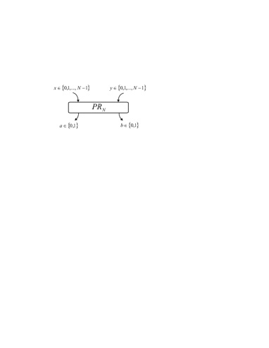
FIG. 1.: An N-inputs NLM: generalization of the two-inputs PR-box.

III Main result - Three settings

In this paper we present Bell-type inequalities allowing the use of some non-local resource. This means that all strategies satisfying such inequality can be simulated by local means (i.e. shared randomness, etc) together with some non-local resource — for example one NLM. In other words, any strategy violating such inequality would require a strictly larger amount of non-local resource than is allowed by the inequality. In the case of two settings, described in the previous Section, such inequalities cannot exist. This is because the most elementary non-local resource, the PR-box, suffices already to generate all the non-local vertices of the no-signaling polytope.

Therefore we switch to the next case, i.e. three settings (with two outputs) on each side. Here the situation becomes much more complicated but remains tractable. All facets of the local polytope have been listed [13]. No-signaling strategies are now living in a 15-dimensional space.

The local polytope. The local polytope has 64 vertices. Surprisingly it turns out that each of the $648$ non-trivial facets is equivalent to one of the two following Bell inequalities

CHSH $$\equiv \begin{array}[]{c|ccc}&-1&0&0\\ \hline\cr 0&0&0&0\\ -1&1&1&0\\ 0&1&-1&0\\ \end{array}\leq 0$$ (25)

$$I_{3322} \equiv \begin{array}[]{c|ccc}&-1&0&0\\ \hline\cr-2&1&1&1\\ -1&1&1&-1\\ 0&1&-1&0\\ \end{array}\leq 0$$ (30)

The CHSH inequality is still a facet of the local polytope. This is a general property of Bell inequalities, known as ”lifting” [18]: a facet Bell inequality, defined in a given configuration, remains a facet when the number of settings, outcomes or parties is augmented.

Quantum mechanics indeed violates the three-settings CHSH inequality. The second inequality, $I_{3322}$, is also violated by quantum mechanics. Furthermore this inequality is relevant, since it is violated by some quantum states which do not violate the CHSH inequality [13].

The no-signaling polytope. The local polytope has 72 CHSH-type facets. Above each of these facets lies a PR-box. This is clear since the CHSH inequality, while still being a facet of any local polytope with more settings, is a true two-inputs Bell inequality. Now it is interesting to see that above each $I_{3322}$ inequality (which is a true three-inputs Bell inequality) we find a no-signaling strategy which is more non-local than a PR-box. This strategy is represented by a three-inputs NLM, defined by the relation $[xy/2]=a+b(\textrm{mod 2})\,$, where $x,y\in\{0,1,2\}$ and $a,b\in\{0,1\}$. This machine will be refered to as $PR_{3}$. In probability space this new machine corresponds to the point

$$PR_{3} = \frac{1}{2}\times\begin{array}[]{c|ccc}&1&1&1\\ \hline\cr 1&1&1&1\\ 1&1&1&0\\ 1&1&0&1\\ \end{array}\,.$$ (35)

Note that $\langle I_{3322}|PR_{3}\rangle=1$, while $\langle I_{3322}|PR\rangle=0.5$ (see Fig. 2). Here we have used a scalar product-type notation $\langle I|S\rangle=z$, which means that testing inequality $I$ with strategy $S$ gives a value $z$. The machine $PR_{3}$ can be simply obtained from the inequality $I_{3322}$ using the Recipe mentioned at the end of the Section II. One needs two PR-boxes to simulate $PR_{3}$, as shown in Appendix A. $PR_{3}$ can also be rewritten in the elegant manner $x=y\,\Leftrightarrow a=b$, which corresponds to the probability point

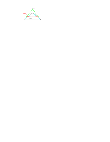
FIG. 2.: A facet $I_{3322}$ viewed in a simplified representation of the probability space. Above the facet, on the hyperplane $I_{3322}=0.5$, lie 28 strategies with a single PR. Above this hyperplane ($I_{3322}=1$) lie two strategies with a single $PR_{3}$. The local polytope is in black and the no-signaling in green. In blue is the polytope of all strategies using at most one PR; $M_{3322}$ is a facet of this polytope. The quantum set is in red. Note that some quantum states violate $M_{3322}$ (shaded area).

$$\frac{1}{2}\times\begin{array}[]{c|ccc}&1&1&1\\ \hline\cr 1&1&0&0\\ 1&0&1&0\\ 1&0&0&1\\ \end{array}\,.$$ (40)

The distribution (40) is indeed equivalent to (35) up to local symmetries: here both Alice and Bob flip their outputs for their first setting.

In a recent paper Jones and Masanes [19] gave a complete characterization of all the vertices of the no-signaling polytope for any number of settings and two outcomes — note that Barrett et al. studied the reversed case: two settings and any number of outcomes [16]. From their result it is clear that all vertices of the no-signaling polytope for three settings and two outputs can be constructed with a $PR_{3}$.

Numerically we find all the vertices of the no-signaling polytope. We proceed as follows. First we generate all strategies that use at most one $PR_{3}$. These are all the strategies where Alice and Bob can choose each of their three inputs in the set $\{0d,1d,0m,1m,2m,0mf,1mf,2mf\}$. Here $0d,1d$ means that they deterministically output the value $0$ or $1$; $0m,1m,2m$ means that they input $0,1,2$ in the machine $PR_{3}$; $0mf,1mf,2mf$ means that they input $0,1,2$ in $PR_{3}$ and flip the output of the machine. Second, we remove those strategies which are inside the local polytope by testing all the 648 Bell inequalities. Finally there are 1344 strategies left which are the non-local vertices of the (three-inputs two-outcomes) no-signaling polytope. We find four different classes of those vertices — given in Appendix B. A curious feature of those points is that each of them violates several inequalities of the local polytope. For example the strategy

$$PR = \frac{1}{2}\times\begin{array}[]{c|ccc}&1&1&0\\ \hline\cr 0&0&0&0\\ 1&1&1&0\\ 1&1&0&0\\ \end{array}\,$$ (45)

violates the CHSH inequality (25). But it clearly also violates eight $I_{3322}$-type inequalities, among which

$$\begin{array}[]{c|ccc}&-1&0&0\\ \hline\cr-2&1&1&1\\ -1&1&1&-1\\ 0&1&-1&0\\ \end{array}\leq 0\quad\begin{array}[]{c|ccc}&-1&0&-1\\ \hline\cr 0&-1&-1&1\\ -1&1&1&0\\ 0&1&-1&0\\ \end{array}\leq 0\,\,.$$ (54)

Formally this is clear, since each of these eight $I_{3322}$ inequalities (for example (54)) reduces to the CHSH inequality (25) once Alice’s third setting and Bob’s first setting are discarded. Fig. 3 gives some geometrical intuition of the situation.

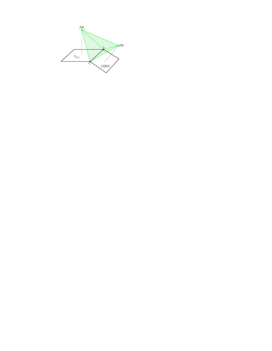
FIG. 3.: Simplified 3-dimensional view of a facet of the no-signaling polytope (green shaded surface). Among the extremal points of this facet are a PR-box strategy (45), a $PR_{3}$ (35) strategy, and a deterministic strategy $L_{0}=[0_{d},0_{d},0_{d};0_{d},0_{d},0_{d}]$. Behind this facet is another no-signaling facet which has a vertice $L_{1}=[1_{d},1_{d},1_{d};1_{d},1_{d},1_{d}]$. Indeed, $L_{0},L_{1}$ are extremal points of the local polytope. Note that PR and $PR_{3}$ are both above the CHSH and the $I_{3322}$ facets.

Inequality with a PR-box. We have just seen that, in the case of three settings on each side, there are two types of NLM, the PR-box and the $PR_{3}$, generating different types of non-local vertices of the no-signalling polytope. As mentioned, the $PR_{3}$ is a stronger non-local resource than the PR-box — it needs two PR-boxes to be simulated. Thus there is a new polytope, sandwiched between the local and the no-signaling polytopes. It is formed by all strategies that can be simulated using at most one PR-box (see Fig. 2). A facet of this polytope was recently found [11]. It corresponds to the inequality

$$M_{3322} \equiv \begin{array}[]{c|ccc}&-2&0&0\\ \hline\cr-2&1&1&1\\ -1&1&1&-1\\ 0&1&-1&0\\ \end{array}\leq 0\,$$ (59)

Although $M_{3322}$ is not violated by the maximally entangled state, it is violated by a family of non-maximally entangled states of two qubits [11]. Indeed the maximally entangled state does not violate this inequality, since its correlations can be simulated using a single PR-box [12]. Note that the structure of $M_{3322}$ is similar to $I_{3322}$, the only difference being the coefficient of Alice’s first marginal.

We prove now that $M_{3322}$ is a facet of the polytope of all strategies using at most one PR-box. This result will be extended to the case of N settings in the next section.

The proof consists of two parts: first we show that no strategy with a single use of a PR-box violates $M_{3322}$; then we show that there are (at least) $N(N+2)=15$ linearly independent strategies using at most one PR-box which saturate $M_{3322}$. Here we just sketch the idea of the proof, see Appendix C for details.

To prove the first part, we state a Lemma. Any no-signaling strategy S violating $M_{3322}$, also violates the two following inequalities

$$C_{1}\equiv\begin{array}[]{c|ccc}&-1&0&0\\ \hline\cr 0&0&0&0\\ -1&1&1&0\\ 0&1&-1&0\\ \end{array}\leq 0\quad C_{2}\equiv\begin{array}[]{c|ccc}&-1&0&0\\ \hline\cr-1&1&0&1\\ 0&1&0&-1\\ 0&0&0&0\\ \end{array}\leq 0\,\,.$$ (68)

The proof is straightforward. One needs only to note that, for no-signaling strategies, joint probabilities are smaller (or equal) than their respective marginals. Then by inverting the Lemma, we get the following proposition: if S does not violate both inequalities $C_{1}$ and $C_{2}$, then S does not violate $M_{3322}$. Finally it is obvious that with a single PR-box one can violate either $C_{1}$ or $C_{2}$, but not both at the same time.

For the second part of the proof, we find numerically eight local deterministic distributions which saturate $M_{3322}$. Then we find 57 other strategies with one PR-box saturating $M_{3322}$. Altogether these strategies form an hyperplane of dimension 14. This completes the proof that $M_{3322}$ is a facet of the polytope.

IV N settings

In this Section, the results of Section III are extended to the case of an arbitrary number of settings $N$. We use a family of Bell inequalities, known as $I_{NN22}$, which were proven to be facets of the local polytope [13]. These inequalities are generalization of the $I_{3322}$ seen before. For $N$ settings, the inequality reads

$$I_{NN22}\equiv\begin{array}[]{c|cccccc}&-1&0&0&\cdots 0&0\\ \hline\cr-(N-1)&1&1&1&\dots&1&1\\ -(N-2)&1&1&1&\cdots&1&-1\\ -(N-3)&1&1&1&\cdots&-1&0\\ \vdots&\vdots&&&&&\vdots\\ -1&1&1&-1&\cdots&0&0\\ 0&1&-1&0&\cdots&0&0\\ \end{array}\leq 0\,.$$ (76)

Using the Recipe of Section II, we construct a family of $N$-settings NLM

$$PR_{N}\equiv\frac{1}{2}\begin{array}[]{c|cccccc}&1&1&1&\cdots&1&1\\ \hline\cr 1&1&1&1&\dots&1&1\\ 1&1&1&1&\cdots&1&0\\ 1&1&1&1&\cdots&0&1\\ \vdots&\vdots&&&&&\vdots\\ 1&1&1&0&\cdots&1&1\\ 1&1&0&1&\cdots&1&1\\ \end{array}\,.$$ (84)

In order to simulate $PR_{N}$ one needs $N-1$ PR-boxes. This is easily shown using a straightforward generalization of Appendix A. The inequality

$$M_{(N+1)22}\equiv\begin{array}[]{c|ccccc}&-N&0&\cdots&0&0\\ \hline\cr-N&1&1&\dots&1&1\\ -(N-1)&1&1&\cdots&1&-1\\ -(N-2)&1&1&\cdots&-1&0\\ \vdots&\vdots&\vdots&&&\vdots\\ -1&1&1&\cdots&0&0\\ 0&1&-1&\cdots&0&0\\ \end{array}\leq 0$$ (92)

is an $(N+1)$-setting Bell inequality that cannot be violated by strategies which require a single use of $PR_{N}$, as proven in Appendix C. In (92) we have omitted a factor ($N+1$) in the name of the inequality for practical reasons. Again the structure of $M_{NN22}$ is similar to $I_{NN22}$, up to Alice’s first marginal: in order to get $M_{NN22}$ from $I_{NN22}$, one simply changes Alice’s first marginal to $-(N-1)$.

So finally we get the following nice construction. For any number of settings $N$ we have a Bell inequality $I_{NN22}$ and an $N$-input NLM ($PR_{N}$) which reaches the upper no-signaling bound of $I_{NN22}$. From there, we construct an $(N+1)$-setting inequality ($M_{(N+1)(N+1)22}$) which cannot be violated with one use of $PR_{N}$, i.e.

$$(I_{NN22},PR_{N})\quad\longrightarrow\quad(M_{(N+1)(N+1)22},PR_{N+1})$$ (93)

V Conclusion

To conclude, we review briefly the main results concerning polytopes and Bell inequalities with and without non-local resources. We focus on two-outcomes settings. Table I summarizes the situation. The oldest result is due to Fine, who showed that all (non-trivial) facets of the two-inputs two-outcomes local polytope are equivalent to the CHSH inequality [17]. Then Collins and Gisin completely characterized the case of three settings [13]. In particular they showed that there is a single new inequality ($I_{3322}$) which is inequivalent to CHSH. They also found a family of facet inequalities $I_{NN22}$ of the $N$ setting local polytope, but for $N>3$ it is not known if there are other inequalities. The vertices of the no-signaling polytope for two settings and any number of outcomes have been characterized by Barrett et al. [16], while Jones and Masanes studied the reversed case: an arbitrary number of settings with two outcomes [19].

Not much is known about inequalities allowing non-local resources. In 2003 Toner and Bacon found inequalities allowing one bit of communication for the case of two and three settings [20]. They showed that the correlations from measurements on any quantum state satisfy those inequalities. In the present paper we introduced a family of $N$ inputs NLMs ($\{PR_{N}\}_{N\geq 3}$), which are a generalization of the well-known PR-box. These NLMs can be derived from Bell inequalities in the same way than the PR-box is derived from the CHSH inequality. Then we presented a new family of inequalities ($\{M_{NN22}\}_{N\geq 3}$) allowing one use of $PR_{N}$.

For $N=3$, we get an inequality which cannot be violated with a single PR-box. This inequality, presented in a previous work [11], is however violated by some non-maximally entangled state of two qubits. Here we checked numerically that no states of two qubits violates $M_{4422}$ and $M_{5522}$, which suggests that these states could be simulated with two PR-boxes, or even a $PR_{3}$-box. However such model has still not been found.

We acknowledge support from the project QAP (IST-FET FP6-015848).

VI Appendix A

In this Appendix, we show how to construct a $PR_{3}$ with 2 PR-boxes.

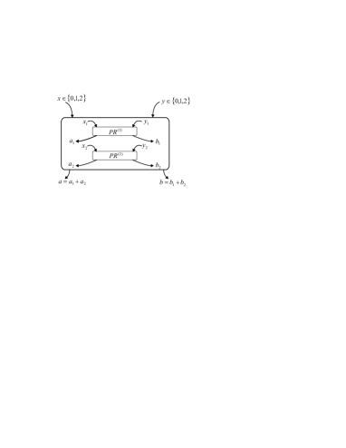
FIG. 4.: A $PR_{3}$ with two PR’s. The inputs of each PR, $x_{1,2}$ and $y_{1,2}$ are bits. For each ternary input $x$ ($y$), there is a combination of $x_{1,2}$ ($y_{1,2}$). Finally the output on each side is the sum (modulo 2) of the two binary outputs of the PR-boxes.

Alice and Bob each receive a trit. For each value of the trit they input one bit in each PR-box. The strategy is the following

$$\begin{array}[]{c|cc}x&x_{1}&x_{2}\\ \hline\cr 0&0&0\\ 1&0&1\\ 2&1&0\\ \end{array}\quad\quad\begin{array}[]{c|cc}y&y_{1}&y_{2}\\ \hline\cr 0&0&0\\ 1&1&0\\ 2&0&1\\ \end{array}$$ (102)

where $x,y$ denote the settings, and $x_{i},y_{i}$ are the binary inputs into PR-box number $i$. Finally, Alice and Bob output the sum (modulo 2) of both outputs of the PR-boxes. Intuitively the strategy works as follows. The first machine introduces an anti-correlation of the outputs for the pair of settings $x=1,y=2$. The second PR-box does the same for $x=2,y=1$. A nice way to show that this strategy works is by computing the parity of the outputs for each pair of settings. So we compute a parity matrix $P$ by multiplying Alice strategy by the transpose of Bob’s strategy

$$P=S_{A}S_{B}^{{\dagger}}=\left(\begin{array}[]{cc}0&0\\ 0&1\\ 1&0\\ \end{array}\right)\left(\begin{array}[]{ccc}0&1&0\\ 0&0&1\end{array}\right)=\left(\begin{array}[]{ccc}0&0&0\\ 0&0&1\\ 0&1&0\end{array}\right)\quad.$$ (111)

Note that matrix P has the same structure as the correlation terms of $I_{3322}$. So Alice and Bob’s outputs are identical when a 1 appears in the inequality and different when -1 is in the inequality.

This construction is easily generalized to $N$ settings. Since $I_{NN22}$ has $N-1$ correlation terms equal to -1, one simply uses a PR-box to anti-correlate the outcomes for each of those terms. Thus it can be shown that a $PR_{N}$ NLM is constructed with $N-1$ PR-boxes.

VII Appendix B

We find four classes of non-local vertices of the three-settings two-outcomes no-signaling polytope

$$S_{1} = \begin{array}[]{c|ccc}&x&x&x\\ \hline\cr x&x&x&x\\ x&x&x&0\\ x&x&0&x\\ \end{array}\quad S_{2}=\begin{array}[]{c|ccc}&x&x&0\\ \hline\cr 0&0&0&0\\ x&x&x&0\\ x&x&0&0\\ \end{array}$$ (120)

$$S_{3} = \begin{array}[]{c|ccc}&x&x&0\\ \hline\cr x&x&x&0\\ x&x&x&0\\ x&x&0&0\\ \end{array}\quad S_{4}=\begin{array}[]{c|ccc}&x&x&x\\ \hline\cr x&x&x&x\\ x&x&x&x\\ x&x&0&x\\ \end{array}$$ (129)

where $x=\frac{1}{2}$. Class $S_{1}$ corresponds to strategies with a $PR_{3}$. They violate maximally $I_{3322}$, i.e. up to $1$. Classes $S_{2}-S_{4}$ are strategies which can be obtained with a PR-box. In $S_{2}$, Alice and Bob have a deterministic output for one of their setting; in $S_{3}$, only Alice (or Bob) has a deterministic setting; in $S_{4}$, none outputs deterministic values.

There are 192 vertices in class 1, 288 in class 2, 576 in class 3, and 288 in class 4. All strategies in the same class violate the same number of CHSH inequalities and the same number of $I_{3322}$ inequalities. These numbers are summarized in the table below. For each class of vertices, the number of CHSH and $I_{3322}$ inequalities violated is given.

Class	CHSH	$I_{3322}$
$S_{1}$	6	18
$S_{2}$	1	8
$S_{3}$	2	12
$S_{4}$	4	24

VIII Appendix C

Here it is shown that inequality

$$M_{NN22}\equiv\begin{array}[]{c|cccccc}&-(N-1)&0&0&\cdots 0&&0\\ \hline\cr-(N-1)&1&1&1&\dots&1&1\\ -(N-2)&1&1&1&\cdots&1&-1\\ -(N-3)&1&1&1&\cdots&-1&0\\ \vdots&\vdots&&&&&\vdots\\ -1&1&1&-1&\cdots&0&0\\ 0&1&-1&0&\cdots&0&0\\ \end{array}\leq 0\,,$$ (137)

is a facet of the polytope containing all strategies that use (at most) one $PR_{N-1}$. The proof is in two parts. First we show that no strategy with a $PR_{N-1}$ can violate $M_{NN22}$. Then we show that the inequality is indeed a facet, i.e. we show that the strategies saturating the inequality ($M_{NN222}=0$) form a $(d-1)$-dimensional hyperplane, where $d=N(N+2)$ is the dimension of the probability space.

Part 1. We start with a Lemma.

Lemma 1. Let’s define the two inequalities

$$C^{N}_{1}\equiv\begin{array}[]{c|cccccc}&-(N-2)&0&0&\cdots 0&&0\\ \hline\cr 0&0&0&0&\dots&0&0\\ -(N-2)&1&1&1&\cdots&1&0\\ -(N-3)&1&1&1&\cdots&-1&0\\ \vdots&\vdots&&&&&\vdots\\ -1&1&1&-1&\cdots&0&0\\ 0&1&-1&0&\cdots&0&0\\ \end{array}\leq 0$$ (145)

$$C^{N}_{2}\equiv\begin{array}[]{c|cccccc}&-(N-2)&0&0&\cdots 0&&0\\ \hline\cr-(N-2)&1&0&1&\dots&1&1\\ -(N-3)&1&0&1&\cdots&1&-1\\ -(N-4)&1&0&1&\cdots&-1&0\\ \vdots&\vdots&&&&&\vdots\\ 0&1&0&-1&\cdots&0&0\\ 0&0&0&0&\cdots&0&0\\ \end{array}\leq 0\,.$$ (153)

Let S be a strategy with N settings for each of the two partners. S is in a probability space of dimension $N(N+2)$. If S violates inequality $M_{NN22}$, then S also violates both inequalities $C^{N}_{1}$ and $C^{N}_{2}$.

Proof. S violates $M_{NN22}$, i.e.

$$-(N-1)P(A_{0})-\sum^{N-2}_{k=0}(N-k-1)P(B_{k})+\sum^{N-1}_{k=0}P(A_{k}B_{0})$$ (154)

$$+\sum_{m=1}^{N-1}\bigg{[}\bigg{(}\sum^{N-m-1}_{k=0}P(A_{k}B_{m})\bigg{)}-P(A_{N-m}B_{m})\bigg{]}>0$$ (155)

According to the no-signaling condition, we have

$$P(A_{0})\geq P(A_{0}B_{0})$$ (156)

$$(N-1)P(B_{0})\geq\sum^{N-1}_{k=1}P(A_{k}B_{0})$$ (157)

$$P(A_{N-1}B_{1})\geq 0$$ (158)

Inserting these relations into (154) we get,

$$-(N-2)P(A_{0})-\sum^{N-2}_{k=1}(N-k-1)P(B_{k})+\sum^{N-2}_{k=0}P(A_{k}B_{1})$$

$$+\sum_{m=2}^{N-1}\bigg{[}\bigg{(}\sum^{N-m-1}_{k=0}P(A_{k}B_{m})\bigg{)}-P(A_{N-m}B_{m})\bigg{]}>0$$

which means S violates inequality $C_{1}^{N}$.

Again from to the no-signaling condition, we have

$$P(A_{0})\geq P(A_{0}B_{N-1})$$ (159)

$$P(B_{j})\geq P(A_{1}B_{j})\quad\quad\forall j\in\{0,N-1\}$$ (160)

$$P(A_{1}B_{N-1})\geq 0$$ (161)

which inserted into (154) gives

$$-(N-2)P(A_{0})-\sum^{N-3}_{k=0}(N-k-2)P(B_{k})$$

$$+\sum^{N-2}_{k=0}P(A_{0}B_{k})+\sum^{N-1}_{k=2}P(A_{k}B_{0})$$

$$+\sum_{m=1}^{N-3}\bigg{[}\bigg{(}\sum^{N-m-1}_{k=2}P(A_{k}B_{m})\bigg{)}-P(A_{N-m}B_{m})\bigg{]}$$

$$-P(A_{2}B_{N-2})>0$$

which means S violates inequality $C_{2}^{N}$.

This completes the first part of the proof.

Part 2. Now we have to show that there are at least $N(N+2)$ strategies using at most one NLM $P_{N-1}$ on the hyperplane defined by

$$M_{NN22}=0\,.$$ (162)

Let’s consider only deterministic strategies. We show that there are $2^{N}$ of them on the $M_{NN22}$ facet.

First we note that there are eight local strategies on the $M_{3322}$ facet.

$$\begin{array}[]{c|ccc}&0&1&1\\ \hline\cr 1&0&1&1\\ 0&0&0&0\\ 0&0&0&0\\ \end{array}\quad\begin{array}[]{c|ccc}&0&1&1\\ \hline\cr 0&0&0&0\\ 0&0&0&0\\ 0&0&0&0\\ \end{array}\quad\begin{array}[]{c|ccc}&0&1&0\\ \hline\cr 0&0&0&0\\ 1&0&1&0\\ 0&0&0&0\\ \end{array}\quad\begin{array}[]{c|ccc}&0&1&0\\ \hline\cr 0&0&0&0\\ 0&0&0&0\\ 0&0&0&0\\ \end{array}$$ (179)

$$\begin{array}[]{c|ccc}&0&0&1\\ \hline\cr 0&0&0&0\\ 0&0&0&0\\ 1&0&0&1\\ \end{array}\quad\begin{array}[]{c|ccc}&0&0&1\\ \hline\cr 0&0&0&0\\ 0&0&0&0\\ 0&0&0&0\\ \end{array}\quad\begin{array}[]{c|ccc}&0&0&0\\ \hline\cr 0&0&0&0\\ 0&0&0&0\\ 1&0&0&0\\ \end{array}\quad\begin{array}[]{c|ccc}&0&0&0\\ \hline\cr 0&0&0&0\\ 0&0&0&0\\ 0&0&0&0\\ \end{array}$$ (196)

Obviously the marginals fix entirely a deterministic strategy. Then it is clear that if a three settings strategy

$$S=\begin{array}[]{c|ccc}&A_{0}&A_{1}&A_{2}\\ \hline\cr B_{0}&&&\\ B_{1}&&\cdots&\\ B_{2}&&&\\ \end{array}$$ (201)

is on the facet $M_{3322}$, then both (four settings) strategies

$$S^{\prime}=\begin{array}[]{c|cccc}&A_{0}&A_{1}&A_{2}&0\\ \hline\cr 0&0&0&0&0\\ B_{0}&&&&0\\ B_{1}&&\cdots&&0\\ B_{2}&&&&0\\ \end{array}$$ (207)

$$S^{\prime\prime}=\begin{array}[]{c|cccc}&A_{0}&A_{1}&A_{2}&1\\ \hline\cr B_{0}&&&&\beta_{0}\\ B_{1}&&\cdots&&\beta_{1}\\ B_{2}&&&&\beta_{2}\\ 0&0&0&0&0\\ \end{array}$$ (213)

are on the facet $M_{4422}$. The notation $\beta_{j}$ for some correlation coefficients means that their value depends on Bob’s marginal. Indeed all these strategies are extremal since they are deterministic.

Then the argument is extended to the next case: for each of the 16 strategies (constructed above) which lie on $M_{4422}$, there are two strategies on $M_{5522}$. Thus there are $2^{N}$ deterministic strategies on $M_{NN22}$. Note that $2^{N}>N(N+2)$ for $N\geq 6$. In this case the number of local strategies on the hyperplane $M_{NN22}=0$ is larger than the dimension of the probability space. This shows that $M_{NN22}$ is a facet of the polytope of all strategies using at most one $PR_{N-1}$. For the case of $N=4$ and $N=5$, we checked numerically that all strategies using at most one $PR_{N-1}$ form a subspace of dimension $d-1$, where $d=N(N+2)$ is the dimension of the probability space.

Resource	$N=2$	$N=3$	$N\geq 4$
lhv	CHSH   [17]	CHSH+$I_{3322}\,\cite[cite]{[\@@bibref{Number}{dan}{}{}]}$	CHSH+$\{I_{NN22}\}_{N\geq 3}$ +??   [13]
PR-box	—	$M_{3322}$   [11]	$M_{3322}+$??
1 bit	—	[3]	??
$PR_{N-1}$	—	[11]	$M_{NN22}$   (this paper)   +??
no-signaling	PR [16]	$PR+PR_{3}$   [19]	$PR+\{PR_{N}\}_{N\geq 3}$ [19]

TABLE I.: Main results about Bell inequalities with and without non-local resources. We consider only the case of binary outcomes. $N$ is the number of settings. The last line represents the vertices of the no-signaling polytope. The first column is almost empty since, for two settings, any no-signaling correlation can be generated with a PR-box. The question marks mean that it is not known if there are more of these inequalities. For $N=3$, we are quite confident that $M_{3322}$ is the only inequality for one use of a PR-box, though we could not prove it rigorously.

REFERENCES

- [1] J.S. Bell, Physics 1 195 (1964)
- [2] A. Aspect, Nature 398 189 (1999)
- [3] B.F. Toner and D. Bacon, Phys. Rev. Lett. 91 187904 (2003)
- [4] S. Popescu and D. Rohrlich, Found. Phys. 24 379 (1994)
- [5] B.S. Tsirelson, Hadronic J. Supplement 8, 329 (1993)
- [6] W. van Dam, quant-ph/0501159
- [7] G. Brassard, Found. Phys 33 1593 (2003)
- [8] J. Barrett, L. Hardy, A. Kent, Phys. Rev. Lett. 95, 010503 (2005) ; A.Acin, L. Masanes, N. Gisin, quant-ph/0510094
- [9] J. Barrett, S. Pironio, Phys. Rev. Lett. 95, 140401 (2005)
- [10] In order to construct a no-signaling strategy with classical communication, one has to cleverly hide the communication, to avoid signaling. See for example: J. Degorre, S. Laplante, J. Roland, Phys. Rev. A 72, 062314 (2005); or also [11].
- [11] N. Brunner, N. Gisin, V. Scarani, New J. Phys. 7, 88 (2005)
- [12] N. Cerf, N. Gisin, S. Massar, S. Popescu, quant-ph/0410027
- [13] D. Collins and N. Gisin, J. Phys. A: Math. Gen. 37 1775 (2004)
- [14] J.F. Clauser, M.A. Horne, A. Shimony, R.A. Holt, Phys. Rev. Lett. 23, 880 (1969)
- [15] I. Pitowski, Quantum Probability, Quantum Logic, Lecture Notes in Physics 321 (Springer Verlag, Heidelberg, 1989)
- [16] J. Barrett, N. Linden, S. Massar, S. Pironio, S. Popescu and D. Roberts, Phys Rev. A 71, 022101 (2005)
- [17] A. Fine, Phys. Rev. Lett. 48 291-295 (1982)
- [18] S. Pironio, J. Math. Phys. 46, 062112 (2005)
- [19] N. Jones and L. Masanes, Phys. Rev. A 72, 052312 (2005)
- [20] D. Bacon and B.F. Toner, Phys. Rev. Lett. 90, 157904 (2003)