Bloch-Zener oscillations

Abstract

It is well known that a particle in a periodic potential with an additional constant force performs Bloch oscillations. Modulating every second period of the potential, the original Bloch band splits into two subbands. The dynamics of quantum particles shows a coherent superposition of Bloch oscillations and Zener tunneling between the subbands, a Bloch-Zener oscillation. Such a system is modelled by a tight-binding Hamiltonian, a system of two minibands with an easily controllable gap. The dynamics of the system is investigated by using an algebraic ansatz leading to a differential equation of Whittaker-Hill type. It is shown that the parameters of the system can be tuned to generate a periodic reconstruction of the wave packet and thus of the occupation probability. As an application, the construction of a matter wave beam splitter and a Mach-Zehnder interferometer is briefly discussed.

1 Introduction

Since the beginning of quantum mechanics, the dynamics of a particle in a periodic potential is a subject of fundamental interest. The eigenenergies of such a system form the famous Bloch bands, where the eigenstates are delocalized states and lead to transport [1]. If an additional static field $F$ is introduced, the eigenstates become localized. Counterintuitively, transport is dramatically reduced and an oscillatory motion is found, the famous Bloch oscillation. During the last decade these Bloch oscillations have been experimentally observed for various systems: electrons in semiconductor superlattices [2], cold atoms in optical lattices [3], light pulses in photonic crystals [4, 5] and even mechanical systems may Bloch-oscillate [6].

If the external field is strong enough, tunneling between Bloch bands becomes possible, as already discussed by Zener long ago [7]. In general, successive Zener tunneling to even higher bands will lead to decay as the bandgaps usually decrease with increasing energy. This decay can be observed as pulsed output for a Bose-Einstein condensate in an optical lattice [8], for electrons in semiconductor superlattices [9] or for light in waveguide arrays [10]. In this case a description in terms of Wannier–Stark resonances is more suited than the common Bloch band picture [11].

In order to study and exploit the interplay between Bloch oscillations and Zener tunneling, a system of at least two bands is needed, which are well separated from all other bands. This is achieved by introducing another weak potential with a doubled period length. Due to this pertubation, the ground band splits into two minibands and Zener tunneling between the minibands must be taken into account.

In this paper we discuss the dynamics in such a period-doubled potential within the tight-binding approximation. We assume that the ground state energies of the potential wells are alternately increased or decreased by the additional potential. The Hamiltonian then reads

$$\hskip 8.53581pt\hat{H}=-\frac{\Delta}{4}\sum\limits_{n=-\infty}\limits^{\infty}(|n\rangle\langle n+1|+|n\rangle\langle n-1|)+\frac{\delta}{2}\sum\limits_{n=-\infty}\limits^{\infty}(-1)^{n}|n\rangle\langle n|+Fd\sum\limits_{n=-\infty}\limits^{\infty}n|n\rangle\langle n|\,,$$ (1)

where $|n\rangle$ is the Wannier state localized in the $n$th potential well. Furthermore, $\Delta$ denotes the width of the unperturbed band ($\delta=0$), $\delta$ gives the gap between the two minibands at the edge of the Brillouin zone and $F$ is the external force. For $\delta=0$ this Hamiltonian reduces to the celebrated single-band tight-binding model, which has been studied in great detail (see [12] for a recent review). The period-doubled tight-binding model was introduced for the field-free case $F=0$ already in 1988 [13]. First pertubation theoretical results with an external field can be found in [14, 15]. Numerical results for an analogous two-miniband system in two spatial dimensions were reported in [16, 17].

This paper is organized as follows: First of all we repeat some results for the field free system $F=0$. The spectral properties for the case $F\neq 0$ are discussed in section 3, and the dynamics is analyzed in detail in section 4. We present an algebraic ansatz for the time evolution operator and analyze the time evolution by general arguments. The interesting case of periodic, i.e. reconstructing, Bloch-Zener oscillations and thus reconstructing occupation probabilities is analyzed in detail. These theoretical considerations are illustrated by some numerical results. As an application of Bloch-Zener oscillations, a beam splitting mechanism for matter waves is described and simulated numerically. The possibility of constructing a Mach-Zehnder interferometer based on Bloch-Zener oscillations is briefly discussed.

2 Bloch bands in the field-free case

First of all we discuss the spectrum of the period-doubled Hamiltonian (1) for the field-free case $F=0$, i.e. Bloch bands and Bloch waves. A straightforward calculation yields the dispersion relation

$$E_{\beta,\kappa}=\frac{\gamma}{2}(-1)^{\beta+1}\sqrt{\delta^{2}+\Delta^{2}\cos^{2}(\kappa d)},$$ (2)

with the miniband index $\beta=0,1$ and $\gamma={\rm sgn}(\delta)$, which is illustrated in figure 1. For $\delta\neq 0$, the Bloch band splits into two minibands with band gap $\delta$.

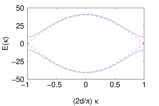
Figure 1: Dispersion relation of the double-periodic system in the reduced Brillouin zone for $\Delta=80$. The Bloch bands for $\delta=0$ (dashed curve) split into two minibands with gap $\delta$ (solid lines for $\delta=18$).

The Bloch waves $|\chi_{\beta,\kappa}\rangle$ of both bands are given by

$$|\chi_{0,\kappa}\rangle =\frac{1}{\sqrt{N_{\kappa}}}\sum\limits_{n=-\infty}\limits^{\infty}u_{\kappa}\,\rme^{\rmi(2n+1)\kappa d}|2n\rangle+\frac{1}{\sqrt{N_{\kappa}}}\sum\limits_{n=-\infty}\limits^{\infty}v_{\kappa}\,\rme^{\rmi(2n+2)\kappa d}|2n+1\rangle$$ (3)

$$|\chi_{1,\kappa}\rangle =\frac{1}{\sqrt{N_{\kappa}}}\sum\limits_{n=-\infty}\limits^{\infty}v_{\kappa}\,\rme^{\rmi(2n)\kappa d}|2n\rangle-\frac{1}{\sqrt{N_{\kappa}}}\sum\limits_{n=-\infty}\limits^{\infty}u_{\kappa}\,\rme^{\rmi(2n+1)\kappa d}|2n+1\rangle$$ (4)

with normalization constant $N_{\kappa}=\pi(u_{\kappa}^{2}+v_{\kappa}^{2})/d$ and coefficents

$$u_{\kappa}=\Delta\cos(\kappa d)\quad\mbox{and}\quad v_{\kappa}=\delta+\gamma\sqrt{\delta^{2}+\Delta^{2}\cos^{2}(\kappa d)}.$$ (5)

In the Bloch basis, the time independent Schrödinger equation with Hamiltonian (1) reads

$$E\langle\chi_{0,\kappa}|\Psi\rangle = E_{0,\kappa}\langle\chi_{0,\kappa}|\Psi\rangle+\rmi F\frac{\partial}{\partial\kappa}\langle\chi_{0,\kappa}|\Psi\rangle-Fd\langle\chi_{0,\kappa}|\Psi\rangle-M_{\kappa}\langle\chi_{1,\kappa}|\Psi\rangle\,$$ (6)

$$E\langle\chi_{1,\kappa}|\Psi\rangle = E_{1,\kappa}\langle\chi_{1,\kappa}|\Psi\rangle+\rmi F\frac{\partial}{\partial\kappa}\langle\chi_{1,\kappa}|\Psi\rangle+M_{\kappa}\langle\chi_{0,\kappa}|\Psi\rangle\,,$$ (7)

where the coupling of the two bands is given by the transition matrix element

$$\langle\chi_{1,\kappa^{\prime}}|\hat{H}_{ZB}|\chi_{0,\kappa}\rangle=M_{\kappa}\delta_{\frac{\pi}{d}}(\kappa-\kappa^{\prime})$$ (8)

with the reduced matrix element

$$M_{\kappa} = \rmi F\frac{\left(\frac{\partial}{\partial\kappa}u_{\kappa}\right)v_{\kappa}-\left(\frac{\partial}{\partial\kappa}v_{\kappa}\right)u_{\kappa}}{u_{\kappa}^{2}+v_{\kappa}^{2}}\,\rme^{\rmi\kappa d}=-\,\frac{\rmi Fd\Delta\delta\sin(\kappa d)\,\rme^{\rmi\kappa d}}{2\delta^{2}+2\Delta^{2}\cos^{2}(\kappa d)}\,$$ (9)

(cf. [14]). The modulus of $M_{\kappa}$ is shown in figure 2.

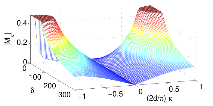
Figure 2: Absolute value of the reduced transition matrix element $|M_{\kappa}|$ for $\Delta=80$ and $dF=1$. The range $|M_{\kappa}|>0.5$ has been cut off to increase the visibility.

Obviously, the band transitions mainly take place at the edge of the Brillouin zone and, because of the delta-function in (8), only direct interband transitions are possible.

3 Spectral properties

We now discuss the spectrum of the two-miniband Hamiltonian (1) with an external field. The spectrum of the single-band Wannier-Stark Hamiltonian ($\delta=0$) consists of a ladder of equally spaced eigenvalues – the Wannier-Stark ladder. Note that beyond the single-band tight-binding approximation these eigenstates become resonances embedded into a continuum (see [11] for a review). In the case of two minibands, $\delta\neq 0$, the spectrum consists of two ladders with an offset in between, as will be shown below. Furthermore the dependence of the offset on the system parameters will be discussed in detail. Certain aspects of the spectrum were previously discussed in [14].

To keep the notation simple, we introduce the translation operator

$$\hat{T}_{m}=\sum\limits_{n=-\infty}\limits^{\infty}|n-m\rangle\langle n|\,$$ (10)

and an operator $\hat{G}$ that causes the inversion of the sign of $\delta$ in all following terms. They fulfil the following commutation relations

$$\left[\hat{T}_{m},\hat{H}\right] = \frac{\delta}{2}\sum\limits_{n=-\infty}\limits^{\infty}(-1)^{n}\left[1-(-1)^{m}\right]|n-m\rangle\langle n|$$ (11)

$$\quad+Fd\sum\limits_{n=-\infty}\limits^{\infty}m|n-m\rangle\langle n|\,,$$

$$\left[\hat{G},\hat{H}\right] = -\delta\sum\limits_{n=-\infty}\limits^{\infty}(-1)^{n}|n\rangle\langle n|\,\hat{G}\quad\mbox{and}\quad\left[\hat{T}_{m},\hat{G}\right]=0\,.$$ (12)

An eigenvector $|\Psi\rangle$ of $\hat{H}$ with the eigenvalue $E(\delta,\Delta,Fd)$,

$$\hat{H}|\Psi\rangle=E(\delta,\Delta,Fd)|\Psi\rangle\,,$$ (13)

satisfies

$$\hat{H}\left\{\hat{T}_{2l}|\Psi\rangle\right\} = \left\{E(\delta,\Delta,Fd)-2ldF\right\}\left\{\hat{T}_{2l}|\Psi\rangle\right\}\,,$$ (14)

$$\hat{H}\left\{\hat{T}_{2l+1}\hat{G}|\Psi\rangle\right\} = \left\{E(-\delta,\Delta,Fd)-(2l+1)Fd\right\}\left\{\hat{T}_{2l+1}\hat{G}|\Psi\rangle\right\}\,.$$ (15)

Thus the application of the operators $\hat{T}_{2l}$ resp. $\hat{T}_{2l+1}\hat{G}$ to the eigenvector $|\Psi\rangle$ yields two ladders of eigenvectors

$$\hat{H}|\Psi_{\alpha,n}\rangle=E_{\alpha,n}|\Psi_{\alpha,n}\rangle\quad\mbox{with}\quad\alpha=0,1$$ (16)

defined by

$$|\Psi_{0,n}\rangle=\hat{T}_{-2n}|\Psi\rangle\quad\mbox{and}\quad|\Psi_{1,n}\rangle=\hat{G}\hat{T}_{-(2n+1)}|\Psi\rangle$$ (17)

with equidistant eigenenergies

$$E_{0,n} = E(\delta,\Delta,Fd)+2ndF\,,$$ (18)

$$E_{1,n} = E(-\delta,\Delta,Fd)+(2n+1)dF\,.$$ (19)

Thus the spectrum of the Hamiltonian (1) consists of two energy ladders with equal spacings and an offset given by $E(\delta,\Delta,Fd)$. Furthermore it can be shown that there are not more than two different energy ladders (see appendix). The eigenvectors $|\Psi_{\alpha,n}\rangle$ are displaced by $2n$ lattice periods with respect to $|\Psi_{\alpha,0}\rangle$, where $\alpha$ labels the two ladders.

The dependence of $E(\delta,\Delta,Fd)$ on the system parameters $\delta$, $\Delta$ and $Fd$ shows several interesting symmetries. In the case $\delta=0$ it is well known that for all values of $\Delta$ and $Fd$ we can choose $E(0,\Delta,Fd)=0$ [12]. In the case $\delta\neq 0$ it can be shown that $E(-\delta,\Delta,Fd)=-E(\delta,\Delta,Fd)$ holds, as well as $E(\delta,-\Delta,Fd)=E(\delta,\Delta,Fd)$. The proofs of these relations are quite similar and only one of them is given here. We consider the operator $\hat{X}$ defined by

$$\hat{X}=\sum\limits_{n=-\infty}\limits^{\infty}|-n\rangle\langle n|\,(-1)^{n}\,,$$ (20)

which fulfils the relation

$$\hat{X}\hat{H}(\delta,\Delta,Fd)=-\hat{H}(-\delta,\Delta,Fd)\hat{X}.$$ (21)

Applying $-\hat{X}$ to equation (16) yields

$$-E_{\alpha,n}(\delta,\Delta,Fd)\left\{\hat{X}|\Psi_{\alpha,n}\rangle\right\} = \hat{H}(-\delta,\Delta,Fd)\left\{\hat{X}|\Psi_{\alpha,n}\rangle\right\}$$ (22)

$$=: E_{\alpha^{\prime},n^{\prime}}(-\delta,\Delta,Fd)\left\{\hat{X}|\Psi_{\alpha,n}\rangle\right\}.$$

This means that the whole spectrum is antisymmetric by means of

$$-E_{\alpha,n}(\delta,\Delta,Fd)=E_{\alpha^{\prime},n^{\prime}}(-\delta,\Delta,Fd)\,.$$ (23)

To simplify the following argumentation, we consider without loss of generality the whole spectrum $\mathcal{S}$ modulo $2dF$. Thus we get

$$\mathcal{S}=\{E(\delta,\Delta,Fd),E(-\delta,\Delta,Fd)+dF\}_{{\rm mod}\,2dF}\,.$$ (24)

For $-\delta$ the spectrum therefore reads

$$\mathcal{S}=\{E(-\delta,\Delta,Fd),E(\delta,\Delta,Fd)+dF\}_{{\rm mod}\,2dF}\,.$$ (25)

By equation (23) this must be equal to

$$\mathcal{S} = \{-E(\delta,\Delta,Fd),-E(-\delta,\Delta,Fd)-dF\}_{{\rm mod}\,2dF}$$ (26)

$$= \{-E(\delta,\Delta,Fd),-E(-\delta,\Delta,Fd)+dF\}_{{\rm mod}\,2dF}\,.$$

From the equivalence of the equations (25) and (26) it follows that

$$E(-\delta,\Delta,Fd)=-E(\delta,\Delta,Fd)\,.$$ (27)

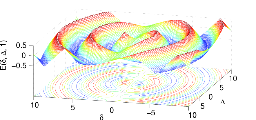
Figure 3: Alternating energy shift $E(\delta,\Delta,1)$ versus $\delta$ and $\Delta$ for $Fd=1$.

Numerical results for the energy offset $E(\delta,\Delta,1)$ and the energy ladders $E_{\alpha,n}(\delta,\Delta,1)$ are shown in figure 3 and figure 4. In all examples we consider only the case $Fd=1$, as all other cases can be reduced to it by a simple scaling

$$E_{\alpha,n}(\delta,\Delta,Fd)=dFE_{\alpha,n}\left(\textstyle\frac{\delta}{Fd}\displaystyle,\textstyle\frac{\Delta}{Fd},1\right)\displaystyle\,,$$ (28)

which directly follows from a rescaling of the Hamiltonian $\hat{H}$ by $Fd$.

In certain limits, one can easily derive some analytic approximations for the ladder offset $E(\delta,\Delta,Fd)$:

1. For $\delta\gg\Delta$ the two minibands are well separated energetically, so that their coupling can be neglected. Hence one sets $M_{\kappa}\approx 0$ in the equations (6) and (7). The energy shift is then given by

   $$E(\delta,\Delta,Fd) = \frac{\gamma}{\pi}\sqrt{\delta^{2}+\Delta^{2}}\,I\left(\textstyle\frac{\pi}{2}\displaystyle,\textstyle\sqrt{\frac{\Delta^{2}}{\delta^{2}+\Delta^{2}}}\displaystyle\right)$$ (29)

   $$= \frac{\gamma}{\pi}\int_{0}^{\pi/2}\sqrt{\delta^{2}+\Delta^{2}\cos^{2}y}\,\rmd y\,$$ (30)

   (compare [14]) with $\gamma={\rm sgn}(\delta)$. Here, $I$ denotes the incomplete elliptic integral of the second kind [18]. This approximation is compared to the numerical results in figure 4.

2. For small $\delta$ perturbation theory can be done, which yields

   $$E(\delta,\Delta,Fd)=\frac{\delta}{2}J_{0}\left(\textstyle\frac{\Delta}{Fd}\displaystyle\right)\,,$$ (31)

   where $J_{0}$ denotes the ordinary Bessel function.

The zeros of $E(\delta,0,1)$ are $\delta=0,\pm 2,\pm 4,\ldots$ (see figure 3), whereas the zeros of $E(\delta,\Delta,1)$ for very small $\delta$ are given by the zeros of $J_{0}(\Delta)$ (see equation (31)) which are $\Delta\approx n\pi$ for large $\Delta$. These relations indicate that the characteristic structure of the energy shift looks similar for large $\Delta$ and large $\delta$. In figure 4 one clearly sees the asymmetry of $E(\delta,\Delta,1)$ with respect to $\delta$. Avoided crossings appear in the typical case of $\Delta\neq 0$.

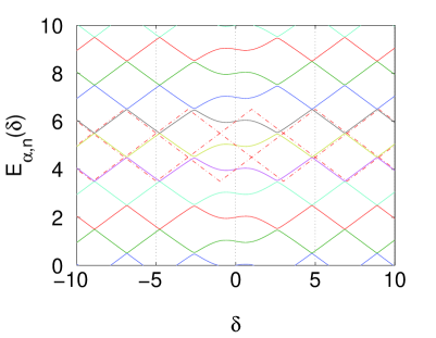
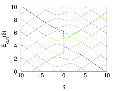
Figure 4: Spectrum $E_{\alpha,n}(\delta)$ of the Hamiltonian (1) for $Fd=1$ (solid lines). The left-hand side shows the case $\Delta=2$, where $\Delta=0$ is given as reference (dashed line). Note the avoided crossings of the energy levels. The right-hand side shows the spectrum for $\Delta=4$. Here two rungs of different energy ladders calculated with the approximation $M_{\kappa}\approx 0$ (dashed lines, cf. equation (30)) are shown for comparison.

4 Dynamics

4.1 An algebraic ansatz for the time evolution operator

In this section we derive some general results for the time evolution operator $\hat{U}$. The single-band system $\delta=0$ can be treated conveniently within a Lie-algebraic approach [19]. To simplify notation, we rewrite the Hamiltonian (1) using the operators

$$\hat{N} = \sum\limits_{n=-\infty}\limits^{\infty}n|n\rangle\langle n|\,,\quad\hat{L}=\sum\limits_{n=-\infty}\limits^{\infty}(-1)^{n}|n\rangle\langle n|=(-1)^{\hat{N}}\,,$$ (32)

$$\hat{K} = \sum\limits_{n=-\infty}\limits^{\infty}|n-1\rangle\langle n|\quad\mbox{and}\quad\hat{K}^{\dagger}=\sum\limits_{n=-\infty}\limits^{\infty}|n+1\rangle\langle n|\,.$$ (33)

These operators fulfil the commutator relations

$$\left[\hat{K},\hat{N}\right]=\hat{K}\,,\quad\quad\left[\hat{K}^{\dagger}\,,\hat{N}\right]=-\hat{K}^{\dagger}\,,\quad\quad\left[\hat{K}^{\dagger},\hat{K}\right]=0$$ (34)

and

$$\left[\hat{L},\hat{N}\right]=0\,,\quad\quad\left[\hat{K}^{\dagger}\,,\hat{L}\right]=2\hat{K}^{\dagger}\hat{L}\,,\quad\quad\left[\hat{K},\hat{L}\right]=2\hat{K}\hat{L}\,.$$ (35)

From the commutator relations of $\hat{K}^{\dagger}$, $\hat{K}$ and $\hat{L}$ one concludes that for any function $\hat{f}$ of the shift operators alone, one has

$$\hat{f}(\hat{K},\hat{K}^{\dagger})\hat{L}=\hat{L}\hat{f}(-\hat{K},-\hat{K}^{\dagger})\,.$$ (36)

The Schrödinger equation for the time evolution operator $\hat{U}$ then reads

$$\rmi\hbar\frac{\partial}{\partial t}\hat{U}=\left[-\frac{\Delta}{4}\left(\hat{K}+\hat{K}^{\dagger}\right)+\frac{\delta}{2}\hat{L}+Fd\hat{N}\right]\hat{U}\,.$$ (37)

In analogy to the single-band system [19] we make the ansatz

$$\hat{U}=\rme^{-\rmi C(t)\hat{N}}\left(\hat{A}(\hat{K},\hat{K}^{\dagger},t)+\hat{L}\hat{B}(\hat{K},\hat{K}^{\dagger},t)\right)$$ (38)

where $C(t)$, $\hat{A}(\hat{K},\hat{K}^{\dagger},t)$ and $\hat{B}(\hat{K},\hat{K}^{\dagger},t)$ are yet unknown functions or operators. To abbreviate the notation we do not write the arguments of the operator valued functions $\hat{A}(t)$ and $\hat{B}(t)$ in the following explicitly. Substituting equation (38) into (37) leads to

$$\hbar\,\dot{C}(t)\hat{N}\rme^{-\rmi C(t)\hat{N}}\left(\hat{A}\left(t\right)+\hat{L}\hat{B}\left(t\right)\right)+\rmi\hbar\,\rme^{-\rmi C(t)\hat{N}}\left(\dot{\hat{A}}\left(t\right)+\hat{L}\dot{\hat{B}}\left(t\right)\right)$$

$$\quad=Fd\hat{N}\rme^{-\rmi C(t)\hat{N}}\left(\hat{A}\left(t\right)+\hat{L}\hat{B}\left(t\right)\right)-\frac{\Delta}{4}\hat{K}\rme^{-\rmi C(t)\hat{N}}\left(\hat{A}\left(t\right)+\hat{L}\hat{B}\left(t\right)\right)$$

$$\quad-\frac{\Delta}{4}\hat{K}^{\dagger}\rme^{-\rmi C(t)\hat{N}}\left(\hat{A}\left(t\right)+\hat{L}\hat{B}\left(t\right)\right)+\frac{\delta}{2}\hat{L}\,\rme^{-\rmi C(t)\hat{N}}\left(\hat{A}\left(t\right)+\hat{L}\hat{B}\left(t\right)\right).$$ (39)

Here and in the following, the dot marks the derivative with respect to the time $t$. The first term of the left and the right side of equation (39) cancel each other if

$$\hbar\,\dot{C}(t)=Fd\quad\Longrightarrow\quad C(t)=\frac{d}{\hbar}\int\limits_{0}^{t}F(\tau)\,\rmd\tau.$$ (40)

The remaining terms in equation (39) can be simplified by multiplying with $\rme^{\rmi C(t)\hat{N}}$ from the left and using the relations

$$\rme^{\rmi C(t)\hat{N}}\hat{K}\rme^{-\rmi C(t)\hat{N}} = \rme^{-\rmi C(t)}\hat{K}\,,$$ (41)

$$\rme^{\rmi C(t)\hat{N}}\hat{K}^{\dagger}\rme^{-\rmi C(t)\hat{N}} = \rme^{\rmi C(t)}\hat{K}^{\dagger}\,,$$ (42)

which follow from the Baker-Hausdorff formula

$$\hskip 19.91692pt\rme^{z\hat{Y}}\,\hat{X}\rme^{-z\hat{Y}}=\hat{X}+z\left[\hat{Y},\hat{X}\right]+\frac{z^{2}}{2!}\left[\hat{Y},\left[\hat{Y},\hat{X}\right]\right]+\frac{z^{3}}{3!}\left[\hat{Y},\left[\hat{Y},\left[\hat{Y},\hat{X}\right]\right]\right]+\ldots.$$ (43)

Since $\hat{L}$ and $\hat{N}$ commute and $\hat{L}\hat{L}=\mathbb{1}$, one finally arrives at

$$\hat{L}\left(\rmi\hbar\dot{\hat{B}}\left(t\right)-\frac{\Delta}{4}\rme^{-\rmi C(t)}\hat{K}\hat{B}\left(t\right)-\frac{\Delta}{4}\rme^{\rmi C(t)}\hat{K}^{\dagger}\hat{B}\left(t\right)-\frac{\delta}{2}\hat{A}\left(t\right)\right)$$

$$\quad=-\left(\rmi\hbar\dot{\hat{A}}\left(t\right)+\frac{\Delta}{4}\rme^{-\rmi C(t)}\hat{K}\hat{A}\left(t\right)+\frac{\Delta}{4}\rme^{\rmi C(t)}\hat{K}^{\dagger}\hat{A}\left(t\right)-\frac{\delta}{2}\hat{B}\left(t\right)\right)\,.$$ (44)

Obviously, this equation is fulfiled if each bracket is zero. The result are two coupled differential equations

$$\dot{\hat{A}}\left(t\right) = \rmi\frac{\Delta}{4\hbar}\left(\rme^{-\rmi C(t)}\hat{K}+\rme^{\rmi C(t)}\hat{K}^{\dagger}\right)\hat{A}\left(t\right)-\rmi\frac{\delta}{2\hbar}\hat{B}\left(t\right)\,,$$ (45)

$$\dot{\hat{B}}\left(t\right) = -\rmi\frac{\Delta}{4\hbar}\left(\rme^{-\rmi C(t)}\hat{K}+\rme^{\rmi C(t)}\hat{K}^{\dagger}\right)\hat{B}\left(t\right)-\rmi\frac{\delta}{2\hbar}\hat{A}\left(t\right)\,,$$ (46)

that only depend on the commuting operators $\hat{K}$ and $\hat{K}^{\dagger}$. With the initial condition $\hat{U}(0)=\mathbb{1}$ and the equations (38), (45) and (46) we conclude

$$\hat{A}\left(0\right)=\mathbb{1}\,,\quad\quad \dot{\hat{A}}\left(0\right)=\rmi\frac{\Delta}{4\hbar}\left(\hat{K}+\hat{K}^{\dagger}\right)\,,$$ (47)

$$\hat{B}\left(0\right)=0\,,\quad\quad \dot{\hat{B}}\left(0\right)=-\rmi\frac{\delta}{2\hbar}\,.$$ (48)

Without loss of generality, we continue with the representation of $\hat{K}$ and $\hat{K}^{\dagger}$ in the $\kappa$-basis of the single-band system

$$|\kappa\rangle=\sqrt{\frac{d}{2\pi}}\sum\limits_{n=-\infty}\limits^{\infty}\rme^{\rmi n\kappa d}|n\rangle\,,$$ (49)

where the operators are diagonal with respect to the quasi-momentum $\kappa$:

$$\langle\kappa^{\prime}|\hat{K}|\kappa\rangle=\rme^{\rmi\kappa d}\delta_{\frac{2\pi}{d}}(\kappa-\kappa^{\prime})\quad\mbox{and}\quad\langle\kappa^{\prime}|\hat{K}^{\dagger}|\kappa\rangle=\rme^{-\rmi\kappa d}\delta_{\frac{2\pi}{d}}(\kappa-\kappa^{\prime})$$ (50)

with the $\frac{2\pi}{d}$-periodic delta function $\delta_{\frac{2\pi}{d}}$. The operators $\hat{A}(\hat{K},\hat{K}^{\dagger},t)$ and $\hat{B}(\hat{K},\hat{K}^{\dagger},t)$ in the $\kappa$-basis are denoted by $A_{\kappa}(t)$ and $B_{\kappa}(t)$ which leads to the following system of ordinary differential equations

$$\dot{A}_{\kappa}\left(t\right) = \rmi\frac{\Delta}{2\hbar}\,\cos\left(\kappa d-C(t)\right)A_{\kappa}\left(t\right)-\rmi\frac{\delta}{2\hbar}B_{\kappa}\left(t\right)\,,$$ (51)

$$\dot{B}_{\kappa}\left(t\right) = -\rmi\frac{\Delta}{2\hbar}\,\cos\left(\kappa d-C(t)\right)B_{\kappa}\left(t\right)-\rmi\frac{\delta}{2\hbar}A_{\kappa}\left(t\right)\,.$$ (52)

From now on we consider the case of a constant force $C(t)=\frac{dFt}{\hbar}$. By substituting

$$x=\kappa d-\frac{dFt}{\hbar}\quad\mbox{and}\quad\frac{\partial}{\partial t}=-\frac{dF}{\hbar}\frac{\partial}{\partial x}$$ (53)

one obtains

$$A^{\prime}_{\kappa}(x) = -\rmi\frac{\Delta}{2dF}\,\cos(x)A_{\kappa}(x)+\rmi\frac{\delta}{2dF}B_{\kappa}(x)\,,$$ (54)

$$B^{\prime}_{\kappa}(x) = \rmi\frac{\Delta}{2dF}\,\cos(x)B_{\kappa}(x)+\rmi\frac{\delta}{2dF}A_{\kappa}(x)\,,$$ (55)

where the prime denotes derivation with respect to $x$. Differentiating again with respect to $x$ decouples these equations with the result

$$\qquad A^{\prime\prime}_{\kappa}(x)+\left(\left(\textstyle\frac{\delta}{2dF}\displaystyle\right)^{2}-\rmi\left(\textstyle\frac{\Delta}{2dF}\displaystyle\right)\sin x+\left(\textstyle\frac{\Delta}{2dF}\displaystyle\right)^{2}\cos^{2}x\right)A_{\kappa}(x) = 0\,,$$ (56)

$$\qquad B^{\prime\prime}_{\kappa}(x)+\left(\left(\textstyle\frac{\delta}{2dF}\displaystyle\right)^{2}+\rmi\left(\textstyle\frac{\Delta}{2dF}\displaystyle\right)\sin x+\left(\textstyle\frac{\Delta}{2dF}\displaystyle\right)^{2}\cos^{2}x\right)B_{\kappa}(x) = 0\,.$$ (57)

Both equations are of the type of Whittaker-Hill differential equations as described, e.g., in [20]. A solution of the equations (56), (57) in closed form is only known in the cases $\delta=0$ or $\Delta=0$. Needless to say that the equations (51) and (52) can be solved in the case $F=0$. There always exists a solution of the differential equations (56), (57) which justifies the ansatz (38), even if we can not construct such a solution in closed form.

4.2 Time evolution

A wave packet, whose dynamics is governed by the double-periodic Hamiltonian (1) is expected to show both, Bloch oscillations and Zener tunneling simultaneously. The tunneling rate at the edge of the Brillouin zone is approximately given by the famous Landau-Zener formula [21, 22]

$$P\approx\rme^{-\frac{\pi\delta^{2}}{2d|F\Delta|}}\,.$$ (58)

In this chapter we study Bloch-Zener oscillations, a coherent superposition of Bloch oscillations and Zener tunneling. Let $|\Psi_{\alpha,n}\rangle$ be the eigenfunctions of the Hamiltonian (1), called Wannier-Stark functions, as introduced in section 3. The index $\alpha=0,1$ labels the two energy ladders. We expand the Wannier-Stark functions in the $\kappa$-basis,

$$|\Psi_{\alpha,n}\rangle=\int\limits_{-\frac{\pi}{2d}}^{\frac{\pi}{2d}}a_{\alpha,n}(\kappa)|\chi_{0,\kappa}\rangle\,\rmd\kappa+\int\limits_{-\frac{\pi}{2d}}^{\frac{\pi}{2d}}b_{\alpha,n}(\kappa)|\chi_{1,\kappa}\rangle\,\rmd\kappa$$ (59)

with unknown coefficients $a_{\alpha,n}(\kappa)$ and $b_{\alpha,n}(\kappa)$. According to equation (17), the Wannier-Stark functions with different site indices $n$ are related by the translation operator $\hat{T}_{m}$ (see equation (10)). The Bloch waves of the two band system defined by the equations (3), (4) obey the relations

$$\hat{T}_{-2n}|\chi_{\beta,\kappa}\rangle=\rme^{-\rmi 2n\kappa d}|\chi_{\beta,\kappa}\rangle\,.$$ (60)

Thus the Wannier-Stark functions (59) can be written as

$$|\Psi_{\alpha,n}\rangle=\int\limits_{-\frac{\pi}{2d}}^{\frac{\pi}{2d}}a_{\alpha,0}(\kappa)\rme^{-\rmi 2n\kappa d}|\chi_{0,\kappa}\rangle\,\rmd\kappa+\int\limits_{-\frac{\pi}{2d}}^{\frac{\pi}{2d}}b_{\alpha,0}(\kappa)\rme^{-\rmi 2n\kappa d}|\chi_{1,\kappa}\rangle\,\rmd\kappa$$ (61)

with projections onto the Bloch states

$$\langle\chi_{0,\kappa}|\Psi_{\alpha,n}\rangle=a_{\alpha,0}(\kappa)\,\rme^{-\rmi 2n\kappa d}\quad\mbox{and}\quad\langle\chi_{1,\kappa}|\Psi_{\alpha,n}\rangle=b_{\alpha,0}(\kappa)\,\rme^{-\rmi 2n\kappa d}.$$ (62)

The time evolution of an arbitrary initial state $|\psi(0)\rangle$ can now be calculated in the Wannier-Stark basis. Expanding the initial state in the Wannier-Stark basis,

$$|\psi(0)\rangle=\sum\limits_{n}c_{0,n}|\Psi_{0,n}\rangle+\sum\limits_{n}c_{1,n}|\Psi_{1,n}\rangle\,,$$ (63)

the dynamics of $|\psi\rangle$ is given by

$$|\psi(t)\rangle=\sum\limits_{n}c_{0,n}\,\rme^{-\frac{\rmi}{\hbar}E_{0,n}t}|\Psi_{0,n}\rangle+\sum\limits_{n}c_{1,n}\,\rme^{-\frac{\rmi}{\hbar}E_{1,n}t}|\Psi_{1,n}\rangle\,.$$ (64)

The contributions of the Bloch bands are obtained by projecting onto $|\chi_{\alpha,\kappa}\rangle$, which yields

$$\langle\chi_{0,\kappa}|\Psi(t)\rangle = \sum\limits_{n}c_{0,n}\,\rme^{-\frac{\rmi}{\hbar}(2ndF+E_{0})t}a_{0,0}(\kappa)\,\rme^{-\rmi 2n\kappa d}$$ (65)

$$\quad+\sum\limits_{n}c_{1,n}\,\rme^{-\frac{\rmi}{\hbar}(2ndF+dF-E_{0})t}a_{1,0}(\kappa)\,\rme^{-\rmi 2n\kappa d}\,,$$

$$\langle\chi_{1,\kappa}|\Psi(t)\rangle = \sum\limits_{n}c_{0,n}\,\rme^{-\frac{\rmi}{\hbar}(2ndF+E_{0})t}b_{0,0}(\kappa)\,\rme^{-\rmi 2n\kappa d}$$ (66)

$$\quad+\sum\limits_{n}c_{1,n}\,\rme^{-\frac{\rmi}{\hbar}(2ndF+dF-E_{0})t}b_{1,0}(\kappa)\,\rme^{-\rmi 2n\kappa d}\,,$$

where the eigenenergies (18), (19) have been inserted and $E(\delta,\Delta,Fd)$ has been denoted by $E_{0}$. One observes that two Fourier series appear for the two ladders $\alpha=0,1$,

$$C_{\alpha}\left(\textstyle\kappa+\frac{Ft}{\hbar}\displaystyle\right)=\sum\limits_{n}c_{\alpha,n}\,\rme^{-\rmi 2nd\left(\kappa+\frac{Ft}{\hbar}\right)}\,,$$ (67)

which are $\pi/d$-periodic. Thus the time evolution can be written as

$$\langle\chi_{0,\kappa}|\Psi(t)\rangle=\rme^{-\frac{\rmi}{\hbar}E_{0}t}\left[a_{0,0}(\kappa)\,C_{0}\left(\textstyle\kappa+\frac{Ft}{\hbar}\displaystyle\right)+a_{1,0}(\kappa)\,\rme^{-\frac{\rmi}{\hbar}(dF-2E_{0})t}C_{1}\left(\textstyle\kappa+\frac{Ft}{\hbar}\displaystyle\right)\right]\,,$$ (68)

$$\langle\chi_{1,\kappa}|\Psi(t)\rangle=\rme^{-\frac{\rmi}{\hbar}E_{0}t}\left[b_{0,0}(\kappa)\,C_{0}\left(\textstyle\kappa+\frac{Ft}{\hbar}\displaystyle\right)+b_{1,0}(\kappa)\,\rme^{-\frac{\rmi}{\hbar}(dF-2E_{0})t}C_{1}\left(\textstyle\kappa+\frac{Ft}{\hbar}\displaystyle\right)\right]\,.$$ (69)

This structure of the dynamics causes some interesting effects discussed in the following section.

4.3 Bloch-Zener oscillations and reconstruction

The dynamics of the two band system is characterized by two periods. The functions $C_{0}$ and $C_{1}$ are reconstructed at multiples of

$$T_{1}=\frac{\pi\hbar}{dF}\,,$$ (70)

whereas the exponential function $\rme^{-\frac{\rmi}{\hbar}(dF-2E_{0})t}$ has a period of

$$T_{2}=\frac{2\pi\hbar}{dF-2E_{0}}\,.$$ (71)

The period $T_{1}$ is just half of the Bloch time $T_{B}=\frac{2\pi\hbar}{dF}$ for the single-band system, $\delta=0$, which reflects the double periodicity of the two-band model. In the case of a wave function confined to a single energy ladder, one of the functions $C_{0}$ and $C_{1}$ is zero for all times $t$ and the initial state is reconstructed up to a global phase after a period $T_{1}$, which is just an ordinary Bloch oscillation.

In general, the functions (68) and (69) reconstruct up to a global phase if the two periods $T_{1}$ and $T_{2}$ are commensurable,

$$\frac{T_{2}}{T_{1}}=\frac{2dF}{dF-2E_{0}}=\frac{r}{s}\quad\mbox{with}\quad r,s\in\mathbb{N}.$$ (72)

The reconstruction takes place at integer multiples of the Bloch-Zener time

$$T_{BZ}=sT_{2}=rT_{1}.$$ (73)

Examples of such reconstructing Bloch-Zener oscillations are shown in the next section. Furthermore we can calculate the dynamics of the occupation probability at multiples of $T_{1}$ by the aid of the equations (68), (69), which yields

$$\int\limits_{-\frac{\pi}{2d}}^{\frac{\pi}{2d}}|\langle\chi_{0,\kappa}|\Psi(nT_{1})\rangle|^{2}\,\rmd\kappa=X+Y\cos\left(\frac{dF-2E_{0}}{dF}\pi\,n+\varphi\right)\,,$$ (74)

$$\int\limits_{-\frac{\pi}{2d}}^{\frac{\pi}{2d}}|\langle\chi_{1,\kappa}|\Psi(nT_{1})\rangle|^{2}\,\rmd\kappa=1-\left[X+Y\cos\left(\frac{dF-2E_{0}}{dF}\pi\,n+\varphi\right)\right],$$ (75)

where $X$ and $Y$ are real positive numbers. In the commensurable case (72) we find

$$\int\limits_{-\frac{\pi}{2d}}^{\frac{\pi}{2d}}|\langle\chi_{0,\kappa}|\Psi(nT_{1})\rangle|^{2}\,\rmd\kappa=X+Y\cos\left(2\pi\,\frac{s}{r}n+\varphi\right)\,,$$ (76)

$$\int\limits_{-\frac{\pi}{2d}}^{\frac{\pi}{2d}}|\langle\chi_{1,\kappa}|\Psi(nT_{1})\rangle|^{2}\,\rmd\kappa=1-\left[X+Y\cos\left(2\pi\,\frac{s}{r}n+\varphi\right)\right]\,,$$ (77)

where one recognizes the reconstruction at integer multiples of $T_{BZ}$. In the case of incommensurable periods $T_{2}$ and $T_{1}$, we obtain $\varphi=0$ whenever only one of the bands is occupied at the beginning. Otherwise one of the occupation probabilities would become greater than one for some $n$ whereas the other one would become negative.

4.4 Oscillating and breathing modes

The reconstructing Bloch-Zener oscillations discussed in the preceding section will be illustrated by some numerical calculations. The dynamics of a so-called oscillatory mode is shown in figure 5. Because of the strong localization of the Wannier functions, this resembles closely the behaviour in real space. The initial state is chosen as a broad gaussian distribution in the Wannier representation, namely $\sim\rme^{-n^{2}/100}$. By the choice of the parameters we have $E_{0}=0$ and we obtain a reconstruction at integer multiples of the Bloch time $T_{BZ}=T_{B}$. Here and in the following, we take the Bloch time $T_{B}=\frac{2\pi\hbar}{dF}=2T_{1}$ of the single-band system $\delta=0$ as the reference time scale. Needless to say that many other reconstruction times $T_{BZ}$ can be adjusted in this way. The edge of the Brillouin zone is achieved at multiples of $T_{1}=T_{B}/2$, where the Bloch bands are close together and the probability for a band transition reaches a maximum.

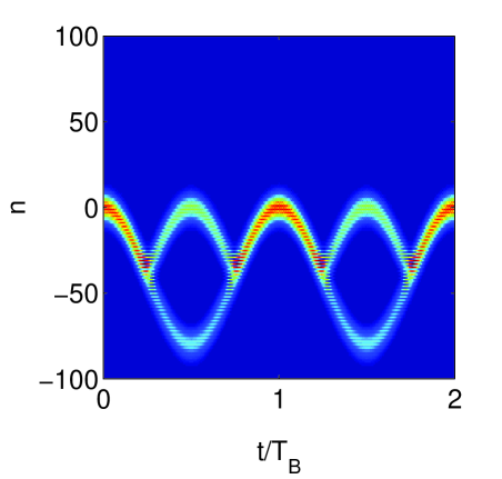
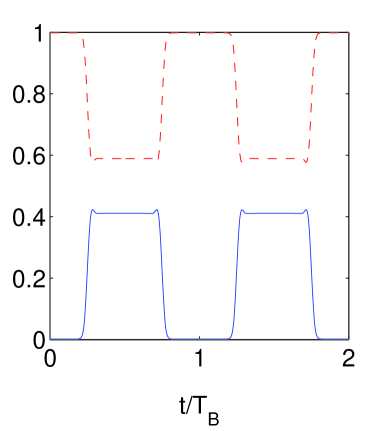
Figure 5: Dynamics of an oscillating Bloch-Zener mode. The left-hand side shows $|\psi|^{2}$ versus ’space’ and time. The right-hand side shows the occupation probability of the lower minband (dashed red line) and the upper band (solid blue line) versus time. The parameters are $\Delta=80$, $dF=1$ and $\delta=6.734$.

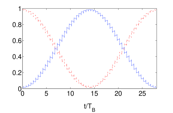
Figure 6: Occupation probability of the lower minband (dashed red line) and the upper band (solid blue line) for an oscillatory mode versus time. The parameters are $\Delta=80$, $dF=1$ and $\delta=17.19$.

When $\frac{dF-2E_{0}}{dF}\pi$ is close to $2\pi$, the cosine in equations (76) and (77) changes very slightly after each period $T_{1}$, which illustrates the cosine-like behaviour of the occupation probability very clearly. This is shown in figure 6 for an oscillatory mode with the same initial condition as above. By the choice of the parameters $\Delta$, $dF$ and $\delta$ we get $E_{0}=-0.5178$ and hence

$$\frac{T_{2}}{T_{1}}=\frac{56}{57}\,.$$ (78)

Thus we get a reconstruction at multiples of $T_{BZ}=28T_{B}$. The slowly varying oscillation of the occupation between the bloch bands is similar to the Rabi oscillations for a two level system.

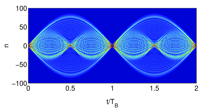
Figure 7: Dynamics of a breathing mode. The modulus of the wave function $|\psi|$ is plotted versus ’space’ and time. The parameters are $\Delta=80$, $dF=1$ and $\delta=6.734$.

Let us now consider a wave packet that is initially located at a single site (see figure 7). In the case of a single-band system ($\delta=0$) one finds a breathing behaviour: The width of the wave packet oscillates strongly, while its position remains constant [12]. The parameters are chosen as in figure 5, so that reconstruction happens again after integer multiples of $T_{BZ}=T_{B}$. One observes that the enveloping structure with the period $T_{BZ}=T_{B}$ is overlayed by a breathing mode of smaller amplitude, which can be interpreted as a fraction of the wave packet staying in one band all the time. Therefore the characteristic period of this part is $T_{1}=T_{B}/2$. The gradient of the dispersion relation of a band changes at the edge of the Brillouin zone if there is no band transition. Therefore the direction of motion given by the group velocity changes after $T_{1}=T_{B}/2$ and the breathing amplitude of this part of the wave packet is thus smaller than the amplitude of the complete breathing mode.

4.5 Beam splitters

The Bloch-Zener transition between the two minibands can be used to construct a matter wave beam splitter with controllable ’transmission’. To see this, note that interband transitions mainly take place at the edge of the Brillouin zone (see figure 2). In the case of a partial band transition, the wave packet is spatially separated, as illustrated in figure 5.

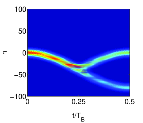
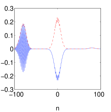
Figure 8: Splitting of a gaussian wave packet in ’real’ space. The left hand side shows $|\psi|^{2}$ versus ’space’ and time. The right hand side shows the absolute value (red dashed line) and the real part (blue solid line) of the wave function at $t=0.5\,T_{B}$ versus ’space’. The parameters are $\Delta=80$, $dF=1$ and $\delta=6.734$.

The time evolution of the squared modulus of a wave packet with a broad initial distribution $\sim\rme^{-n^{2}/100}$ is shown in figure 8. At time $t=0.5\,T_{B}$, both parts of the wave packet have a gaussian profile, but the lower part of the wave function consists of states with opposite momentum. Hence the phase of the wave function and therefore its real part oscillate strongly. Usually both parts merge again after a full Bloch period $T_{B}$ (cf. figure 5). However, a permanent splitting of the wave packet can be obtained by flipping the sign of $F$ at $t=0.5\,T_{B}$. Thereby both parts of the wave packet are transported in opposite directions (compare [23]). This effect is shown in figure 9 (same initial state as above). After flipping the field $F$, the external force is constant and therefore both splitted wave packets continue their Bloch-Zener oscillations separately. Furthermore it is possible to control the occupation of each branch by the choice of $\delta$.

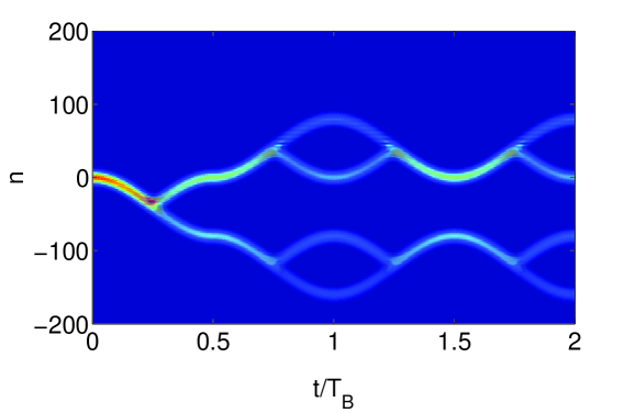
Figure 9: Splitting of a gaussian wave packet in ’real’ space. Shown is $|\psi|^{2}$ versus ’space’ $n$ and time $t$. The parameters are $\Delta=80$, $d=1$, $\delta=6.734$ and $|F|=1$.

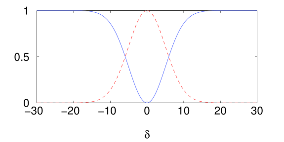
Figure 10: Occupation probability of the above gaussian wave packet at $t=0.5\,T_{B}$ versus $\delta$. The red dashed line shows the occupation in the interval $-100\leq n\leq-40$ whereas the blue solid line shows the occupation in the interval $-41\leq n\leq 20$. The parameters are $\Delta=80$, $d=1$, and $F=1$.

The transition probability at $t=0.5\,T_{B}$ for a wave packet initially located in a single band is in good approximation given by the Landau-Zener formula (58). The numerical results for the occupation of the different branches (compare figure 8) at $t=0.5\,T_{B}$ versus $\delta$ are shown in figure 10. Such a controlled manipulation of the band gap can be achieved, for example, in optical lattices. In this case it is also possible to construct a beam splitter in a different way, namely by ’switching off’ $\delta$ completely at $t=0.5\,T_{B}$. Instead of Bloch-Zener oscillations, simple Bloch oscillations will appear with the advantage that the two wave packets can be separated by low-loss transport as described in [12, 23]. In any case it is possible to control the amplitude of each of the splitted wave packets by the choice of $\delta$.

5 Conclusion and Outlook

In conclusion, we have investigated the interplay between Bloch oscillations and Zener tunneling between the Bloch bands. To this end we considered a special tight-binding model under the influence of a static external field. This model satisfactorily describes the dynamics of a more realistic system as demonstrated in a comparison with exact numerical computations [23]. An additional period-doubled potential leads to a splitting of the ground band into two minibands in the field-free case. For a non-zero external field, the spectrum of the system consists of exactly two Wannier-Stark ladders. The dependence of the energy offset between the two ladders on the system parameters was discussed in detail.

The dynamics of the system is governed by two time-scales, the Bloch period $T_{1}$ defined in equation (70) and the period $T_{2}$ of the Zener oscillation between the two energy ladders introduced in equation (71). If the two periods are commensurable, a wave packet will reconstruct periodically up to a global phase. The occupation of the two minibands at multiples of the Bloch period $T_{1}$ oscillates sinusoidally in time. Furthermore it was shown that the dynamics of the system can be reduced to a Whittaker-Hill differential equation. Unfortunately few analytic results are available for the solutions of this differential equation.

Finally some numerical examples of Bloch-Zener oscillations were given. It was shown that Bloch-Zener oscillations in a double-periodic potential can be used to construct matter wave beam splitters, e.g. for cold atoms in optical lattices.

A further important application of a Bloch-Zener oscillation as shown in figure 5 is the construction of a matter wave interferometer by introducing an additional external potential into one of the two branches of the splitted wave packet. Hence the band transitions act as beam splitters in a Mach-Zehnder interferometer setup. These aspects will be discussed in more detail in a future publication [23].

Appendix

The time independent Schrödinger equation in the basis of Bloch waves consists of two coupled differential equations (6) and (7). Using the ansatz

$$\langle\chi_{0,\kappa}|\Psi\rangle=Q_{\kappa}\,\rme^{-\rmi\kappa E/F}\qquad\mbox{and}\qquad\langle\chi_{1,\kappa}|\Psi\rangle=P_{\kappa}\,\rme^{-\rmi\kappa E/F}$$ (79)

we will show that in the case of a two-band system there exist exactly two energy ladders. A similar proof can be found in [24] for a different system. Substituting (79) into equations (6) and (7) we obtain

$$\frac{\partial}{\partial\kappa}\left(\begin{array}[]{*{2}{c}}Q_{\kappa}\\ P_{\kappa}\\ \end{array}\right)=\frac{\rmi}{F}\left(\begin{array}[]{*{2}{c}}E_{0,\kappa}-dF&M_{\kappa}^{*}\\ M_{\kappa}&E_{1,\kappa}\\ \end{array}\right)\left(\begin{array}[]{*{2}{c}}Q_{\kappa}\\ P_{\kappa}\\ \end{array}\right)=\mathbf{A}_{\kappa}\left(\begin{array}[]{*{2}{c}}Q_{\kappa}\\ P_{\kappa}\\ \end{array}\right)\,.$$ (80)

The dispersion relations $E_{0,\kappa}$, $E_{1,\kappa}$ and the reduced transition matrix element $M_{\kappa}$ are $\pi/d$-periodic. Therefore we can apply Floquet’s theorem, which says that a system of linear homogeneous differential equations with periodic coefficients as given above is solved by a fundamental system of the structure

$$\mathbf{X}_{\kappa}=\mathbf{Y}_{\kappa}\,\rme^{\rmi\kappa\mathbf{Z}}\,,$$ (81)

where $\mathbf{Y}_{\kappa}$ is a $\pi/d$-periodic $2\times 2$ - matrix and $\mathbf{Z}$ is a constant complex $2\times 2$ - matrix. Let the eigenvalues of $\mathbf{Z}$, called characteristic exponents, be denoted by $z_{0}$ and $z_{1}$. They are only defined up to multiples of $2d$. Multiplication of the fundamental system (81) with the eigenvectors of $\mathbf{Z}$ from the right leads to

$$\left(\begin{array}[]{*{2}{c}}Q_{\kappa,n}\\ P_{\kappa,n}\\ \end{array}\right)=\rme^{\rmi\kappa z_{n}}\left(\begin{array}[]{*{2}{c}}f_{\kappa,n}\\ g_{\kappa,n}\\ \end{array}\right)$$ (82)

with $\pi/d$-periodic functions $f_{\kappa,n}$ and $g_{\kappa,n}$. Here, $n=0,1$ distinguishes both possible eigenvectors. Because $\langle\chi_{0,\kappa}|\Psi\rangle$ and $\langle\chi_{1,\kappa}|\Psi\rangle$ have to be $\pi/d$-periodic, too, the phases are given by

$$-\rmi\frac{\pi}{d}\frac{E}{F}+\rmi\frac{\pi}{d}z_{n}=-\rmi 2\pi m$$ (83)

with $m\in\mathbb{Z}$. The energies are therefore

$$E_{n,m}=2mdF+Fz_{n}\,.$$ (84)

Obviously, there exist exactly two different energy ladders as long as the eigenvalues of $\mathbf{Z}$ are distinct. Due to the fact that the Hamiltonian (1) is hermitian, the energies $E_{n,m}$ , and thus the $z_{n}$, are real numbers.

References

References

• [1] F. Bloch, Z. Phys 52 (1928) 555
• [2] J. Feldmann, K. Leo, J. Shah, B. A. B. Miller, J. E. Cunningham, T. Meier, G. von Plessen, A. Schulze, P. Thomas, and S. Schmitt-Rink, Phys. Rev. B 46 (1992) 7252
• [3] M. Ben Dahan, E. Peik, J. Reichel, Y. Castin, and C. Salomon, Phys. Rev. Lett. 76 (1996) 4508
• [4] T. Pertsch, P. Dannberg, W. Elflein, A. Bräuer, and F. Lederer, Phys. Rev. Lett. 83 (1999) 4752
• [5] R. Morandotti, U. Peschel, J. S. Aitchinson, H. S. Eisenberg, and Y. Silberberg, Phys. Rev. Lett. 83 (1999) 4756
• [6] L. Gutiérrez, A. Díaz-de-Anda, J. Flores, R. A. Méndez-Sanchez, G. Monsivais and A. Morales, in preparation (2006)
• [7] C. Zener, Proc. Roy. Soc. Lond. A 145 (1934) 523
• [8] B. P. Anderson and M. A. Kasevich, Science 282 (1998) 1686
• [9] B. Rosam, K. Leo, M. Glück, F. Keck, H. J. Korsch, F. Zimmer, and K. Köhler, Phys. Rev. B 68 (2003) 125301
• [10] H. Trompeter, T. Pertsch, F. Lederer, D. Michaelis, U. Streppel, A. Brauer, and U. Peschel, Phys. Rev. Lett. 96 (2006) 023901
• [11] M. Glück, A. R. Kolovsky, and H. J. Korsch, Phys. Rep. 366 (2002) 103
• [12] T. Hartmann, F. Keck, H. J. Korsch, and S. Mossmann, New J. Phys. 6 (2004) 2
• [13] V. I. Kovanis and V. M. Kenkre, Phys. Lett. A 130 (1988) 147
• [14] X.-G. Zhao, J. Phys.: Condens. Matter 3 (1991) 6021
• [15] X.-G. Zhao, J. Phys.: Condens. Matter 9 (1997) L385
• [16] A. R. Kolovsky and H. J. Korsch, Phys. Rev. A 67 (2003) 063601
• [17] D. Witthaut, F. Keck, H. J. Korsch, and S. Mossmann, New J. Phys. 6 (2004) 41
• [18] M. Abramowitz and I. A. Stegun, Handbook of Mathematical Functions, Dover Publications, Inc., New York, 1972
• [19] H. J. Korsch and S. Mossmann, Phys. Lett. A 317 (2003) 54
• [20] K. M. Urwin and F. M. Arscott, Proc. Roy. Soc. Edinburgh 69 (1970) 28
• [21] L. D. Landau, Phys. Z. Sowjet. 1 (1932) 88
• [22] C. Zener, Proc. Roy. Soc. Lond. A 137 (1932) 696
• [23] B. M. Breid, D. Witthaut, and H. J. Korsch, in preparation (2006)
• [24] H. Fukuyama, R. A. Bari, and H. C. Fogedby, Phys. Rev. B 8 (1973) 5579