Robust observer for uncertain linear quantum systems

Abstract

In the theory of quantum dynamical filtering, one of the biggest issues is that the underlying system dynamics represented by a quantum stochastic differential equation must be known exactly in order that the corresponding filter provides an optimal performance; however, this assumption is generally unrealistic. Therefore, in this paper, we consider a class of linear quantum systems subjected to time-varying norm-bounded parametric uncertainties and then propose a robust observer such that the variance of the estimation error is guaranteed to be within a certain bound. Although in the linear case much of classical control theory can be applied to quantum systems, the quantum robust observer obtained in this paper does not have a classical analogue due to the system’s specific structure with respect to the uncertainties. Moreover, by considering a typical quantum control problem, we show that the proposed robust observer is fairly robust against a parametric uncertainty of the system even when the other estimators—the optimal Kalman filter and risk-sensitive observer—fail in the estimation.

I Introduction

Quantum filtering theory was pioneered by Belavkin in remarkable papers belavkin1 ; belavkin2 ; belavkin3 and was more lucidly reconsidered by Bouten et al. luc1 ; luc2 . This theory is now recognized as a very important basis for the development of various engineering applications of the quantum theory such as quantum feedback control wiseman1 ; doherty1 ; thomsen ; geremia1 ; ramon1 ; wiseman2 , quantum dynamical parameter estimation mabuchi ; geremia2 ; stockton , and quantum information processing ahn1 ; ahn2 .

We here provide a brief summary of the quantum filtering theory by using the same notations as those in luc1 ; luc2 . Let us consider an open system in contact with a field, particularly a vacuum electromagnetic field. This interaction is completely described by a unitary operator $\hat{U}_{t}$ that obeys the following quantum stochastic differential equation (QSDE) termed the Hudson-Parthasarathy equation hudson :

$$\hbar d\hat{U}_{t}=\Big{[}\big{(}-{\rm i}\hat{H}-\frac{1}{2}\hat{c}^{\dagger}\hat{c}\big{)}dt+\hat{c}d\hat{B}_{t}^{\dagger}-\hat{c}^{\dagger}d\hat{B}_{t}\Big{]}\hat{U}_{t},~{}~{}\hat{U}_{0}=\hat{I},$$ (1)

where $\hat{c}$ and $\hat{H}$ are the system operator and Hamiltonian, respectively. The quantum Wiener process $\hat{B}_{t}$, which is a field operator, satisfies the following quantum Ito rule:

$$d\hat{B}_{t}d\hat{B}_{t}=0,~{}d\hat{B}_{t}^{\dagger}d\hat{B}_{t}=0,~{}d\hat{B}_{t}d\hat{B}_{t}^{\dagger}=\hbar dt,~{}d\hat{B}_{t}^{\dagger}d\hat{B}_{t}^{\dagger}=0.$$

The time evolution of any system observable $\hat{X}$ under the interaction (1) is described by the unitary transformation $j_{t}(\hat{X}):=\hat{U}_{t}^{\dagger}\hat{X}\hat{U}_{t}$. The infinitesimal change in this transformation is calculated as

$$\hbar dj_{t}(\hat{X})=j_{t}({\cal L}\hat{X})dt+j_{t}([\hat{c}^{\dagger},\hat{X}])d\hat{B}_{t}+j_{t}([\hat{X},\hat{c}])d\hat{B}_{t}^{\dagger}.$$ (2)

Here, we have defined ${\cal L}\hat{X}:={\rm i}[\hat{H},\hat{X}]+\hat{c}^{\dagger}\hat{X}\hat{c}-\frac{1}{2}\hat{c}^{\dagger}\hat{c}\hat{X}-\frac{1}{2}\hat{X}\hat{c}^{\dagger}\hat{c}$. The field operator after the interaction is determined by $\hat{B}_{t}^{\prime}:=j_{t}(\hat{B}_{t})$. In the homodyne detection scheme, we measure the field operator of the form $Y_{t}:=\hat{B}_{t}^{\prime}+\hat{B}_{t}^{\prime}\mbox{}^{\dagger}$, which results in

$$dY_{t}=j_{t}(\hat{c}+\hat{c}^{\dagger})dt+d\hat{B}_{t}+d\hat{B}_{t}^{\dagger}.$$ (3)

An important fact is that the above observable is self-nondemolition: $[Y_{s},Y_{t}]=0$ for all $s$ and $t$. This implies that the observation is a classical stochastic process. (For this reason, we omit the “hat” on $Y_{t}$, but note that it itself is not a $c$-number.) It is also noteworthy that $Y_{t}$ satisfies the quantum nondemolition (QND) condition, $[Y_{s},j_{t}(\hat{X})]=0~{}\forall s\leq t$, for all system observables $\hat{X}$. Our goal is to obtain the best estimate of the system observable $j_{t}(\hat{X})$ based on the observations $Y_{s}~{}(0\leq s\leq t)$, which generate the Von Neumann algebra ${\cal Y}_{t}={\rm vN}(Y_{s}\hskip 0.85355pt:\hskip 0.85355pt0\leq s\leq t)$. As in the case of the classical filtering theory, the best estimate in the sense of the least mean square error, $\langle{(j_{t}(\hat{X})-X^{\prime})^{2}}\rangle\rightarrow{\rm min.}$, is given by (a version of) the quantum conditional expectation: $X^{\prime}=\pi_{t}(\hat{X}):={\mathbb{P}}(\hskip 1.42271ptj_{t}(\hat{X})\hskip 1.42271pt|\hskip 1.42271pt{\cal Y}_{t}\hskip 1.42271pt)$. Here, the expectation $\langle{\hat{X}}\rangle$ is defined by $\langle{\hat{X}}\rangle:={\rm Tr}\hskip 1.9919pt[\hat{X}(\hat{\rho}\otimes\hat{\Phi})]$, where $\hat{\rho}$ and $\hat{\Phi}$ represent the system quantum state and the field vacuum state, respectively. It should be noted that the following two conditions must hold in order for the above quantum conditional expectation to be defined: First, ${\cal Y}_{t}$ is a commutative algebra, and second, $j_{t}(\hat{X})$ is included in the commutant of ${\cal Y}_{t}$. But these conditions are actually satisfied as shown above. Consequently, the optimal filter for the system dynamics (2) is given by the change in $\pi_{t}(\hat{X})$ as follows:

$$\hbar d\pi_{t}(\hat{X})=\pi_{t}({\cal L}\hat{X})dt+\big{[}\pi_{t}(\hat{X}\hat{c}+\hat{c}^{\dagger}\hat{X})$$

$$\hskip 30.00005pt\mbox{}-\pi_{t}(\hat{X})\pi_{t}(\hat{c}+\hat{c}^{\dagger})\big{]}\big{[}dY_{t}-\pi_{t}(\hat{c}+\hat{c}^{\dagger})dt\big{]}.$$ (4)

We can further incorporate some control terms into the above equation. Typically, a bounded real scalar control input $u_{t}$, which should be a function of the observations $Y_{s}$ up to time $t$, is included in the coefficients of the Hamiltonian. We lastly remark that the conditional system state $\hat{\rho}_{t}$ is associated with the system observable by the relation $\pi_{t}(\hat{X})={\rm Tr}\hskip 1.9919pt(\hat{X}\hat{\rho}_{t})$, which leads to the dynamics of $\hat{\rho}_{t}$ termed the stochastic master equation.

A key assumption in the filtering theory is that perfect knowledge about the system dynamics model (2) is required in order that the filter (I) provides the best estimate of the (controlled) system observable. However, this assumption is generally unrealistic, and we depend on only an approximate model of the system. This not only violates the optimality of the estimation but also possibly leads to the instability of the estimation error dynamics. This problem is well recognized in the classical filtering theory and various alternative estimators for uncertain systems, which are not necessarily optimal but robust to the uncertainty, have been proposed. (We use the term “filter” to refer to only the optimal estimator.) For example, in a risk-sensitive control problem in which an exponential-of-integral cost function is minimized with respect to the control input, it is known that the corresponding risk-sensitive observer enjoys enhanced robustness property to a certain type of system uncertainty jacobson ; bensou ; dupuis . Moreover, by focusing on specific uncertain systems, it is possible to design a robust observer such that the variance of the estimation error is guaranteed to be within a certain bound for all admissible uncertainties petersen1 ; xie ; shaked ; petersen2 .

It is considered that the above mentioned robust estimation methods are very useful in the quantum case since it is difficult to specify the exact parameters of a quantum system in any realistic situation: for instance, the total spin number of a spin ensemble stockton . With this background, James has developed a quantum version of the risk-sensitive observer for both continuous james2 and discrete cases james1 and applied it to design an optimal risk-sensitive controller for a single-spin system. We should remark that, however, the above papers did not provide an example of a physical system such that the quantum risk-sensitive observer is actually more robust than the nominal optimal filter.

Therefore, in this paper, we focus on the robust observer and develop its quantum version. More specifically, we consider a class of quantum linear systems subjected to time-varying norm-bounded parametric uncertainties and obtain a quantum robust observer that guarantees a fixed upper bound on the variance of the estimation error. Although in the linear case much of classical control theory applies to quantum systems, the robust observer obtained in this paper does not have a classical analogue in the following sense. First, unlike the classical case, the error covariance matrix must be symmetrized because of the noncommutativity of the measured system observables. Second, due to the unitarity of quantum evolution, the uncertainties are included in the system representation in a different and more complicated way than those in the classical system considered previously; as a result, both the structure of the quantum robust observer and the proof to derive it differ substantially from those found in petersen1 ; xie ; shaked ; petersen2 . The other contribution of this paper is that it actually provides a quantum system such that both the robust observer and the risk-sensitive observer show better performance in the estimation error than the nominal optimal filter.

This paper is organized as follows. Section II provides a basic description of general linear quantum systems, in which case the optimal filter (I) is termed the quantum Kalman filter. In addition, we derive a linear risk-sensitive observer. In both cases, an explicit form of the optimal control input is provided. The quantum version of the robust observer is provided in Section III. Section IV discusses robustness properties of the proposed robust observer and the risk-sensitive observer by considering a typical quantum control problem—feedback cooling of particle motion. Section V concludes the paper.

We use the following notations: for a matrix $A=(a_{ij})$, the symbols $A^{{\mathsf{T}}}$ and $A^{*}$ represent its transpose and elementwise complex conjugate of $A$, i.e., $A^{\mathsf{T}}=(a_{ji})$ and $A^{*}=(a_{ij}^{*})=(A^{\dagger})^{{\mathsf{T}}}$, respectively; these rules can be applied to any rectangular matrix including column and row vectors. A Hermitian matrix $A=A^{\dagger}$ is positive semidefinite if $v^{\dagger}Av\geq 0$ for any vector $v$; the inequality $A\geq B$ represents the positive semidefiniteness of $A-B$.

II Linear quantum system

II.1 Quantum Kalman filter

In this paper, we consider a single one-dimensional particle interacting with a vacuum electromagnetic field. The extension to the multi-particle case is straightforward wiseman2 . In particular, we focus on the particle position $\hat{q}$ and momentum $\hat{p}$. The system Hamiltonian and operator are respectively given by

$$\hat{H}=\frac{1}{2}\hat{x}^{{\mathsf{T}}}G\hat{x}-\hat{x}^{{\mathsf{T}}}\Sigma Bu_{t},~{}~{}\hat{c}=\tilde{C}\hat{x},$$ (5)

where $\hat{x}=[\hat{q}~{}\hat{p}]^{{\mathsf{T}}}$. Here, $u_{t}\in{\mathbb{R}}$ is the control input, $B\in{\mathbb{R}}^{2}$ is a column vector, and $\tilde{C}\in{\mathbb{C}}^{2}$ is a row vector. The $2\times 2$ matrix $G$ is real symmetric and $\Sigma$ is given by

$$\Sigma=\left[\begin{array}[]{cc}0&1\\ -1&0\\ \end{array}\right].$$

Then, by defining $\hat{x}_{t}=[\hat{q}_{t}~{}\hat{p}_{t}]^{{\mathsf{T}}}=[j_{t}(\hat{q})~{}j_{t}(\hat{p})]^{{\mathsf{T}}}$ and noting the commutation relation $[\hat{q},~{}\hat{p}]={\rm i}\hbar$, the system dynamics (2) leads to the following linear QSDE:

$$d\hat{x}_{t}=A\hat{x}_{t}dt+Bu_{t}dt+{\rm i}\Sigma[\tilde{C}^{{\mathsf{T}}}d\hat{B}_{t}^{\dagger}-\tilde{C}^{\dagger}d\hat{B}_{t}],$$ (6)

where the matrix $A$ is defined by $A:=\Sigma[G+{\rm Im}(\tilde{C}^{\dagger}\tilde{C})]$. The output equation (3) becomes

$$dY_{t}=F\hat{x}_{t}dt+d\hat{B}_{t}+d\hat{B}_{t}^{\dagger},~{}~{}F:=\tilde{C}+\tilde{C}^{*}.$$

It follows from Eq. (I) that the best estimate of the system observable, $\pi_{t}(\hat{x}):=[\pi_{t}(\hat{q})~{}\pi_{t}(\hat{p})]^{{\mathsf{T}}}\in{\mathbb{R}}^{2}$, obeys the following filter equation:

$$d\pi_{t}(\hat{x})=A\pi_{t}(\hat{x})dt+Bu_{t}dt$$

$$\hskip 15.00002pt\mbox{}+\Big{[}\frac{1}{\hbar}V_{t}F^{{\mathsf{T}}}+\Sigma^{{\mathsf{T}}}{\rm Im}(\tilde{C})^{{\mathsf{T}}}\Big{]}(dY_{t}-F\pi_{t}(\hat{x})dt).$$ (7)

In the above equation, $V_{t}$ represents the symmetrized covariance matrix defined by

$$V_{t}:={\mathbb{P}}(\hskip 1.42271pt\hat{P}_{t}\hskip 1.42271pt|\hskip 1.42271pt{\cal Y}_{t}\hskip 1.42271pt)$$

$$\hat{P}_{t}:=\left[\begin{array}[]{cc}\Delta\hat{q}_{t}^{2}&\frac{1}{2}(\Delta\hat{q}_{t}\Delta\hat{p}_{t}+\Delta\hat{p}_{t}\Delta\hat{q}_{t})\\ \frac{1}{2}(\Delta\hat{q}_{t}\Delta\hat{p}_{t}+\Delta\hat{p}_{t}\Delta\hat{q}_{t})&\Delta\hat{p}_{t}^{2}\end{array}\right],$$ (10)

where $\Delta\hat{q}_{t}:=\hat{q}_{t}-\pi_{t}(\hat{q})$ and $\Delta\hat{p}_{t}:=\hat{p}_{t}-\pi_{t}(\hat{p})$. The covariance matrix $V_{t}$ changes in time deterministically according to the following Riccati differential equation:

$$\dot{V}_{t}=AV_{t}+V_{t}A^{{\mathsf{T}}}+D$$

$$\hskip 5.0pt\mbox{}-\frac{1}{\hbar}(V_{t}F^{{\mathsf{T}}}+\hbar\Sigma^{{\mathsf{T}}}{\rm Im}(\tilde{C})^{{\mathsf{T}}})(FV_{t}+\hbar{\rm Im}(\tilde{C})\Sigma),$$

$$V_{0}={\mathbb{P}}(\hskip 1.42271pt\hat{P}_{0}\hskip 1.42271pt|\hskip 1.42271pt{\cal Y}_{0}\hskip 1.42271pt),$$ (12)

where $D:=\hbar\Sigma{\rm Re}(\tilde{C}^{\dagger}\tilde{C})\Sigma^{{\mathsf{T}}}$. Consequently, the optimal filter for the linear quantum system (6) is described by the closed set of equations (II.1) and (II.1), which is termed the quantum Kalman filter doherty1 ; wiseman2 ; geremia2 . A remarkable fact is that the behavior of $V_{t}$ is determined without respect to the output $Y_{t}$. This indicates that we can evaluate the quantum conditional expectation $V_{t}={\mathbb{P}}(\hskip 1.42271pt\hat{P}_{t}\hskip 1.42271pt|\hskip 1.42271pt{\cal Y}_{t}\hskip 1.42271pt)$ by simply calculating the expectation $V_{t}=\langle{\hat{P}_{t}}\rangle$. Actually, as $V_{t}$ evolves deterministically, we can see

$$\langle{\hat{P}_{t}}\rangle=\langle{{\mathbb{P}}(\hskip 1.42271pt\hat{P}_{t}\hskip 1.42271pt|\hskip 1.42271pt{\cal Y}_{t}\hskip 1.42271pt)}\rangle=\langle{V_{t}}\rangle=V_{t}.$$

Now, the quantum version of Linear Quadratic Gaussian (LQG) control problem is addressed as follows. For the linear quantum system driven by the quantum Gaussian noise, we aim to find an optimal control input $u_{t}^{{\rm opt}}$, which is a function of the observations $Y_{s}~{}(0\leq s\leq t)$, such that the following quadratic cost function is minimized:

$$J[u_{t}]=\Big{\langle}\int_{0}^{T}\Big{(}\frac{1}{2}\hat{x}_{t}^{{\mathsf{T}}}M\hat{x}^{\mbox{}}_{t}+\frac{r}{2}u_{t}^{2}\Big{)}dt+\frac{1}{2}\hat{x}_{T}^{{\mathsf{T}}}N\hat{x}_{T}^{\mbox{}}\Big{\rangle}.$$ (13)

The positive semidefinite matrices $M\geq 0,~{}N\geq 0$ and the scalar number $r>0$ reflect our control strategy; For example, if we are strongly restricted in the magnitude of the control input, a large value of $r$ should be chosen. This problem can be solved by using the dynamic programming method. The optimal input is then given by $u_{t}^{{\rm opt}}=-(2/r)B^{{\mathsf{T}}}K_{t}\pi_{t}(\hat{x})$, where the real symmetric matrix $K_{t}$ is a solution to the following Riccati differential equation:

$$\dot{K}_{t}+K_{t}A+A^{{\mathsf{T}}}K_{t}-\frac{2}{r}K_{t}BB^{{\mathsf{T}}}K_{t}+\frac{1}{2}M=O,$$

$$K_{T}=N.$$ (14)

Thus, we observe that the optimal control input $u_{t}^{{\rm opt}}$ is not a function of the entire observation history up to time $t$, but only depends on the solution to the Kalman filter (II.1) and (II.1) at time $t$. A controller that satisfies this desirable property is termed a separated controller. A general discussion on the optimality of the separated control is found in luc3 .

II.2 Quantum risk-sensitive observer

The risk-sensitive control problem was originally formulated by Jacobson within the framework of the classical control theory jacobson , and recently its quantum version was developed by James james1 ; james2 . The purpose is to design an optimal control input such that the following cost function is minimized:

$$J^{\mu}[u_{t}]=\langle\hat{R}_{T}^{\dagger}j_{T}^{\mbox{}}({\rm e}^{\mu\hat{\beta}})\hat{R}_{T}^{\mbox{}}\rangle,$$ (15)

where $\hat{R}_{t}$ is the solution to the operator differential equation $d\hat{R}_{t}/dt=(\mu/2)j_{t}(\hat{\alpha}(u_{t}))\hat{R}_{t}$ and the parameter $\mu\geq 0$ represents the risk-sensitivity. The nonnegative self-adjoint system operators $\hat{\alpha}(u_{t})$ and $\hat{\beta}$ are termed the running and terminal cost operators, respectively. In the classical case where the cost operators are scalar values, i.e., $\hat{\alpha}(u_{t})=\alpha(u_{t})$ and $\hat{\beta}=\beta$, the cost function (15) is reduced to

$$J^{\mu}[u_{t}]=\Big{\langle}{\rm exp}\Big{(}\mu\int_{0}^{T}\alpha(u_{t})dt+\mu\beta\Big{)}\Big{\rangle}.$$

For this reason, Eq. (15) is considered as a natural noncommutative generalization of the exponential-of-integral cost function. James has proved that the quantity (15) is expressed as

$$J^{\mu}[u_{t}]={\mathbb{E}}^{\mu}\Big{[}{\rm exp}\Big{(}\mu\int_{0}^{T}\pi^{\mu}_{t}(\hat{\alpha})dt\Big{)}\pi^{\mu}_{T}({\rm e}^{\mu\hat{\beta}})\Big{]},$$ (16)

where ${\mathbb{E}}^{\mu}$ denotes the expectation with respect to a certain classical probability distribution (see james2 ) and $\pi^{\mu}_{t}(\bullet)$ is a risk-dependent estimate of the system observable. The estimator is determined by the following equation:

$$\hbar d\pi^{\mu}_{t}(\hat{X})=\pi^{\mu}_{t}({\cal L}\hat{X})dt$$

$$\hskip 40.00006pt\mbox{}+\frac{\mu}{2}\big{[}\pi^{\mu}_{t}(\hat{X}\hat{\alpha}+\hat{\alpha}\hat{X})-2\pi^{\mu}_{t}(\hat{X})\pi^{\mu}_{t}(\hat{\alpha})\big{]}dt$$

$$\hskip 40.00006pt\mbox{}+\big{[}\pi^{\mu}_{t}(\hat{X}\hat{c}+\hat{c}^{\dagger}\hat{X})-\pi^{\mu}_{t}(\hat{X})\pi^{\mu}_{t}(\hat{c}+\hat{c}^{\dagger})\big{]}$$

$$\hskip 60.00009pt\times\big{[}dY_{t}-\pi^{\mu}_{t}(\hat{c}+\hat{c}^{\dagger})dt\big{]}.$$ (17)

This differs from the filtering equation (I) in that the risk-dependent term is added to it. Therefore, $\pi^{\mu}_{t}(\hat{X})$ is no longer the optimal estimate of the system observable. However, the risk-dependent term is indeed necessary in order for the cost function (15) to be expressed only in terms of quantities defined on the system space that is driven by the output $Y_{t}$. This implies that our knowledge about the system is tempered by purpose.

We now apply the above mentioned risk-sensitive control theory to the linear system (6) with the following cost operators:

$$\hat{\alpha}(u_{t})=\frac{1}{2}\hat{x}^{{\mathsf{T}}}M\hat{x}+\frac{r}{2}u_{t}^{2},~{}~{}\hat{\beta}=\frac{1}{2}\hat{x}^{{\mathsf{T}}}N\hat{x},$$

where $M$ and $N$ are $2\times 2$ positive semidefinite matrices and $r>0$. Then, through a lengthy calculation we obtain the corresponding observer equation as follows:

$$d\pi^{\mu}_{t}(\hat{x})=(A+\mu V^{\mu}_{t}M)\pi^{\mu}_{t}(\hat{x})dt+Bu_{t}dt$$

$$\mbox{}+\Big{[}\frac{1}{\hbar}V^{\mu}_{t}F^{{\mathsf{T}}}+\Sigma^{{\mathsf{T}}}{\rm Im}(\tilde{C})^{{\mathsf{T}}}\Big{]}(dY_{t}-F\pi^{\mu}_{t}(\hat{x})dt),$$ (18)

where the time evolution of the symmetrized covariance matrix $V^{\mu}_{t}$ is given by

$$\dot{V}^{\mu}_{t}=AV^{\mu}_{t}+V^{\mu}_{t}A^{{\mathsf{T}}}+D$$

$$\hskip 5.0pt\mbox{}-\frac{1}{\hbar}(V^{\mu}_{t}F^{{\mathsf{T}}}+\hbar\Sigma^{{\mathsf{T}}}{\rm Im}(\tilde{C})^{{\mathsf{T}}})(FV^{\mu}_{t}+\hbar{\rm Im}(\tilde{C})\Sigma),$$

$$\hskip 5.0pt\mbox{}+\mu(V^{\mu}_{t}MV^{\mu}_{t}-\frac{\hbar^{2}}{4}\Sigma^{{\mathsf{T}}}M\Sigma),$$

$$V^{\mu}_{0}={\mathbb{P}}(\hskip 1.42271pt\hat{P}_{0}\hskip 1.42271pt|\hskip 1.42271pt{\cal Y}_{0}\hskip 1.42271pt).$$ (19)

Consequently, the risk-sensitive observer (II.2) in linear case reduces to the closed set of equations, (II.2) and (II.2). We also see that the cost function (16) is calculated as

$$J^{\mu}[u_{t}]={\mathbb{E}}^{\mu}\Big{[}{\rm exp}\Big{(}\mu\int_{0}^{T}(\frac{1}{2}\pi^{\mu}_{t}(\hat{x})^{{\mathsf{T}}}M\pi^{\mu}_{t}(\hat{x})+\frac{r}{2}u_{t}^{2})dt\Big{)}$$

$$\hskip 30.00005pt\mbox{}\times{\rm exp}\Big{(}\mu\int_{0}^{T}\frac{1}{2}{\rm Tr}\hskip 1.9919pt(MV_{t}^{\mu})dt\Big{)}\pi^{\mu}_{T}({\rm e}^{\mu\hat{\beta}})\Big{]}.$$

Note that the second integral in the above equation is a constant term as $V^{\mu}_{t}$ is deterministic. This is completely a classical controller design problem and was already solved by Jacobson jacobson ; the optimal control input that minimizes $J^{\mu}[u_{t}]$ is given by

$$u_{t}^{{\rm opt}}=-\frac{2}{r}B^{{\mathsf{T}}}K^{\mu}_{t}\pi^{\mu}_{t}(\hat{x}),$$

where $K^{\mu}_{t}$ satisfies the following Riccati differential equation

$$\dot{K}^{\mu}_{t}+K^{\mu}_{t}A+A^{{\mathsf{T}}}K^{\mu}_{t}-\frac{2}{r}K^{\mu}_{t}BB^{{\mathsf{T}}}K^{\mu}_{t}+\frac{1}{2}M$$

$$\mbox{}+2\mu K^{\mu}_{t}\Big{[}\frac{1}{\hbar}V^{\mu}_{t}F^{{\mathsf{T}}}+\Sigma^{{\mathsf{T}}}{\rm Im}(\tilde{C})^{{\mathsf{T}}}\Big{]}\Big{[}\frac{1}{\hbar}FV^{\mu}_{t}+{\rm Im}(\tilde{C})\Sigma\Big{]}K^{\mu}_{t}$$

$$\mbox{}+\mu(K^{\mu}_{t}V^{\mu}_{t}M+MV^{\mu}_{t}K^{\mu}_{t})=O,$$

$$K_{T}^{\mu}=\frac{1}{2}\big{[}(I-\mu NV^{\mu}_{T})^{-1}N+N(I-\mu V^{\mu}_{T}N)^{-1}\big{]}.$$ (20)

Therefore, $u_{t}^{{\rm opt}}$ is a separated controller composed of the solutions to the observer equation (II.2) and the two coupled Riccati equations (II.2) and (II.2). It is notable that these set of equations are identical to those in the quantum LQG optimal control problem when the risk parameter $\mu$ is zero. In this sense, the LQG optimal controller is sometimes referred to as the linear risk-neutral controller.

III Robust observer for uncertain linear quantum systems

This paper deals with a linear quantum system such that specific uncertainties are included in the system Hamiltonian $\hat{H}$ and the system operator $\hat{c}$ as follows:

$$\hat{H}=\frac{1}{2}\hat{x}^{{\mathsf{T}}}(G+\Delta G_{t})\hat{x}-\hat{x}^{{\mathsf{T}}}\Sigma Bu_{t},$$

$$\hat{c}=(\tilde{C}+\Delta\tilde{C}_{t})\hat{x},$$

where the real symmetric matrix $\Delta G_{t}$ and the complex row vector $\Delta\tilde{C}_{t}$ represent time-varying parametric uncertainties that satisfy the following bounds:

$$(\Delta G_{t})^{2}\leq gI,$$ (21)

$$({\rm Re}\Delta\tilde{C}_{t})^{{\mathsf{T}}}({\rm Re}\Delta\tilde{C}_{t})\leq r_{1}I,~{}~{}({\rm Im}\Delta\tilde{C}_{t})^{{\mathsf{T}}}({\rm Im}\Delta\tilde{C}_{t})\leq r_{2}I.$$

Here, the nonnegative scalar constants $r_{1},r_{2}$, and $g$ are known ($I$ denotes the $2\times 2$ identity matrix). By defining

$$\Delta A_{t}:=\Sigma\Delta G_{t}+\Sigma{\rm Im}\Big{[}\tilde{C}^{\dagger}\Delta\tilde{C}_{t}+\Delta\tilde{C}_{t}^{\dagger}\tilde{C}+\Delta\tilde{C}_{t}^{\dagger}\Delta\tilde{C}_{t}\Big{]},$$

the dynamics of the system observable $\hat{x}_{t}=[\hat{q}_{t}~{}\hat{p}_{t}]^{{\mathsf{T}}}=[j_{t}(\hat{q})~{}j_{t}(\hat{p})]^{{\mathsf{T}}}$ is represented as

$$d\hat{x}_{t}=(A+\Delta A_{t})\hat{x}_{t}dt+Bu_{t}dt$$

$$\mbox{}+{\rm i}\Sigma\big{[}(\tilde{C}+\Delta\tilde{C}_{t})^{{\mathsf{T}}}d\hat{B}_{t}^{\dagger}-(\tilde{C}+\Delta\tilde{C}_{t})^{\dagger}d\hat{B}_{t}\big{]}.$$ (23)

Moreover, the uncertainty is also included in the output equation (3) as follows:

$$dY_{t}=(F+\Delta F_{t})\hat{x}_{t}dt+d\hat{B}_{t}+d\hat{B}_{t}^{\dagger},$$

$$\Delta F_{t}:=\Delta\tilde{C}_{t}+\Delta\tilde{C}_{t}^{*}.$$ (24)

Here, we should remark that the drift and diffusion terms in Eq. (III) and the output equation (III) are affected by the common uncertainty $\Delta\tilde{C}_{t}$. This is because the quantum evolution is restricted to satisfy unitarity and the system matrices are thus strongly connected with each other. This is indeed an intrinsic feature of quantum systems that is not seen in general classical systems.

Motivated from the structure of the Kalman filter (II.1), we aim to design a linear observer of the form

$$dx_{t}=Rx_{t}dt+Bu_{t}dt+kdY_{t},$$ (25)

where $R$ and $k$ are a matrix and a vector to be determined such that the variance of the estimation error is guaranteed to be within a certain bound. The vector $x_{t}=[q_{t}\hskip 5.69046ptp_{t}]^{{\mathsf{T}}}\in{\mathbb{R}}^{2}$ represents the estimate of the system observable $\hat{x}_{t}$. Note that, as in the case of the risk-sensitive observer, $x_{t}$ is not necessarily the optimal estimate of $\hat{x}_{t}$. Furthermore, we here assume that the control input $u_{t}$ is fixed to a linear function of the observer state, $u_{t}=Lx_{t}$, where $L$ is a row vector with the size $2$. Then, an explicit form of $(R,k)$ that enjoys a guaranteed estimation error bound is provided in the following theorem. We remark again that the theorem can be easily generalized to the multi-particle case.

Theorem 1.  Suppose there exist positive scalars $\delta_{i}~{}(i=1,2)$ and $\epsilon_{i}~{}(i=1,\ldots,8)$ such that the following two coupled Riccati equations have positive definite solutions $P_{1}>0$ and $P_{2}>0$:

$$(A+BL)P_{1}+P_{1}(A+BL)^{{\mathsf{T}}}+P_{1}Q_{1}P_{1}$$

$$\mbox{}+D^{\prime}+\delta_{1}I=O,$$ (26)

$$A^{\prime}P_{2}+P_{2}A^{\prime}\mbox{}^{{\mathsf{T}}}+D^{\prime}+\delta_{2}I$$

$$\mbox{}-\frac{1}{\mu_{2}}(P_{2}F^{\prime}\mbox{}^{{\mathsf{T}}}+\mu_{1}\Sigma^{{\mathsf{T}}}{\rm Im}(\tilde{C})^{{\mathsf{T}}})(F^{\prime}P_{2}+\mu_{1}{\rm Im}(\tilde{C})\Sigma)$$

$$\mbox{}-P_{2}(L^{{\mathsf{T}}}B^{{\mathsf{T}}}P_{1}^{-1}+P_{1}^{-1}BL)P_{2}=O,$$ (27)

where the matrices $A^{\prime}$ and $D^{\prime}$ and the vector $F^{\prime}$ are defined by

$$A^{\prime}:=A+(D+Q_{2}+Q_{3})P_{1}^{-1},~{}~{}D^{\prime}:=D+Q_{2}+Q_{3},$$

$$F^{\prime}:=F+\mu_{1}{\rm Im}(\tilde{C})\Sigma P_{1}^{-1}.$$

The definition of the matrices $Q_{i}~{}(i=1,2,3)$ are given in Appendix A: Eqs. (73), (A), and (84). The scalars $\mu_{1}$ and $\mu_{2}$ are given by $\mu_{1}=\hbar+4r_{1}/\epsilon_{2}$ and $\mu_{2}=\hbar+8r_{1}/\epsilon_{2}+\hbar\epsilon_{8}$, respectively. Then, the observer

$$dx_{t}=(A^{\prime}-P_{2}L^{{\mathsf{T}}}B^{{\mathsf{T}}}P_{1}^{-1})x_{t}dt+Bu_{t}dt$$

$$\mbox{}+\frac{1}{\mu_{2}}\Big{[}P_{2}F^{\prime}\mbox{}^{{\mathsf{T}}}+\mu_{1}\Sigma^{{\mathsf{T}}}{\rm Im}(\tilde{C})^{{\mathsf{T}}}\Big{]}(dY_{t}-F^{\prime}x_{t}dt)$$ (28)

generates the estimate $x_{t}=[q_{t}\hskip 5.69046ptp_{t}]^{{\mathsf{T}}}$ that satisfies

$$\lim_{t\rightarrow\infty}\Big{\langle}(\hat{q}_{t}-q_{t})^{2}+(\hat{p}_{t}-p_{t})^{2}\Big{\rangle}\leq{\rm Tr}\hskip 1.9919ptP_{2},$$ (29)

for all admissible uncertainties.

Proof.  We consider the augmented variable $\bar{z}_{t}=[\hat{x}_{t}~{}\hat{x}_{t}-x_{t}]^{{\mathsf{T}}}$, where $\hat{x}_{t}$ and $x_{t}$ satisfy Eqs. (III) and (25), respectively. Then, $\bar{z}_{t}$ obeys the following linear QSDE:

$$d\bar{z}_{t}=(\bar{A}+\Delta\bar{A}_{t})\bar{z}_{t}dt+\bar{b}_{\Delta}d\hat{B}_{t}^{\dagger}+\bar{b}_{\Delta}^{*}d\hat{B}_{t},$$ (30)

where

$$\bar{A}=\left[\begin{array}[]{cc}A+BL&-BL\\ A-R-kF&R\\ \end{array}\right],\Delta\bar{A}_{t}=\left[\begin{array}[]{cc}\Delta A_{t}&O\\ \Delta A_{t}-k\Delta F_{t}&O\\ \end{array}\right],$$ (35)

$$\bar{b}_{\Delta}=\left[\begin{array}[]{c}{\rm i}\Sigma(\tilde{C}+\Delta\tilde{C}_{t})^{{\mathsf{T}}}\\ {\rm i}\Sigma(\tilde{C}+\Delta\tilde{C}_{t})^{{\mathsf{T}}}-k\\ \end{array}\right].$$ (38)

Let us now consider the symmetrized covariance matrix of $\bar{z}$; $\bar{V}_{nm}=\langle{\bar{z}_{n}\bar{z}_{m}+\bar{z}_{m}\bar{z}_{n}}\rangle/2,~{}(n,m=1,\ldots,4)$. This satisfies the following generalized uncertainty relation:

$$\langle{\bar{z}_{t}\bar{z}_{t}^{{\mathsf{T}}}}\rangle=\bar{V}_{t}+\frac{{\rm i}\hbar}{2}\bar{\Sigma}\geq 0,~{}~{}\bar{\Sigma}:=\left[\begin{array}[]{cc}\Sigma&\Sigma\\ \Sigma&\Sigma\\ \end{array}\right].$$

Noting $\hat{B}_{t}\hat{\Phi}=0$ and the quantum Ito rule $d\hat{B}_{t}d\hat{B}_{t}^{\dagger}=\hbar dt$, the time evolution of $\bar{V}_{t}$ is calculated as

$$\frac{d}{dt}\bar{V}_{t}=(\bar{A}+\Delta\bar{A}_{t})\langle{\bar{z}_{t}\bar{z}_{t}^{{\mathsf{T}}}}\rangle+\langle{\bar{z}_{t}\bar{z}_{t}^{{\mathsf{T}}}}\rangle(\bar{A}+\Delta\bar{A}_{t})^{{\mathsf{T}}}+\hbar\bar{b}_{\Delta}^{*}\bar{b}_{\Delta}^{{\mathsf{T}}}$$

$$\hskip 8.00003pt=(\bar{A}+\Delta\bar{A}_{t})\Big{[}\bar{V}_{t}+\frac{{\rm i}\hbar}{2}\bar{\Sigma}\Big{]}$$

$$\hskip 20.00003pt\mbox{}+\Big{[}\bar{V}_{t}+\frac{{\rm i}\hbar}{2}\bar{\Sigma}\Big{]}(\bar{A}+\Delta\bar{A}_{t})^{{\mathsf{T}}}+\hbar\bar{b}_{\Delta}^{*}\bar{b}_{\Delta}^{{\mathsf{T}}}$$

$$\hskip 8.00003pt=(\bar{A}+\Delta\bar{A}_{t})\bar{V}_{t}+\bar{V}_{t}(\bar{A}+\Delta\bar{A}_{t})^{{\mathsf{T}}}+\bar{D}+\Delta\bar{D}_{t}.$$

The matrices $\bar{D}$ and $\Delta\bar{D}_{t}$ are given by

$$\bar{D}=\left[\begin{array}[]{cc}D&D\\ D&D\\ \end{array}\right]-\hbar\left[\begin{array}[]{cc}O&mk^{{\mathsf{T}}}\\ km^{{\mathsf{T}}}&km^{{\mathsf{T}}}+mk^{{\mathsf{T}}}-kk^{{\mathsf{T}}}\\ \end{array}\right],$$ (43)

$$\Delta\bar{D}_{t}=\left[\begin{array}[]{cc}\Delta D_{t}&\Delta D_{t}\\ \Delta D_{t}&\Delta D_{t}\\ \end{array}\right]-\hbar\left[\begin{array}[]{cc}O&\Delta m_{t}k^{{\mathsf{T}}}\\ k\Delta m_{t}^{{\mathsf{T}}}&k\Delta m_{t}^{{\mathsf{T}}}+\Delta m_{t}k^{{\mathsf{T}}}\\ \end{array}\right],$$ (48)

where

$$\Delta D_{t}:=\hbar\Sigma{\rm Re}\Big{[}\tilde{C}^{\dagger}\Delta\tilde{C}_{t}+\Delta\tilde{C}_{t}^{\dagger}\tilde{C}+\Delta\tilde{C}_{t}^{\dagger}\Delta\tilde{C}_{t}\Big{]}\Sigma^{{\mathsf{T}}},$$

$$m:=\Sigma^{{\mathsf{T}}}{\rm Im}(\tilde{C})^{{\mathsf{T}}},~{}~{}\Delta m_{t}:=\Sigma^{{\mathsf{T}}}{\rm Im}(\Delta\tilde{C}_{t})^{{\mathsf{T}}}.$$

Our goal is to design $R$ and $k$ such that the condition

$$\exists\bar{X}>0,$$

$$\mbox{s.t.}~{}~{}(\bar{A}+\Delta\bar{A}_{t})\bar{X}+\bar{X}(\bar{A}+\Delta\bar{A}_{t})^{{\mathsf{T}}}+\bar{D}+\Delta\bar{D}_{t}<0$$ (49)

is satisfied for all admissible uncertainties; in this case, it follows from the lemma shown in Appendix B that the relation $\lim_{t\rightarrow\infty}\bar{V}_{t}\leq\bar{X}$ is satisfied. For this purpose, we utilize the following matrix inequalities: For all $\bar{X}$ and the uncertain matrices satisfying Eqs. (21) and (III), we have

$$\Delta\bar{A}_{t}\bar{X}+\bar{X}\Delta\bar{A}_{t}^{{\mathsf{T}}}\leq\bar{X}\bar{Q}_{1}\bar{X}+\bar{Q}_{2},$$ (50)

$$\Delta\bar{D}_{t}\leq\bar{Q}_{3}.$$ (51)

The proof of the above inequalities and the definition of the matrices $\bar{Q}_{i}~{}(i=1,2,3)$ are given in Appendix A. Therefore, the condition (III) holds for all admissible uncertainties if there exists a positive definite matrix $\bar{X}>0$ such that the following Riccati inequality holds:

$$\bar{\Psi}:=\bar{A}\bar{X}+\bar{X}\bar{A}^{{\mathsf{T}}}+\bar{X}\bar{Q}_{1}\bar{X}+\bar{D}+\bar{Q}_{2}+\bar{Q}_{3}<0.$$

Especially we here aim to find a solution of the form $\bar{X}={\rm diag}\{P_{1},P_{2}\}$ with $P_{1}$ and $P_{2}$ denoting $2\times 2$ positive definite matrices. Then, partitioning the $4\times 4$ matrix $\bar{\Psi}$ into $\bar{\Psi}=(\Psi_{ij})$ with $2\times 2$ matrices $\Psi_{ij}$, we obtain

$$\Psi_{11}=(A+BL)P_{1}+P_{1}(A+BL)^{{\mathsf{T}}}+P_{1}Q_{1}P_{1}+D^{\prime},$$

$$\Psi_{21}=(A-R-kF)P_{1}+D^{\prime}-\mu_{1}km^{{\mathsf{T}}}-P_{2}L^{{\mathsf{T}}}B^{{\mathsf{T}}},$$

$$\Psi_{22}=RP_{2}+P_{2}R^{{\mathsf{T}}}+D^{\prime}+\mu_{1}(km^{{\mathsf{T}}}+mk^{{\mathsf{T}}})+\mu_{2}kk^{{\mathsf{T}}}.$$

Let us now assume that the Riccati equation (III), which is equal to $\Psi_{11}=-\delta_{1}I<0$, has a solution $P_{1}>0$. Then, the equality $\Psi_{21}=O$ yields $R=A^{\prime}-kF^{\prime}-P_{2}L^{{\mathsf{T}}}B^{{\mathsf{T}}}P_{1}^{-1}$. Moreover, $\Psi_{22}$ is then calculated as

$$\Psi_{22}=A^{\prime}P_{2}+P_{2}A^{\prime}\mbox{}^{{\mathsf{T}}}+D^{\prime}$$

$$\mbox{}+\mu_{2}\Big{[}k-\frac{1}{\mu_{2}}P_{2}F^{\prime}\mbox{}^{{\mathsf{T}}}-\frac{\mu_{1}}{\mu_{2}}m\Big{]}\Big{[}k-\frac{1}{\mu_{2}}P_{2}F^{\prime}\mbox{}^{{\mathsf{T}}}-\frac{\mu_{1}}{\mu_{2}}m\Big{]}^{{\mathsf{T}}}$$

$$\mbox{}-\frac{1}{\mu_{2}}(P_{2}F^{\prime}\mbox{}^{{\mathsf{T}}}+\mu_{1}m)(P_{2}F^{\prime}\mbox{}^{{\mathsf{T}}}+\mu_{1}m)^{{\mathsf{T}}}$$

$$\mbox{}-P_{2}(L^{{\mathsf{T}}}B^{{\mathsf{T}}}P_{1}^{-1}+P_{1}^{-1}BL)P_{2}.$$

Hence, the optimal $k$ that minimizes the maximum eigenvalue of $\Psi_{22}$ is given by

$$k=\frac{1}{\mu_{2}}\big{(}P_{2}F^{\prime}\mbox{}^{{\mathsf{T}}}+\mu_{1}m\big{)}=\frac{1}{\mu_{2}}\Big{[}P_{2}F^{\prime}\mbox{}^{{\mathsf{T}}}+\mu_{1}\Sigma^{{\mathsf{T}}}{\rm Im}(\tilde{C})^{{\mathsf{T}}}\Big{]}.$$

Then, the existence of a solution $P_{2}>0$ in Eq. (III) directly implies $\Psi_{22}=-\delta_{2}I<0$. As a result, we obtain $\bar{\Psi}={\rm diag}\{-\delta_{1}I,-\delta_{2}I\}<0$, which leads to the objective condition (III). Therefore, according to the lemma in Appendix B, we have $\lim_{t\rightarrow\infty}\bar{V}_{t}\leq\bar{X}$. Then, as the third and fourth diagonal elements of the matrix $\bar{V}_{t}$ are respectively given by $\bar{V}_{33}=\langle{\bar{z}_{3}^{2}}\rangle=\langle{(\hat{q}_{t}-q_{t})^{2}}\rangle$ and $\bar{V}_{44}=\langle{\bar{z}_{4}^{2}}\rangle=\langle{(\hat{p}_{t}-p_{t})^{2}}\rangle$, we obtain Eq. (29). $~{}\blacksquare$

The basic idea to determine the form of the quantum robust observer (III) is found in several papers that deal with uncertain linear classical systems petersen1 ; xie ; shaked ; petersen2 . However, the structure of the quantum robust observer differs substantially from that of the classical robust observer derived in petersen1 ; xie ; shaked ; petersen2 . The reason for this is as follows. First, unlike the classical case, the covariance matrix $V_{t}$ of the augmented system (30), which is used to express the performance of the robust observer, must be symmetrized in order for $V_{t}$ to be a physical observable. Second, the uncertainty $\Delta\tilde{C}_{t}$ appears both in the drift matrix $\Delta A_{t}$ and the diffusion matrix $\Delta D_{t}$ in complicated ways; this is because, as has been previously mentioned, the system matrices are strongly connected with each other due to the unitarity of quantum evolution. The classical correspondence to the uncertain quantum system (III) and (III) has not been studied. For this reason, the resulting robust observer (III) and the proof to derive it do not have classical analogues. Actually, for standard classical systems whose system matrices can be specified independently of one another, the process shown in Appendix A is unnecessary.

We now present an important property that the quantum robust observer should satisfy: When the uncertainties are small or zero, the robust observer should be close or identical to the optimal quantum Kalman filter, respectively. This natural property is proved as follows.

Proposition 2.  Consider the case where the uncertainties converge to zero: $\Delta G_{t}\rightarrow 0$ and $\Delta\tilde{C}_{t}\rightarrow 0$. Then, there exist parameters $\delta_{i}~{}(i=1,2)$ and $\epsilon_{i}~{}(i=1,\ldots,8)$ such that the robust observer (III) converges to the stationary Kalman filter (II.1) with $V_{t}$ satisfying the Riccati equation $\dot{V}_{t}=0$ in Eq. (II.1).

Proof.  Let us consider the positive parameters $\epsilon_{i}~{}(i=1,\ldots,8)$ as follows:

$$\epsilon_{1}=\sqrt{g},~{}~{}\epsilon_{2}=\max\{\sqrt{r_{1}},\sqrt{r_{2}}\},~{}~{}\epsilon_{3}=\max\{\sqrt{r_{1}},\sqrt{r_{2}}\}$$

$$\epsilon_{4}=r_{1},~{}~{}\epsilon_{5}=r_{2},~{}~{}\epsilon_{6}=\sqrt{r_{1}},~{}~{}\epsilon_{7}=\sqrt{r_{2}},~{}~{}\epsilon_{8}=\sqrt{r_{2}}.$$

In this case, for example, the matrix $Q_{1}$ is calculated as

$$Q_{1}=(\sqrt{g}+\max\{\sqrt{r_{1}},\sqrt{r_{2}}\}+r_{1}+r_{2})I$$

$$\hskip 10.00002pt\mbox{}+\max\{\sqrt{r_{1}},\sqrt{r_{2}}\}(\tilde{C}_{1}^{{\mathsf{T}}}\tilde{C}_{1}+\tilde{C}_{2}^{{\mathsf{T}}}\tilde{C}_{2}),$$

which becomes zero as $g\rightarrow 0,r_{1}\rightarrow 0$, and $r_{2}\rightarrow 0$. Similarly, in these limits, we have $Q_{2}\rightarrow 0,Q_{3}\rightarrow 0,\mu_{1}\rightarrow\hbar$, and $\mu_{2}\rightarrow\hbar$. Then, since Eq. (III) is equivalently written as

$$P_{1}^{-1}(A+BL)+(A+BL)^{{\mathsf{T}}}P_{1}^{-1}+Q_{1}$$

$$\mbox{}+P_{1}^{-1}(D^{\prime}+\delta_{1}I)P_{1}^{-1}=O,$$

the limit $Q_{1}\rightarrow 0$ implies that the solution of the above equation satisfies $P_{1}^{-1}\rightarrow 0$. We then obtain $A^{\prime}\rightarrow A,~{}F^{\prime}\rightarrow F$, and $D^{\prime}\rightarrow D$. Therefore, in this case, Eq. (III) with $\delta_{2}=0$ is identical to the Riccati equation $\dot{V}_{t}=0$ in Eq. (II.1). The robust observer (III) then converges to the stationary Kalman filter (II.1) with $V_{t}=P_{2}$. $~{}\blacksquare$

The above proposition also states that we can find the parameters $\delta_{i}$ and $\epsilon_{i}$ such that the robust observer (III) approximates the stationary Kalman filter when the uncertainties are small, because the solutions of the Riccati equations (III) and (III) are continuous with respect to the above parameters.

We lastly remark on the controller design. In Theorem 1, we have assumed that the control input is a linear function $u_{t}=Lx_{t}$. This is a reasonable assumption in view of the case of the LQG and risk-sensitive optimal controllers. Hence, it is significant to study the optimization problems of the vector $L$ such that some additional specifications are further achieved. For example, $L^{{\rm opt}}$ that minimizes the upper bound of the estimation error, ${\rm Tr}\hskip 1.9919ptP_{2}$, is highly desirable. However, it is difficult to solve this problem, since the observer dynamics depends on $L$ in a rather complicated manner. Therefore, the solution to this problem is beyond the scope of this paper.

IV Example—Feedback cooling of particle motion

The main purpose of this section is to show that there actually exists an uncertain quantum system such that both the robust observer and the risk-sensitive observer perform more effectively than the Kalman filter, which is no longer optimum for uncertain systems. Moreover, we will carry out a detailed comparison of the above three observers by considering each estimation error. This is certainly significant from a practical viewpoint.

First, let us describe the system. The control objective is to stabilize the particle position $\hat{q}$ at the origin by continuous monitoring and control. In other words, we aim to achieve $\langle{\pi_{t}(\hat{q})}\rangle=\langle{\hat{q}}\rangle=0$ with a small error variance. The system observable is thus given by

$$\hat{c}=\hat{q},~{}~{}~{}\mbox{i.e.,}~{}~{}~{}\tilde{C}=[1~{}0].$$

For the Hamiltonian part, $\hat{H}=\hat{H}^{{\rm free}}+\hat{H}^{{\rm control}}$, we assume the following: The control Hamiltonian is proportional to the position operator:

$$\hat{H}^{{\rm control}}=-u_{t}\hat{q},~{}~{}~{}\mbox{i.e.,}~{}~{}~{}B=\left[\begin{array}[]{c}0\\ 1\\ \end{array}\right],$$ (52)

where $u_{t}=Lx_{t}$ is the input, and the free Hamiltonian is of the form $\hat{H}^{{\rm free}}=2\hat{p}^{2}+V(\hat{q})$, where $V(\hat{q})$ denotes the potential energy of the particle. In general, the potential energy can assume a complicated structure. For example, Doherty et al. doherty2 have considered a nonlinear feedback control problem of a particle in a double-well potential $V(\hat{q})=\hat{q}^{4}-\hat{q}^{2}$. Since the present paper deals with only linear quantum systems, we approximate $V(\hat{q})$ to the second order around the origin and consider a spatially local control of the particle. In particular, we examine the following two approximated free Hamiltonians:

$$\hat{H}_{1}^{{\rm free}}=2\hat{p}^{2}-0.05\hat{q}^{2},~{}~{}\hat{H}_{2}^{{\rm free}}=2\hat{p}^{2}+0.05\hat{q}^{2}.$$

The former is sometimes referred to as an anti-harmonic oscillator, while the latter is a standard harmonic oscillator approximation. The system matrices corresponding to $\hat{H}^{{\rm free}}$ are respectively given by

$$G_{1}=\left[\begin{array}[]{cc}-0.05&0\\ 0&2\\ \end{array}\right],~{}~{}G_{2}=\left[\begin{array}[]{cc}0.05&0\\ 0&2\\ \end{array}\right].$$

In the case of the harmonic oscillator Hamiltonian, the system is autonomously stable at the origin. In contrast, in the case of the anti-harmonic oscillator, the system becomes unstable when we do not invoke any control. However, it is observed that the control Hamiltonian (52) with an appropriate control input can stabilize the system. An example is the LQG optimal controller with the following tuning parameters of the cost function (13):

$$M=\left[\begin{array}[]{cc}3&0\\ 0&1\\ \end{array}\right],~{}~{}r=\frac{1}{5},~{}~{}N=\left[\begin{array}[]{cc}2&0\\ 0&0\\ \end{array}\right].$$ (53)

Figure I illustrates an estimate of the particle position in both the unstable autonomous trajectory and the controlled stable trajectory; in the latter case, the control objective $\langle{\pi_{t}(\hat{q})}\rangle=0$ is actually satisfied.

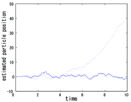
Figure 1: An example of the unstable autonomous trajectory (dot line) and the controlled stable trajectory (solid line) shown by $\pi_{t}(\hat{q})$.

Second, we describe the uncertainty included in the system. In particular, we consider two situations in which uncertain Hamiltonians $\Delta\hat{H}_{1}=-\sqrt{d_{t}}\hat{q}^{2}$ and $\Delta\hat{H}_{2}=\sqrt{d_{t}}\hat{q}^{2}$ are added to $\hat{H}_{1}$ and $\hat{H}_{2}$, respectively. The unknown time-varying parameter $d_{t}$ is bounded by the known constant $g\geq 0$, i.e., $d_{t}\in[0,g]$. Regarding the uncertainty in the system operator $\hat{c}$, on the other hand, we assume $\Delta\tilde{C}_{t}=0,~{}\forall t$. In this case, we can set $Q_{1}=\epsilon_{1}I,Q_{2}=(g/\epsilon_{1})I$, and $Q_{3}=0$ by choosing the parameters shown in the proof of Proposition 2.

The comparison of the three observers is performed based on the following evaluation. For the Kalman filter and the risk-sensitive observer, we evaluate the stationary mean square error between the “true” system and the estimator for the “nominal” system corresponding to $d_{t}=0$ (see Appendix C). In both cases, the tuning parameters in the cost function are set to Eq. (53). Next, for the robust observer, we evaluate the guaranteed upper bound of the estimation error ${\rm Tr}\hskip 1.9919ptP_{2}$ in Eq. (29). The control input in the robust observer is set to the stationary LQG controller for the nominal system: $u_{t}=Lx_{t}=-(2/r)B^{{\mathsf{T}}}K_{\infty}x_{t}$, where $K_{\infty}$ is the stationary solution of Eq. (II.1).

Let us now describe the simulation results. First, we consider the case in which the total system Hamiltonian is given by $\hat{H}=\hat{H}_{1}^{{\rm free}}+\hat{H}^{{\rm control}}+\Delta\hat{H}_{1}$. Table I lists the three estimation errors mentioned above for several values of $g$. Here, the uncertainty $d_{t}$ is set to the “worst case” $d_{t}=g$ for each value of $g$. In the first row of the table, the notation “N/A” indicates that the solution of the Lyapunov equation (98) does not satisfy $\bar{W}+{\rm i}\hbar\bar{\Sigma}/2\geq 0$. This implies that the error dynamics between the uncertain actual system and the nominal Kalman filter is unstable. In other words, the Kalman filter fails in the estimation. It should be noted that two excessively large values of the estimation error, which appear in the first and second rows, indicate that the error dynamics is nearly unstable. Therefore, it can be concluded that the Kalman filter and the risk-sensitive observer for the nominal system do not work well when the uncertainty $d_{t}~{}(=g)$ assumes a large. On the other hand, as shown in the third row in Table I, the robust observer is not very sensitive to the magnitude of the uncertainty and provides a good estimation even when $g$ is large. The above discussion suggests that the robust observer is possibly the best option for dealing with a large uncertainty. In other cases, the risk-sensitive observer should be used.

Next, we consider the second example, in which the total system Hamiltonian is given by the harmonic oscillator $\hat{H}=\hat{H}_{2}^{{\rm free}}+\hat{H}^{{\rm control}}+\Delta\hat{H}_{2}$. In this case, it is immediately observed in Table II that the estimation errors of the robust observer are always greater than those of the others, while the risk-sensitive observer shows a good performance, particularly when $g$ assumes a large value. Hence, in this case the risk-sensitive observer is the most appropriate.

An interesting feature of the robust observer is that in the case of both the harmonic and anti-harmonic Hamiltonians, it provides almost the same trend in the estimation errors with respect to $g$, whereas the Kalman filter and the risk-sensitive observer produce drastically different trends in the errors. This indicates that the structure of the robust observer is designed such that the estimation error is insensitive to the stability property of the system. However, this design policy sometimes leads to the over conservative stability of the error dynamics, and the estimation performance eventually reduces.

Table 1: Comparison of the Kalman, risk-sensitive, and robust observers, denoted by “KAL”, “RSK”, and “ROB”, respectively. The free Hamiltonian of the system is approximated by the anti-harmonic oscillator. In order to calculate the guaranteed upper bound of the estimation error of the robust observer, ${\rm Tr}\hskip 1.9919ptP_{2}$, parameters $\delta_{1}$ and $\delta_{2}$ are fixed to $0.1$, and $\epsilon_{1}$ is selected such that ${\rm Tr}\hskip 1.9919ptP_{2}$ takes the minimum value. The risk-sensitive parameter is $\mu=0.3$, and the Planck constant is set to unity: $\hbar=1$. Note that both the robust observer and the risk-sensitive observer are not identical to the Kalman filter even when $g=0$, because the parameters $\delta_{2}$ and $\mu$ are now set to non-zero values.

$g$	0.00	0.20	0.38	0.60	0.80	0.97
KAL	1.43	2.38	40.88	N/A	N/A	N/A
RSK	1.48	1.82	2.21	3.19	6.07	61.27
ROB	1.73	3.32	4.74	7.04	10.12	14.13

Table 2: Comparison of the three types of estimators in the case of the harmonic oscillator Hamiltonian. All parameters of the estimators are set to the same values in Table I.

$g$	0.00	0.20	0.40	0.60	0.80	1.00
KAL	1.40	1.37	1.40	1.44	1.47	1.50
RSK	1.44	1.38	1.38	1.39	1.40	1.41
ROB	1.68	3.23	4.79	6.84	9.80	14.48

V Conclusion

In this paper, we have considered a linear quantum system subjected to time-varying norm-bounded parametric uncertainties and developed a quantum version of the robust observer. Although in the linear case much of classical control theory can be applied to quantum systems, due to the unitarity of quantum evolution, the quantum uncertain system must have a specific structure with respect to the uncertainties, and its classical correspondence has not been studied; the resulting quantum robust observer has thus no classical analogue. The observer differs from both the optimal Kalman filter and the risk-sensitive observer; however, it guarantees the upper bound of the variance of the estimation error. We then investigated the robustness property of the three estimators mentioned above by considering a typical quantum control problem—feedback cooling of particle motion. This examination clarified that the robust observer is superior to the others when the autonomous system is unstable and is subjected to an unknown perturbation with a large magnitude. Therefore, we can conclude that the robust filtering method originally developed for classical systems is actually very effective for quantum systems as well. This fact implies that several robust control techniques in classical control theory (e.g., doyle ) will be applicable to uncertain quantum systems.

Appendix A Proof of Eqs. (50) and (51)

At first, we derive a simple yet useful matrix inequality. For any real matrices $X$ and $Y$, we obviously have

$$\Big{(}\sqrt{\epsilon}X-\frac{1}{\sqrt{\epsilon}}Y\Big{)}^{{\mathsf{T}}}\Big{(}\sqrt{\epsilon}X-\frac{1}{\sqrt{\epsilon}}Y\Big{)}\geq O,$$

where $\epsilon>0$ is a free parameter. The above inequality immediately leads to

$$X^{{\mathsf{T}}}Y+Y^{{\mathsf{T}}}X\leq\epsilon X^{{\mathsf{T}}}X+\frac{1}{\epsilon}Y^{{\mathsf{T}}}Y.$$ (54)

Next, let us define

$$\tilde{C}_{1}={\rm Re}\tilde{C},~{}~{}\tilde{C}_{2}={\rm Im}\tilde{C},~{}~{}\Delta\tilde{C}_{1}={\rm Re}\Delta\tilde{C},~{}~{}\Delta\tilde{C}_{2}={\rm Im}\Delta\tilde{C}.$$

(In this appendix, we omit the suffix $t$ for simplicity.) Then, the conditions (III) are represented by $\Delta\tilde{C}_{i}^{{\mathsf{T}}}\Delta\tilde{C}_{i}\leq r_{i}I~{}(i=1,2)$. Note that they lead to the scalar inequalities: $\Delta\tilde{C}_{i}\Delta\tilde{C}_{i}^{{\mathsf{T}}}\leq r_{i}~{}(i=1,2)$.

Now we are at the point to prove. Let us first derive the inequality (50). By a straightforward calculation, we obtain

$$\Delta\bar{A}=\bar{\Sigma}\Delta G\bar{E}+\bar{\Theta}_{1}\Delta\bar{J}_{1}\bar{E}+\bar{\Sigma}\Delta\bar{J}_{2}\bar{\Theta}_{2}$$

$$\hskip 30.00005pt\mbox{}+\bar{\Sigma}\Delta\tilde{C}_{1}^{{\mathsf{T}}}\Delta\tilde{C}_{2}\bar{E}-\bar{\Sigma}\Delta\tilde{C}_{2}^{{\mathsf{T}}}\Delta\tilde{C}_{1}\bar{E},$$

where $\bar{\Sigma}=-[\Sigma~{}\Sigma]^{{\mathsf{T}}}\in{\mathbb{R}}^{4\times 2},~{}\bar{E}=[I~{}O]\in{\mathbb{R}}^{2\times 4}$ and

$$\bar{\Theta}_{1}=\left[\begin{array}[]{cc}\Sigma\tilde{C}_{1}^{{\mathsf{T}}}&-\Sigma\tilde{C}_{2}^{{\mathsf{T}}}\\ \Sigma\tilde{C}_{1}^{{\mathsf{T}}}&-\Sigma\tilde{C}_{2}^{{\mathsf{T}}}-2k\\ \end{array}\right],~{}~{}\bar{\Theta}_{2}=\left[\begin{array}[]{cc}\tilde{C}_{2}&0^{{\mathsf{T}}}\\ -\tilde{C}_{1}&0^{{\mathsf{T}}}\\ \end{array}\right],$$ (59)

$$\Delta\bar{J}_{1}=\left[\begin{array}[]{c}\Delta\tilde{C}_{2}\\ \Delta\tilde{C}_{1}\\ \end{array}\right],~{}~{}\Delta\bar{J}_{2}=[\Delta\tilde{C}_{1}^{{\mathsf{T}}}~{}~{}\Delta\tilde{C}_{2}^{{\mathsf{T}}}].$$ (62)

We here denoted $0^{{\mathsf{T}}}=[0~{}0]$. Accordingly, the matrix $\Delta\bar{A}\bar{X}+\bar{X}\Delta\bar{A}^{{\mathsf{T}}}$ is now represented by

$$\Delta\bar{A}\bar{X}+\bar{X}\Delta\bar{A}^{{\mathsf{T}}}$$

$$=(\bar{\Sigma}\Delta G\bar{E})\bar{X}+\bar{X}(\bar{\Sigma}\Delta G\bar{E})^{{\mathsf{T}}}$$

$$\mbox{}+(\bar{\Theta}_{1}\Delta\bar{J}_{1}\bar{E})\bar{X}+\bar{X}(\bar{\Theta}_{1}\Delta\bar{J}_{1}\bar{E})^{{\mathsf{T}}}$$

$$\mbox{}+(\bar{\Sigma}\Delta\bar{J}_{2}\bar{\Theta}_{2})\bar{X}+\bar{X}(\bar{\Sigma}\Delta\bar{J}_{2}\bar{\Theta}_{2})^{{\mathsf{T}}}$$

$$\mbox{}+(\bar{\Sigma}\Delta\tilde{C}_{1}^{{\mathsf{T}}}\Delta\tilde{C}_{2}\bar{E})\bar{X}+\bar{X}(\bar{\Sigma}\Delta\tilde{C}_{1}^{{\mathsf{T}}}\Delta\tilde{C}_{2}\bar{E})^{{\mathsf{T}}}$$

$$\mbox{}-(\bar{\Sigma}\Delta\tilde{C}_{2}^{{\mathsf{T}}}\Delta\tilde{C}_{1}\bar{E})\bar{X}-\bar{X}(\bar{\Sigma}\Delta\tilde{C}_{2}^{{\mathsf{T}}}\Delta\tilde{C}_{1}\bar{E})^{{\mathsf{T}}}.$$ (63)

We are then able to apply Eq. (54) to evaluate bounds of each line in the above equation. For example, the second line has the following bound:

$$(\bar{\Sigma}\Delta G\bar{E})\bar{X}+\bar{X}(\bar{\Sigma}\Delta G\bar{E})^{{\mathsf{T}}}\leq\epsilon_{1}\bar{X}\bar{E}^{{\mathsf{T}}}\bar{E}\bar{X}+\frac{1}{\epsilon_{1}}\bar{\Sigma}\Delta G^{2}\bar{\Sigma}^{{\mathsf{T}}}$$

$$\hskip 107.00012pt\leq\epsilon_{1}\bar{X}\bar{E}^{{\mathsf{T}}}\bar{E}\bar{X}+\frac{g}{\epsilon_{1}}\bar{\Sigma}\bar{\Sigma}^{{\mathsf{T}}},$$

where here the assumption on the uncertainty (21) was used. The free parameter $\epsilon_{1}>0$ should be tuned appropriately. Next, for evaluating the third line of Eq. (A), we remark the following:

$$\Delta\bar{J}_{1}\Delta\bar{J}_{1}^{{\mathsf{T}}}\leq{\rm diag}\{2r_{2},~{}2r_{1}\}.$$ (64)

This inequality is easily seen; the relations $\Delta\tilde{C}_{i}\Delta\tilde{C}_{i}^{{\mathsf{T}}}\leq r_{i}~{}(i=1,2)$ lead to

$${\rm det}\Big{[}{\rm diag}\{2r_{2},~{}2r_{1}\}-\Delta\bar{J}_{1}\Delta\bar{J}_{1}^{{\mathsf{T}}}\Big{]}$$

$$\hskip 10.00002pt=\|\Delta\tilde{C}_{1}\|^{2}\|\Delta\tilde{C}_{2}\|^{2}-\langle{\Delta\tilde{C}_{1},\Delta\tilde{C}_{2}}\rangle\geq 0.$$

Here, $\|\bullet\|^{2}$ and $\langle{\bullet,\bullet}\rangle$ denote the standard Euclidean norm and inner product, respectively. By using Eqs. (54) and (64), we then obtain the following inequality:

$$(\bar{\Theta}_{1}\Delta\bar{J}_{1}\bar{E})\bar{X}+\bar{X}(\bar{\Theta}_{1}\Delta\bar{J}_{1}\bar{E})^{{\mathsf{T}}}$$

$$\hskip 10.00002pt\leq\epsilon_{2}\bar{X}\bar{E}^{{\mathsf{T}}}\bar{E}\bar{X}+\frac{1}{\epsilon_{2}}\bar{\Theta}_{1}\Delta\bar{J}_{1}\Delta\bar{J}_{1}^{{\mathsf{T}}}\bar{\Theta}_{1}^{{\mathsf{T}}}$$

$$\hskip 10.00002pt\leq\epsilon_{2}\bar{X}\bar{E}^{{\mathsf{T}}}\bar{E}\bar{X}+\frac{2}{\epsilon_{2}}\bar{\Theta}_{1}{\rm diag}\{r_{2},~{}r_{1}\}\bar{\Theta}_{1}^{{\mathsf{T}}}.$$

For the other lines of Eq. (A), we can use the same manner to have their bounds that do not depend on the uncertainties. As a result, we obtain the objective inequality $\Delta\bar{A}\bar{X}+\bar{X}\Delta\bar{A}^{{\mathsf{T}}}\leq\bar{X}\bar{Q}_{1}\bar{X}+\bar{Q}_{2}$, where

$$\bar{Q}_{1}:=\left[\begin{array}[]{cc}Q_{1}&O\\ O&O\\ \end{array}\right],$$ (67)

$$\bar{Q}_{2}:=\left[\begin{array}[]{cc}Q_{2}&Q_{2}\\ Q_{2}&Q_{2}\\ \end{array}\right]-\frac{4r_{1}}{\epsilon_{2}}\left[\begin{array}[]{cc}O&mk^{{\mathsf{T}}}\\ km^{{\mathsf{T}}}&km^{{\mathsf{T}}}+mk^{{\mathsf{T}}}-2kk^{{\mathsf{T}}}\\ \end{array}\right].$$ (72)

The matrices $Q_{1}$ and $Q_{2}$ are defined as follows.

$$Q_{1}:=(\epsilon_{1}+\epsilon_{2}+\epsilon_{4}+\epsilon_{5})I+\epsilon_{3}(\tilde{C}_{1}^{{\mathsf{T}}}\tilde{C}_{1}+\tilde{C}_{2}^{{\mathsf{T}}}\tilde{C}_{2}),$$ (73)

$$Q_{2}:=\Big{(}\frac{g}{\epsilon_{1}}+\frac{r_{1}+r_{2}}{\epsilon_{3}}+\frac{r_{1}r_{2}}{\epsilon_{4}}+\frac{r_{1}r_{2}}{\epsilon_{5}}\Big{)}I$$

$$\hskip 30.00005pt\mbox{}+\frac{2}{\epsilon_{2}}\Sigma(r_{2}\tilde{C}_{1}^{{\mathsf{T}}}\tilde{C}_{1}+r_{1}\tilde{C}_{2}^{{\mathsf{T}}}\tilde{C}_{2})\Sigma^{{\mathsf{T}}}.$$ (74)

The parameters $\epsilon_{i}>0~{}(i=1,\ldots,5)$ should be chosen appropriately.

Let us next derive Eq. (51). Similar to the previous case, we use Eq. (54) to obtain a bound that does not depend on the uncertainty. First, we immediately obtain

$$\Delta D=\hbar\Sigma\Big{[}\tilde{C}_{1}^{{\mathsf{T}}}\Delta\tilde{C}_{1}+\Delta\tilde{C}_{1}^{{\mathsf{T}}}\tilde{C}_{1}+\tilde{C}_{2}^{{\mathsf{T}}}\Delta\tilde{C}_{2}+\Delta\tilde{C}_{2}^{{\mathsf{T}}}\tilde{C}_{2}$$

$$\hskip 50.00008pt\mbox{}+\Delta\tilde{C}_{1}^{{\mathsf{T}}}\Delta\tilde{C}_{1}+\Delta\tilde{C}_{2}^{{\mathsf{T}}}\Delta\tilde{C}_{2}\Big{]}\Sigma^{{\mathsf{T}}}$$

$$\hskip 8.99994pt\leq\hbar\Sigma\Big{[}\epsilon_{6}\tilde{C}_{1}^{{\mathsf{T}}}\tilde{C}_{1}+\frac{r_{1}}{\epsilon_{6}}I+\epsilon_{7}\tilde{C}_{2}^{{\mathsf{T}}}\tilde{C}_{2}+\frac{r_{2}}{\epsilon_{7}}I$$

$$\hskip 50.00008pt\mbox{}+(r_{1}+r_{2})I\Big{]}\Sigma^{{\mathsf{T}}}=:Q_{3}^{\prime},$$

where $\epsilon_{6}>0$ and $\epsilon_{7}>0$ are free parameters. This readily leads to

$$\left[\begin{array}[]{cc}\Delta D&\Delta D\\ \Delta D&\Delta D\\ \end{array}\right]\leq\left[\begin{array}[]{cc}Q_{3}^{\prime}&Q_{3}^{\prime}\\ Q_{3}^{\prime}&Q_{3}^{\prime}\\ \end{array}\right].$$

Also, setting $X=[0^{{\mathsf{T}}}~{}k^{{\mathsf{T}}}]$ and $Y=[-\Delta m^{{\mathsf{T}}}~{}-\Delta m^{{\mathsf{T}}}]$ in Eq. (54), we obtain the following inequality:

$$-\hbar\left[\begin{array}[]{cc}O&\Delta mk^{{\mathsf{T}}}\\ k\Delta m^{{\mathsf{T}}}&k\Delta m^{{\mathsf{T}}}+\Delta mk^{{\mathsf{T}}}\\ \end{array}\right]$$ (77)

$$\hskip 10.00002pt\leq\hbar\left[\begin{array}[]{cc}\Delta m\Delta m^{{\mathsf{T}}}/\epsilon_{8}&\Delta m\Delta m^{{\mathsf{T}}}/\epsilon_{8}\\ \Delta m\Delta m^{{\mathsf{T}}}/\epsilon_{8}&\Delta m\Delta m^{{\mathsf{T}}}/\epsilon_{8}+\epsilon_{8}kk^{{\mathsf{T}}}\\ \end{array}\right]$$ (80)

$$\hskip 10.00002pt\leq\hbar\left[\begin{array}[]{cc}r_{2}I/\epsilon_{8}&r_{2}I/\epsilon_{8}\\ r_{2}I/\epsilon_{8}&r_{2}I/\epsilon_{8}+\epsilon_{8}kk^{{\mathsf{T}}}\\ \end{array}\right],$$ (83)

where $\epsilon_{8}>0$. Consequently, $\Delta\bar{D}$ is bounded by $\Delta\bar{D}\leq\bar{Q}_{3}$, where

$$\bar{Q}_{3}:=\left[\begin{array}[]{cc}Q_{3}&Q_{3}\\ Q_{3}&Q_{3}\\ \end{array}\right]+\hbar\epsilon_{8}\left[\begin{array}[]{cc}O&O\\ O&kk^{{\mathsf{T}}}\\ \end{array}\right],$$

and

$$Q_{3}:=\hbar\Big{(}\frac{r_{1}}{\epsilon_{6}}+\frac{r_{2}}{\epsilon_{7}}+\frac{r_{2}}{\epsilon_{8}}+r_{1}+r_{2}\Big{)}I$$ (84)

$$\hskip 30.00005pt\mbox{}+\hbar\Sigma(\epsilon_{6}\tilde{C}_{1}^{{\mathsf{T}}}\tilde{C}_{1}+\epsilon_{7}\tilde{C}_{2}^{{\mathsf{T}}}\tilde{C}_{2})\Sigma^{{\mathsf{T}}}.$$

Appendix B Upper bound lemma

We consider a matrix-valued differential equation of the form

$$\dot{P}_{t}=AP_{t}+P_{t}A^{{\mathsf{T}}}+BB^{{\mathsf{T}}}.$$ (85)

Lemma.  Suppose there exists a positive definite matrix $X>0$ such that the inequality $AX+XA^{{\mathsf{T}}}+BB^{{\mathsf{T}}}<0$ holds. Then, Eq. (85) has a unique stationary solution that satisfies

$$\lim_{t\rightarrow\infty}P_{t}\leq X.$$

Proof.  We readily see that the matrix $A$ is strictly stable; any eigenvalue of $A$ has a negative real part. Now, let us define $\delta P_{t}:=X-P_{t}$. Then, by using the assumption we have

$$\dot{\delta P}_{t}=-(AX+XA^{{\mathsf{T}}}+BB^{{\mathsf{T}}})+A\delta P_{t}+\delta P_{t}A^{{\mathsf{T}}}$$

$$\hskip 8.99994pt\geq A\delta P_{t}+\delta P_{t}A^{{\mathsf{T}}},$$

which yields $\delta P_{t}\geq{\rm e}^{At}\delta P_{0}{\rm e}^{A^{{\mathsf{T}}}t}$. We then obtain $\lim_{t\rightarrow\infty}\delta P_{t}\geq 0$ since $A$ is strictly stable. This shows the assertion. $~{}\blacksquare$

Appendix C Nominal-true systems difference

The objective here is to characterize the stationary mean square error between the “true” system (III) and the risk-sensitive observer (II.2) specifically designed for the “nominal” system (6). For this purpose, we calculate the symmetrized covariance matrix of the error vector $\hat{e}_{t}:=\hat{x}_{t}-\pi^{\mu}_{t}(\hat{x})$, where $\hat{x}_{t}$ and $\pi^{\mu}_{t}(\hat{x})$ are generated from Eqs. (III) and (II.2), respectively. Particularly, we now focus on the stationary observer. Thus, let us assume that the two Riccati equations (II.2) and (II.2) have unique steady solutions $V^{\mu}_{\infty}$ and $K^{\mu}_{\infty}$, respectively. Then, defining

$$b_{o}:=\frac{1}{\hbar}V^{\mu}_{\infty}F^{{\mathsf{T}}}+\Sigma^{{\mathsf{T}}}({\rm Im}\tilde{C})^{{\mathsf{T}}},~{}~{}L_{o}:=-\frac{2}{r}B^{{\mathsf{T}}}K^{\mu}_{\infty},$$

the stationary risk-sensitive observer is described by

$$d\pi^{\mu}_{t}(\hat{x})=(A+\mu V^{\mu}_{\infty}M+BL_{o})\pi^{\mu}_{t}(\hat{x})dt$$

$$\hskip 40.00006pt\mbox{}+b_{o}(dY_{t}-F\pi^{\mu}_{t}(\hat{x})dt).$$

We then see that the augmented vector $\bar{\zeta}_{t}=[\hat{x}_{t}~{}\hat{e}_{t}]^{{\mathsf{T}}}$ satisfies $d\bar{\zeta}_{t}=\bar{A}_{o}\bar{\zeta}_{t}dt+\bar{b}_{o}d\hat{B}_{t}+\bar{b}_{o}^{*}d\hat{B}_{t}^{\dagger}$, where

$$\bar{A}_{o}=\left[\begin{array}[]{cc}A+\Delta A+BL_{o}&-BL_{o}\\ \Delta A-\mu V^{\mu}_{\infty}M&A+\mu V^{\mu}_{\infty}M-b_{o}F\\ \end{array}\right],$$ (88)

$$\bar{b}_{o}=\left[\begin{array}[]{c}{\rm i}\Sigma\tilde{C}^{{\mathsf{T}}}\\ {\rm i}\Sigma\tilde{C}^{{\mathsf{T}}}-b_{o}\\ \end{array}\right].$$ (91)

Let $\bar{V}_{t}$ be the symmetrized covariance matrix of $\bar{\zeta}_{t}$. As mentioned in the proof of Theorem 1, this matrix satisfies $\langle{\bar{\zeta}_{t}\bar{\zeta}_{t}^{{\mathsf{T}}}}\rangle=\bar{V}_{t}+{\rm i}\hbar\bar{\Sigma}/2$. By using this relation, we obtain $d\bar{V}_{t}/dt=\bar{A}_{o}\bar{V}_{t}+\bar{V}_{t}\bar{A}_{o}^{{\mathsf{T}}}+\bar{D}_{o}$, where $\bar{D}_{o}$ is given by

$$\bar{D}_{o}=\left[\begin{array}[]{cc}D&D\\ D&D\\ \end{array}\right]$$ (94)

$$-\hbar\left[\begin{array}[]{c|c}O&[b_{o}{\rm Im}(\tilde{C})\Sigma]^{{\mathsf{T}}}\\ \hline\cr b_{o}{\rm Im}(\tilde{C})\Sigma&b_{o}{\rm Im}(\tilde{C})\Sigma+[b_{o}{\rm Im}(\tilde{C})\Sigma]^{{\mathsf{T}}}-b_{o}b_{o}^{{\mathsf{T}}}\\ \end{array}\right].$$ (97)

As a result, the variance of the estimation error is given by $\lim_{t\rightarrow\infty}\langle{\hat{e}_{t}^{\mathsf{T}}\hat{e}_{t}}\rangle=\bar{W}_{33}+\bar{W}_{44}$, where $\bar{W}$ is the stationary solution of the following Lyapunov equation:

$$\bar{A}_{o}\bar{W}+\bar{W}\bar{A}_{o}^{{\mathsf{T}}}+\bar{D}_{o}=O.$$ (98)

The estimation error between the true system and the Kalman filter designed for the nominal system is immediately evaluated by setting $\mu=0$ in the above discussion.

References

• (1) V. P. Belavkin, J. Multivariate Anal., 42, 171 (1992).
• (2) V. P. Belavkin, Commun. Math. Phys., 146, 611 (1992).
• (3) V. P. Belavkin, Theory Probab. Appl., 38, 573 (1993).
• (4) L. Bouten, M. Guta and H. Maassen, J. Phys. A, 37, 3189 (2004).
• (5) L. Bouten, R. van Handel, and M. R. James, arXiv:math.OC/0601741 (2006).
• (6) H. M. Wiseman, Phys. Rev. A, 49, 2133 (1994).
• (7) A. C. Doherty and K. Jacobs, Phys. Rev. A, 60, 2700 (1999).
• (8) L. K. Thomsen, S. Mancini and H. M. Wiseman, J. Phys. B, 35, 4937 (2002).
• (9) J. M. Geremia, J. K. Stockton and H. Mabuchi, Science, 304, 270 (2004).
• (10) R. van Handel, J. K. Stockton and H. Mabuchi, IEEE Trans. Automat. Contr., 50, 768 (2005).
• (11) H. M. Wiseman, A. C. Doherty, Phys. Rev. Lett., 94, 070405 (2005).
• (12) H. Mabuchi, Phys. Rev. A, 58, 123 (1998).
• (13) J. M. Geremia, J. K. Stockton, A. C. Doherty, and H. Mabuchi, Phys. Rev. Lett., 91, 250801 (2003)
• (14) J. K. Stockton, J. M. Geremia, A. C. Doherty, and H. Mabuchi, Phys. Rev. A, 69, 032109 (2004).
• (15) C. Ahn, A. C. Doherty and A. J. Landahl, Phys. Rev. A, 65, 042301 (2002).
• (16) C. Ahn, H. M. Wiseman, and G. J. Milburn, Phys. Rev. A, 67, 052310 (2003).
• (17) R. L. Hudson and K. R. Parthasarathy, Commun. Math. Phys., 93, 301 (1984).
• (18) D. H. Jacobson, IEEE Trans. Automat. Contr., 18, 2, 124 (1973).
• (19) A. Bensoussan and J. H. van Schuppen, SIAM J. Control Optim., 23, 599 (1985).
• (20) P. Dupuis, M. R. James, and I. R. Petersen, Math. Control, Systems and Signals, 13, 318 (2000).
• (21) I. R. Petersen and D. C. McFarlane, IEEE Trans. Automat. Contr., 39, 9, 1971 (1994).
• (22) L. Xie and Y. C. Soh, Syst. Contr. Lett., 1, 22, 123 (1994).
• (23) U. Shaked and C. E. de Souza, IEEE Trans. Signal Processing, 43, 11, 2474 (1995).
• (24) I. R. Petersen and A. V. Savkin, Robust Kalman filtering for signals and systems with large uncertainties, (Birkhauser, Boston, MA, 1999).
• (25) M. R. James, J. Opt. B: Quantum Semiclass. Opt. 7, 198 (2005).
• (26) M. R. James, Phys. Rev. A, 69, 032108 (2004).
• (27) L. Bouten and R. van Handel, arXiv:math-ph/0511021 (2005).
• (28) A. C. Doherty, S. Habib, K. Jacobs, H. Mabuchi, and S. M. Tan, Phys. Rev. A, 62, 012105 (2000).
• (29) K. Zhou and J. C. Doyle, Essentials of Robust Control, (Prentice-Hall, Inc., New Jersey, 1997).